
Identifying IP Address Types
As you learned in Chapter 6, “Numbering Systems,” IP addresses are 32 bits in length when expressed in binary. When humans work with IP addresses, however, it is usually done in what is called dotted decimal format. An IP address in this format looks like the following:
192.168.5.3
This format is called dotted decimal because the sections, or fields, are divided by dots, and the values are expressed in decimal instead of binary. Each of the four fields is called an octet because each section can be expressed in binary format by using 8 bits. So to convert 192.168.5.3 to its binary format, each decimal number would be converted to its equivalent in binary. Because each section is 8 bits in length, the result would be a string of 32 0s or 1s. The conversion of 192.168.5.3 is as follows:
There is more to understand about an IP address than its two formats, however. To understand how IP addresses are used to accomplish segmentation (or subnetting), you must understand the two parts of the IP address and their relationship to a second value that any device with an IP address will possess (which is the subnet mask). This section presents those concepts and introduces a set of IP addresses that have been specifically reserved for use on LANs.
Defining IP Address Classes
When IPv4 addressing was first designed, the IP addresses were organized into what are called classes. Five classes of addresses were defined, and the value of the first octet (the octet to the far left) determines the class in which an IP address resides. The standard defines this in binary terms. Three of the classes are intended for application to individual devices, one class is reserved for multicasting, and the fifth is labeled experimental.
When expressed in decimal format, the ranges of possible values for the first octet of the five classes are as follows:
Class A—1 to 126
Class B—128 to 191
Class C—192 to 223
Class D—224 to 239
Class E—240 to 255
The standard defines these classes in terms of the first octet in binary. It defines the bits at the far-left side of the first octet, which are called the most significant or the high-order bits. All IP addresses in the same class will share the values of these defined bits. For example, every IP address in Class C will have the most significant bits in the first octet set to 11.
The entire 127.0.0.0/8 network is missing from this list (reserved) because these addresses are used for diagnostics. This is discussed further later in this section.
HIGH-ORDER BITS
High-order bits, also referred to as the most significant bits, are the far-left bits in a bit pattern. They are termed most significant or high order because they are worth the most because of their position. For example, in the 8-bit pattern 11000000, the two leftmost bits are worth 128 and 64, respectively, which is higher than the value of any other bits in the pattern.
When expressed in this form, the five classes are as follows:
Class A—0000
Class B–1000
Class C—1100
Class D—1110
Class E—1111
Because the first three classes (A, B, and C) are used for individual devices, that is where our focus will be. These three classes, from the first address to the last address in the class, are as follows:
Class A—1.0.0.1–126.255.255.255
Class B—128.0.0.1–192.255.255.255
Class C—193.0.0.1–223.255.255.255
You may have noticed that some numbers are missing. The entire networks from 0.0.0.0–0.255.255.255 and 127.0.0.0–127.255.255.255 are not used. The first is called the zero network and is arbitrarily not used, and the second (127.0.0.0–127.255.255.255) is reserved for network diagnostics. Any of the IP addresses in the 127.0.0.0 network can be used to test a computer. If the address can be pinged successfully, the computer has the TCP/IP protocol installed and the network adaptor card is functioning.
The most famous of the IP addresses in the 127.0.0.0 network (127.0.0.1) is called the local host. It is also known as the loopback address, as it loops the signal back through the network card for an answer if you ping it. Although any of the IP addresses in the 127.0.0.0 networks will do this, 127.0.0.1 gets all the glory.
You will learn how to use the loopback address to troubleshoot in the section “Utilizing Diagnostic Tools” later in this chapter.
Identifying Network and Host Addresses
Each IP address has two parts, the network part and the host part. These two portions function in a manner similar to your street address and your house number. The network portion determines the LAN in which the computer is located, and the host portion identifies the computer in that LAN. The network portion begins at the far-left side of the IP address and continues uninterrupted until it meets the host portion. The host portion then continues to the far-right side of the IP address.
The point in the address at which the network portion ends and the host portion begins is determined by the class of the IP address. The computer uses a second value called the subnet mask to determine which portion is network and which portion is host. When the computer reads the subnet mask, each octet that is 255 is considered to be network, and each octet that is 0 is considered to be host. It then uses the octets that are set to the value of 255 to mask the network portion (which means it uses the mask to determine the network part). A computer cannot have an IP address without also having a subnet mask. The addressing is incomplete if both values are not present.
In classful IP addressing, the dividing line between the two is always done between octets. An example of an IP address from each class with the network part shaded red and host part shaded green is shown in Figure 7.2. Figure 7.2 also shows the subnet mask for each class. As you can see, the parts of the subnet mask that are 255s match the network portion of the address.
Classful IP addressing is the IP addressing system used from 1981 until 1993. It creates only three classes of networks for unicast communication. Chapter 8 discusses the limitations this imposes.

FIGURE 7.2 Subnet masks for each class
In the next chapter, it will be important for you to be comfortable working with subnet masks in binary form, so let's take a look at what the three default subnet masks look like:
Class A (255.0.0.0)
11111111.00000000.00000000.00000000
Class B (255.255.0.0)
11111111.11111111.00000000.00000000
Class C (255.255.255.0)
11111111.11111111.11111111.00000000
DEFAULT SUBNET MASKS
A default subnet mask is one that conforms to the rules of classful subnetting. In Chapter 8, you will learn that other subnet mask possibilities exist and are used to create networks of the size desired. As you will learn, this removes the restriction of only having three sizes of networks to choose from in design.
As you already know, the computer evaluates everything in binary, so when the computer reads the subnet mask, 1s indicate the network portion and 0s indicate the host portion. It is also important to know that the string of 1s indicating the network portion is never interrupted by 0s, which means there will never be a subnet mask like this:
11100011.00000000.00000000.00000000
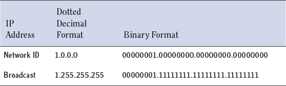
In each network or LAN, there are two IP addresses that can never be assigned to devices. These addresses are reserved for special roles in each network. The first is called the network ID and second is called the broadcast address. These two addresses can be identified in the LAN by the bits in the host portion of the IP address. If all of the bits in the host portion are 0s, then the address is the network ID. If all of the bits in the host portion are 1s (or 255s in decimal), the address is called the broadcast address. An example of a Class A network ID and broadcast address in both binary and dotted decimal form is shown here:
The network ID is used to identify the network as a group. It is an important value that routers use in the routing tables. If this value were not available to identify the entire LAN, a router would have to have an entry for every host, which would make the routing tables huge and would slow the routing process to a crawl. By using this value, the router can route packets to any computer in a LAN, and then the router that physically connects to that LAN will locate the specific host at the Network Access layer by using the ARP broadcast method you learned about in Chapter 3.
The broadcast address is used any time a computer needs to send a packet to every host in its LAN. An example of a broadcast is an ARP broadcast. Hosts broadcast in other instances as well. Later in this chapter, you will learn about the operation of Dynamic Host Configuration protocol (DHCP). When DHCP is used, the computers broadcast to locate the DHCP server.
The number of possible networks per class is a function of the possible combinations of the number of bits dedicated to the network portion for the class. For example, if 2 bits were used for the network (which is not possible in classful IP addressing, because 8 bits is the minimum, but consider this example just for illustration purposes) the possible combinations using 2 bits would be as follows:
00
01
10
11
Those are the only combinations using 2 bits. Because there are four possible combinations using 2 bits, it would mean you could have four networks, each identified by the values in the first 2 bits. To determine the number of possible networks given the number of bits dedicated to the network portion of the address, the following formula can be used:
2n = number of possible networks
where n = the number of bits in the network portion
To prove this formula manually, we can use the previous 2-bit example. Because 22 = 4, the formula works. That means that for a Class A network in which 8 bits (the entire first octet) are used for the network portion, the number of networks possible would be 28, which is 256. Using this formula and applying it to each of the three classes of networks, the number of possible networks for each is shown here:
| Network Class | Number of Possible Networks |
| Class A | 28 = 256 |
| Class B | 216 = 65,536 |
| Class C | 224 = 16,777,216 |
Just as the number of bits dedicated to the network portion of the address determines the number of possible Class A, B, and C networks, the number of host bits determines the possible number of computers in a Class A, B, and C network. The number of computers possible in each class network is a function of the number of possible combinations of numbers using the number of host bits. The formula for the number of possible computers in a network is
Using a Class C address as an example (which has 8 host bits, which is the entire last octet), the possible number of computers would be as follows:
28 – 2 = 254
Can you guess why we are subtracting 2 from the possible number of computers in each network? Remember the two IP addresses that are reserved in each network (network ID and broadcast). We must subtract those out to get the number of available IP addresses in each network. Using this formula and applying it to each of the three classes of networks, the number of possible computers for each is shown here:
| Network Class | Number of Possible Computers |
| Class A | 224 - 2 = 16,777,214 |
| Class B | 216 - 2 = 65,534 |
| Class C | 28 - 2 = 254 |
Because there are only three classes in classful IP addressing, there are only three sizes of networks. In the next chapter, you will learn the limitations that restriction introduces and how classless IP addressing solves those problems.
Describing Private IP Addresses and NAT
When IPv4 was created, it was thought that the number of possible IP addresses would be sufficient to serve the Internet. However, after a few years of incredible growth, it became apparent that this was not the case. The eventual solution was IPv6, which you will learn about later in this chapter. While the IPv6 system was still in development, two temporary solutions were implemented to delay the eventual exhaustion of the address space. These two solutions were classless IP addressing (which you will learn about in the next chapter) and private IP addressing used in conjunction with Network Address Translation (NAT) services.
Up until the time that private IP addressing and NAT services were introduced, all computers that were to connect to the Internet had to have a unique IP address issued from the entities managing the Internet. Therefore, a company with 500 computers that required Internet access would be issued a block of 500 unique addresses from their Internet service provider. Then the NAT server was introduced, which allowed a single server to be the gateway to the Internet for the entire company, to represent all 500 computers on the Internet with a single IP address.
When Network Address Translation is in use, the computers in the network have IP addresses that need not be unique on the Internet. When one of these computers needs to go to the Internet, their packet will go to the NAT server. The NAT server will remove the IP address of the computer and replace it with the IP address of the NAT server. Therefore, when the packet is sent to the web server on the Internet, the source IP address will be that of the NAT server. When the page is returned from the web server to the NAT server, the NAT server will forward the page back to the computer, using the IP address of the computer as the destination.
If you understand how Network Address Translation works, it really doesn't matter what IP addresses you use in your LAN as long as they are unique within the LAN. Because these IP addresses are never seen on the Internet (because they get translated to a public address that is unique on the Internet), you could use any addresses you like.
Having said that, three special ranges of IP addresses have been reserved for use inside LANs. The IP addresses in these ranges are called private IP addresses. These ranges were specified in Request for Comments (RFC) 1918.
There is a range in each address class. These addresses are not given out for use on the Internet. There is no requirement to use them in a LAN, but it has become a common practice to do so.
Before a standard is adopted and published, it is presented to the standards body in a document called a Request for Comments (RFC).
These ranges are as follows:
Class A—10.0.0.0 to 10.255.255.255
Class B—172.16.0.0 to 172.31.255.255
Class C—192.168.0.0 to 192.168.255.255