Chapter 15

Phasing in Phasors for Wave Functions

In This Chapter

Describing circuit behavior with phasors

Mixing phasors with impedance and Ohm’s law

Applying phasor techniques to circuits

Phasors — not to be confused with the phasers from Star Trek — are rotating vectors you can use to describe the behavior of circuits that include capacitors and inductors. Phasors make the analysis of such circuits easier because instead of dealing with differential equations, you just have to work with complex numbers. I don’t know about you, but I’d take working with complex numbers to solve circuits any day over using differential equations.

Phasor analysis applies when your input is a sine wave (or sinusoidal signal). A phasor contains information about the amplitude and phase of the sinusoidal signal. Frequency isn’t part of phasor form because the frequency doesn’t change in a linear circuit.

This chapter introduces phasors and explains how they represent a circuit’s i-v characteristics. I then show you how phasors let you summarize the complex interactions among resistors, capacitors, and inductors as a tidy value called impedance. Finally, you see how phasors let you analyze circuits with storage devices algebraically, in the same way you analyze circuits with only resistors.

Taking a More Imaginative Turn with Phasors

A phasor is a complex number in polar form. When you plot the amplitude and phase shift of a sinusoid in a complex plane, you form a phase vector, or phasor.

As I’m sure you’re well aware from algebra class, a complex number consists of a real part and an imaginary part. For circuit analysis, think of the real part as tying in with resistors that get rid of energy as heat and the imaginary part as relating to stored energy, like the kind found in inductors and capacitors.

You can also think of a phasor as a rotating vector. Unlike a vector having magnitude and direction, a phasor has magnitude VA and angular displacement ϕ. You measure angular displacement in the counterclockwise direction from the positive x-axis.

Figure 15-1 shows a diagram of a voltage phasor as a rotating vector at some frequency, with its tail at the origin. If you need to add or subtract phasors, you can convert the vector into its x-component (VA cos ϕ) and its y-component (VA sin ϕ) with some trigonometry.

Illustration by Wiley, Composition Services Graphics

Figure 15-1: A phasor is a rotating vector in the complex plane.

The following sections explain how to find the different forms of phasors and introduce you to the properties of phasors.

Finding phasor forms

Phasors, which you describe with complex numbers, embody the amplitude and phase of a sinusoidal voltage or current. The phase is the angular shift of the sinusoid, which corresponds to a time shift t0. So if you have cos[ω(t – t0)], then ωt0 = ϕO, where ϕO is the angular phase shift.

To establish a connection between complex numbers and sine and cosine waves, you need the complex exponential ejθ and Euler’s formula:

where .

The left side of Euler’s formula is the polar phasor form, and the right side is the rectangular phasor form. You can write the cosine and sine as follows:

Re[ ] denotes the real part of a complex number, and Im[ ] denotes the imaginary part of a complex number.

Figure 15-2 shows a cosine function and a shifted cosine function with a phase shift of π/2. In general, for the sinusoids in Figure 15-2, you have an amplitude VA, a radian frequency ω, and a phase shift of ϕ given by the following expression:

Because the radian frequency ω remains the same in a linear circuit, a phasor just needs the amplitude VA and the phase ϕ to get into polar form:

To describe a phasor, you need only the amplitude and phase shift (not the radian frequency). Using Euler’s formula, the rectangular form of the phasor is

Illustration by Wiley, Composition Services Graphics

Figure 15-2: Cosine functions.

Examining the properties of phasors

One key phasor property is the additive property. If you add sinusoids that have the same frequency, then the resulting phasor is simply the vector sum of the phasors — just like adding vectors:

For this equation to work, phasors V1, V2, …, VN must have the same frequency. You find this property useful when using Kirchhoff’s laws.

Another vital phasor property is the time derivative. The time derivative of a sine wave is another scaled sine wave with the same frequency. Taking the derivative of phasors is an algebraic multiplication of jω in the phasor domain. First, you relate the phasor of the original sine wave to the phasor of the derivative:

But the derivative of a complex exponential is another exponential multiplied by jω:

Based on the phasor definition, the quantity (jωV) is the phasor of the time derivative of a sine wave phasor V. Rewrite the phasor jωV as

When taking the derivative, you multiply the amplitude VA by ω and shift the phase angle by 90°, or equivalently, you multiply the original sine wave by jω. See how the imaginary number j rotates a phasor by 90°?

Working with capacitors and inductors involves derivatives because things change over time. For capacitors, how quickly a capacitor voltage changes directs the capacitor current. For inductors, how quickly an inductor current changes controls the inductor voltage.

Using Impedance to Expand Ohm’s Law to Capacitors and Inductors

The concept of impedance is very similar to resistance. You use the concept of impedance to formulate Ohm’s law in phasor form so you can apply and extend the law to capacitors and inductors. After describing impedance, you use phasor diagrams to show the phase difference between voltage and current. These diagrams show how the phase relationship between the voltage and current differs for resistors, capacitors, and inductors.

Understanding impedance

For a circuit with only resistors, Ohm’s law says that voltage equals current times resistance, or V = IR. But when you add storage devices to the circuit, the i-v relationship is a little more, well, complex. Resistors get rid of energy as heat, while capacitors and inductors store energy. Capacitors resist changes in voltage, while inductors resist changes in current. Impedance provides a direct relationship between voltage and current for resistors, capacitors, and inductors when you’re analyzing circuits with phasor voltages or currents.

Like resistance, you can think of impedance as a proportionality constant that relates the phasor voltage V and the phasor current I in an electrical device. Put in terms of Ohm’s law, you can relate V, I, and impedance Z as follows:

The impedance Z is a complex number:

Here’s what the real and imaginary parts of Z mean:

The real part R is the resistance from the resistors. You never get back the energy lost when current flows through the resistor. When you have a resistor connected in series with a capacitor, the initial capacitor voltage gradually decreases to 0 if no battery is connected to the circuit. Why? Because the resistor uses up the capacitor’s initial stored energy as heat when current flows through the circuit. Similarly, resistors cause the inductor’s initial current to gradually decay to 0.

The imaginary part X is the reactance, which comes from the effects of capacitors or inductors. Whenever you see an imaginary number for impedance, it deals with storage devices. If the imaginary part of the impedance is negative, then the imaginary piece of the impedance is dominated by capacitors. If it’s positive, the impedance is dominated by inductors.

When you have capacitors and inductors, the impedance changes with frequency. This is a big deal! Why? You can design circuits to accept or reject specific ranges of frequencies for various applications. When capacitors or inductors are used in this context, the circuits are called filters. You can use these filters for things like setting up fancy Christmas displays with multicolored lights flashing and dancing to the music.

The reciprocal of impedance Z is called the admittance Y:

The real part G is called the conductance, and the imaginary part B is called susceptance.

Looking at phasor diagrams

Phasor diagrams explain the differences among resistors, capacitors, and inductors, where the voltage and current are either in phase or out of phase by 90°. A resistor’s voltage and current are in phase because an instantaneous change in current corresponds to an instantaneous change in voltage. But for capacitors, voltage doesn’t change instantaneously, so even if the current changes instantaneously, the voltage will lag the current. For inductors, current doesn’t change instantaneously, so when there’s an instantaneous change in voltage, the current lags behind the voltage.

Figure 15-3 shows the phasor diagrams for these three devices. For a resistor, the current and voltage are in phase because the phasor description of a resistor is VR = IRR. The capacitor voltage lags the current by 90° due to –j/(ωC), and the inductor voltage leads the current by 90° due to jωL.

Illustration by Wiley, Composition Services Graphics

Figure 15-3: Phasor diagram of a resistor, capacitor, and inductor.

Putting Ohm’s law for capacitors in phasor form

For a capacitor with capacitance C, you have the following current:

Because the derivative of a phasor simply multiplies the phasor by jω, the phasor description for a capacitor is

The phasor description for a capacitor has a form similar to Ohm’s law, showing that a capacitor’s impedance is

Figure 15-3 shows the phasor diagram of a capacitor. The capacitor voltage lags the current by 90°, as you can see from Euler’s formula:

Think of the imaginary number j as an operator that rotates a vector by 90° in the counterclockwise direction. A –j rotates a vector in the clockwise direction. You should also note j2 rotates the phasor by 180° and is equal to –1.

The imaginary component for a capacitor is negative. As the radian frequency ω increases, the capacitor’s impedance goes down. Because the frequency for a battery is 0 and a battery has constant voltage, the impedance for a capacitor is infinite. The capacitor acts like an open circuit for a constant voltage source.

Putting Ohm’s law for inductors in phasor form

For an inductor with inductance L, the voltage is

The corresponding phasor description for an inductor is

The impedance for an inductor is

Figure 15-3 shows the phasor diagram of an inductor. The inductor voltage leads the current by 90° because of Euler’s formula:

The imaginary component is positive for inductors. As the radian frequency ω increases, the inductor’s impedance goes up. Because the radian frequency for a battery is 0 and a battery has constant voltage, the impedance is 0. The inductor acts like a short circuit for a constant voltage source.

Tackling Circuits with Phasors

Phasors are great for solving steady-state responses (assuming zero initial conditions and sinusoidal inputs). Under the phasor concept, everything I cover in earlier chapters can be reapplied here. You can take functions of voltages v(t) and currents i(t) described in time to the phasor domain as V and I. With phasor methods, you can algebraically analyze circuits that have inductors and capacitors, similar to how you analyze resistor-only circuits.

When analyzing circuits in the phasor domain for sine or cosine wave (sinus-oidal signal) inputs, use these steps:

1. Transform the circuit into the phasor domain by putting the sinusoidal inputs and outputs in phasor form.

2. Transform the resistors, capacitors, and inductors into their impedances in phasor form.

3. Use algebraic techniques to do circuit analysis to solve for unknown phasor responses.

4. Transform the phasor responses back into their time-domain sinusoids to get the response waveform.

Using divider techniques in phasor form

In a series circuit with resistors, capacitors, inductors, and a voltage source, you can use phasor techniques to obtain the voltage across any device in the circuit. You can generalize the series circuit and voltage divider concept in Chapter 4 by replacing the resistors, inductors, and capacitors with impedances.

Remember that in a series circuit, you have the same current flowing through each device. When a series circuit is driven by a voltage source, you can find the voltage across each device using voltage divider techniques. This involves multiplying a voltage source by the ratio of the desired device impedance to the total impedance of the series circuit.

The top diagram of Figure 15-4 shows an RLC (resistor, inductor, capacitor) series circuit to illustrate the voltage divider concept and series equivalence:

You have an equivalent impedance ZEQ from the three devices:

Here’s the equivalent impedance for the RLC series circuit in Figure 15-4:

Illustration by Wiley, Composition Services Graphics

Figure 15-4: Voltage and current divider techniques in the phasor domain.

To get the voltage V3 = VC, use the voltage divider technique:

Now plug in the values for Z3 and ZEQ to get the capacitor voltage (V3 = VC):

You can also obtain the equivalent impedance for parallel circuits and use the current divider method. (To see how to derive the equivalent resistance and current divider equations, see Chapter 4.) Parallel devices have the same voltage, which helps you get the total admittance (the reciprocal of impedance Z):

For the RLC parallel circuit in Figure 15-4, the equivalent admittance is

To find the capacitor current I3 = IC, use the current divider technique:

Plugging in the values for Y1 and YEQ, the capacitor current I3 = IC is

Adding phasor outputs with superposition

Superposition (see Chapter 7) says you can find the phasor output due to one source by turning off other sources; you then get the total output by adding up the individual phasor outputs.

You can use the superposition technique in phasor analysis only if all the independent sources have the same frequency. Superposition doesn’t work when you have different frequencies in the independent sources — you treat each source separately to get its steady-state output contribution to the total output.

To see how superposition works with phasors, first look at the top circuit in Figure 15-5. The middle diagram turns off VS2, leaving VS1 as the only voltage source. Use the voltage divider method to get the capacitor voltage VC1 due to VS1:

where // denotes the parallel connection of capacitor C and resistor R.

The parallel combination of R and C has an equivalent impedance of

Illustration by Wiley, Composition Services Graphics

Figure 15-5: Super-position in the phasor domain.

The bottom diagram of Figure 15-5 turns off VS1, leaving only VS2 turned on. You use the voltage divider technique with capacitor C and inductor L connected in parallel to get the capacitor voltage due to VS2:

The parallel combination of L and C has an equivalence impedance:

The total output voltage is the sum of VC1 and VC2 due to each source:

Simplifying phasor analysis with Thévenin and Norton

You can use the Thévenin and Norton equivalents — which I first discuss in Chapter 8 with resistive circuits — in the phasor domain as well. The Thévenin equivalent simplifies a complex array of impedances and independent sources to one voltage source connected in series with one impedance value (a complex number in general). The Norton equivalent simplifies a complex array of impedances and independent sources to one current source connected in parallel with one impedance value. The two equivalents are related by a source transformation. You use the Thévenin and Norton equivalents when you’re analyzing different loads to a source circuit.

The Thévenin and Norton equivalents in Figure 15-6 follow the same approach as the one you’d use for resistive circuits. You simply calculate the open-circuit phasor voltage VOC and short-circuit phasor current ISC for each equivalent circuit.

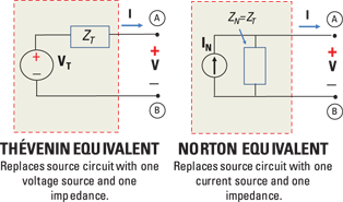
Illustration by Wiley, Composition Services Graphics

Figure 15-6: Thévenin and Norton equivalents in phasor domain.

The following phasor equations are similar to corresponding equations for resistive circuits:

Using VOC and ISC, you find Thévenin impedance ZT as follows:

Alternatively, you can calculate the impedance ZT by looking back to the source circuit between Terminals A and B with all independent sources turned off, as described in Chapter 8.

Figure 15-7 shows a circuit to illustrate the Thévenin equivalent between Terminals A and B. Because you have an open-circuit load, no current flows through resistor R. You can find the open-circuit voltage using the voltage divider technique:

Illustration by Wiley, Composition Services Graphics

Figure 15-7: Example of the Thévenin equivalent in the phasor domain.

Putting a short across Terminals A and B implies that the resistor R and capacitor C are connected in parallel. The current flowing through this combination is

The short-circuit current ISC flows through R. Using the current divider technique, you get

You find the impedance ZT by taking the ratio of VOC/ISC:

Getting the nod for nodal analysis

When the circuit is large and complex, node-voltage analysis allows you to reduce the number of equations you need to deal with simultaneously. From the smaller set of node voltages, you can find any voltage or current for any device in the circuit. The node-voltage analysis technique I describe in Chapter 5 also works in the algebraic phasor domain. Figure 15-8 shows an op-amp circuit where you can use node-voltage analysis techniques. (For the scoop on op amps, see Chapter 10.)

Illustration by Wiley, Composition Services Graphics

Figure 15-8: Op-amp node analysis in phasor form.

At Node A, you have the following KCL equation:

For ideal op amps with negative feedback, you have the inverting current IN = 0 and VN = VP = 0. Solve for the output VO in terms of the input VS:

The output is an inverted input multiplied by the ratio of impedances. If the input impedance Z1 is due to a resistor and feedback impedance Z2 is due to a capacitor, then the phasor output VO is

This equation should look familiar, because it’s the integrator of the function waveform vS(t). You see that the 1/jω term describes the phasor for an integrator. That’s how an integrator is done electronically with op amps — beautiful!

Using mesh-current analysis with phasors

Mesh-current analysis is useful when a circuit has several loops. From the smaller set of mesh currents, you can find any voltage or current for any device in the circuit.

You can open up the mesh analysis approach in Chapter 6 to the phasor domain. You simply replace each device with its phasor impedance and apply KVL for each mesh to develop the mesh current equations. Figure 15-9 helps show the phasor analysis of circuits using mesh current techniques.

Illustration by Wiley, Composition Services Graphics

Figure 15-9: Mesh-current analysis using phasors.

The circuit has two mesh currents, IA and IB, and five devices. For Meshes A and B, KVL produces the following:

Replace the phasor voltages with the corresponding mesh currents and impedances:

You then collect like terms and rearrange the mesh current equations to put them in standard form:

Convert the equations to matrix form:

Note the symmetry along the diagonal of the first matrix. For circuits with independent sources, this symmetry is a useful check to verify that your mesh current equations are correct.

You can then use matrix software to solve for the unknown mesh currents IA and IB, which you use to find the device currents and voltages.