
Chapter 11. Personalized Recommendation Metrics
Having explored the powerful methodologies of Matrix Factorization and Neural Networks in the context of personalization, we are now equipped with potent tools to craft sophisticated recommendation systems. However, the order of recommendations in a list may have a profound impact on user engagement and satisfaction.
Our journey so far has primarily been focused on predicting what a user may like, using latent factors or deep learning architectures. However, the manner in which we present these predictions, or more formally, how we rank these recommendations, holds paramount significance. Therefore, this chapter will shift our gaze from the prediction problem, and will unravel the complex landscape of ranking in recommendation systems.
This chapter is dedicated to understanding key ranking metrics including: Mean Average Precision (MAP), Mean Reciprocal Rank (MRR), and Normalized Discounted Cumulative Gain (NDCG). Each of these metrics takes a unique approach towards quantifying the quality of our rankings, catering to different aspects of the user interaction.
We’ll dive into the intricacies of these metrics, unveiling their computational details and discussing their interpretation, covering their strengths and weaknesses, and pointing out their specific relevance to different personalization scenarios.
This exploration forms an integral part of the evaluation process in recommendation systems. It not only gives us a robust framework to measure the performance of our system but also provides essential insights into understanding how different algorithms might perform in online settings. This will lay the foundation for future discussions on algorithmic bias, diversity in recommendations, and a multi-stakeholder approach to recommendation systems.
In essence, the knowledge garnered in this chapter will be instrumental in fine-tuning our recommendation system, ensuring that we don’t just predict well, but also recommend in a way that truly resonates with individual user preferences and behaviors.
Environments
Before we dig into defining the key metrics, we’re going to spend a few moments discussing the kinds of evaluation one can do. Evaluation for recommendation systems – as you’ll soon see – are frequently characterized by how “relevant” the recommendation are for a user. This is very similar to search metrics, but we add in additional factors to account for where in the list the most relevant items are.
For an extremely comprehensive view on evaluation of recommender systems, the recent project RecList builds a useful checklist-based framework for organizing metrics and evaluations.
Often you’ll hear about evaluating recommenders in a few different setups:
-
online/offline
-
user/item
-
A/B
Each of these are slightly different kinds of evaluations, and tell you different things. Let’s quickly break down the differences to set some assumptions about terminology
Online and Offline
When we refer to online vs. offline recommenders we are referring to when you’re running evals. Offline evaluation is when you start with a test/evaluation dataset, outside your production system, and compute a set of metrics. This is often the simplest to set up, but has the highest expectation of existing data. Using historical data, you construct a set of relevant responses, which you can then use during simulated inference. This is the most similar to other kinds of traditional Machine Learning, although with slightly different computations for the error.
When we’re training large models, these datasets are very similar to an offline dataset. We previously saw prequential data, which is much more relevant in Recommendation Systems than in lots of other ML applications. Sometimes you’ll hear people say that “all recommenders are sequential recommenders” because of how important historical exposure is to the recommender problem.
Online evaluation takes place during inference, usually in prod. The tricky part is, you essentially never know the counter-factual outcomes. You can compute specific metrics on the online rankings: frequency and distributions of covariates, click-through-rate/success-rate, or time-on-platform, but ultimately these are different than the offline metrics.
Bootstrapping from historical evaluation data
One of the most common questions from people building a recommender from scratch is “where do you get the initial training data”? This is a hard problem. Ultimately, one has to be clever to come up with a useful dataset. Consider our co-occurrence data in the Wikipedia recommender – that didn’t require any user interactions to get to a set of data to build a recommender. Bootstrapping from item-to-item is the most popular strategy, but there are some other tricks as well. The simplest way to start moving into user-item recommenders, is to simply ask the user questions. If you ask the user to provide preference information across a set of item features, you can build simple models which start to incorporate this.
User vs. Item metrics
Because Recommender Systems are personalization machines, it can be very easy to think that we always want to be making recommendations for the user, and measuring the performance as such. There are some subtleties, though. We want to be sure individual items are getting a fair chance, and sometimes looking at the other side of the equation can help us assess this. In other words, are the items getting recommended frequently enough to have a chance to find their niche. We should explicitly compute our metrics over user and item axes.
Another aspect of item-side metrics, is for set-based recommenders. The other items that are recommended in context, can have a very significant effect on the performance of a recommendation. As a result, we should be careful to measure the pairwise item metrics in our large scale evaluations.
A/B testing
It’s good to use randomized, controlled trials to evaluate if your new recommendation model is performing. For recommendations, this is quite tricky. We’ll see at the end of this chapter some of the nuance in this, but for now, let’s consider a quick reminder of how to think about A/B testing in a closed-loop paradigm.
A/B tests are ultimately attempting to estimate the effect size of swapping one model in for another – effect size estimation is the process of measuring the causal impact of an intervention on a target metric. First, we would need to deploy two recommender models. We’d also hope that there’s a reasonable randomization of users into each of the recommenders. However, what’s the randomization unit? It’s easy to quickly assume it’s the user, but what has changed about the recommender? Has the recommender changed in a way that covaries with some properties of the distribution, e.g. have you built a new recommender that is less friendly towards seasonal TV specials just as we enter into the second week of November?
Another consideration with this sort of testing for recommendation systems is the long term compounding effects. A frequent rejoinder about a series of positive A/B test outcomes over several years is “have you tested the first recommender against the last?”. This is because populations change, both the users and the items. As you vary also the recommender system, you frequently find yourself in a double-blind situation where you’ve never seen this user or item population with any other recommender. If all the effect-sizes of every A/B test was additive across the industry, the world GDP would likely be 2-3 times as large.
The way to guard against protests like this is via something called a long-term holdout, i.e. a set of random subset (continually being added to) users who will not be upgraded to new models through time. By measuring the target metrics on this set vs. the most cutting edge model in production, you’re always able to understand the long term effects of your work. The downside of a long-term holdout? They’re hard to maintain, and it’s hard to sacrifice some of the effects of your work on a subset of the population.
Now let’s finally get to the metrics already!
Recall and Precision
Let’s begin by considering four recommender problems, and how each of them may have different implications for the kind of results you may want.
First, let’s consider entering a bookstore and looking for a book by a popular author. We would say this is the recommender problem:
-
provides a lot of recommendations
-
few possible relevant results
Additionally, if the bookstore has a good selection, we’d expect that all of the relevant results are contained in the recommendations because bookstores often carry most or all of an author’s ouvre once they’ve become popular. However, many of the recommendations – the books in the bookstore – are simply not relevant for this search.
Second, let’s consider looking for a gas station nearby on mapping app while in a large metro. We expect that there are a lot of gas stations relatively close by, but you would probably only consider the first couple – or maybe even only one; the first one that you see. Thus a recommender for this problem has:
-
many relevant results
-
few useful recommendations.
Those are two very simple scenarios when the relevant results may be fully contained in the recommendations, and when the recommendations may be fully contained in the relevant results respectively.
Let’s now look at more common scenarios.
Third, consider that you’re searching on a streaming video platform for something to watch tonight when you’re feeling romantic. Streaming platforms tend to show a lot of recommendations, pages and pages from this one theme or another. But on this night, and on just this platform, there may only be a couple movies or TV shows that really fit what you’re looking for. Our recommender then:
-
provides many recommendations
-
only a few things out there are actually relevant
However, importantly, not all relevant results will be in the recommendations! As we know, different platforms have different media, so some of the relevant results wont appear in the recommendations no matter how many we look at.
Fourth and finally, you’re a high-end coffee lover with distinguished taste headed into the local roaster for a 3rd wave single origin coffee. As an experienced coffee connoisseur, you love high quality coffees from all over the world, and enjoy most but not all origins. On any given day your local cafe only has a few single-origin hand brew options on bar. Despite your worldly palette, there are some popular terroirs that you just don’t love. This little recommendation brew bar:
-
provides a few recommendations
-
many possible recommendations are relevant
but on a given day, only some of the few recommendations may be relevant to you.
Here we have seen the four scenarios of matching. Note: for the latter two, the intersection between recommendation and relevant, may be proportionally small or large – or even empty! The main idea, is that the full size of the smaller sample is not always in use.
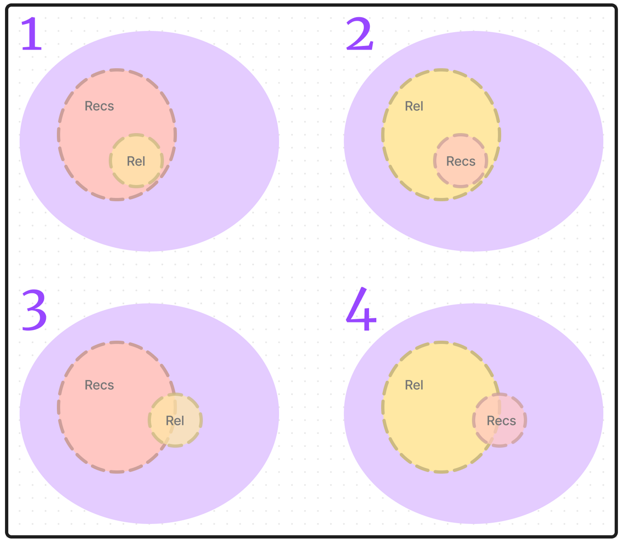
Figure 11-1. Recall and Precision sets
Now that we’ve worked through a few examples, let’s see how they relate to the core metrics for a recommender, precision and recall @ k. Focusing on examples 3 and 4, we can see that only some of the recs intersect with the options that are relevant. And only some of the relevants intersect with the recs. It’s often overlooked, but in fact these two ratios define our metrics – let’s go!
@ K
In much of this chapter and recsys metrics discussion, we say things like @ K. This means “at K” which should really be “in K” or “out of K”. These are simply the size of the set of recommendations. We will often anchor the customer experience on “how many recommendations we can show to the user without the experience suffering. We also will need to know the cardinality of the set of relevant items, which we call @ R. Note that while it may not feel like it’s possible to ever know this number, we assume this refers to “known relevant” via our training or test data.
Precision at K
Precision is the ratio of the size of the set relevant recommendations to K, the size of the set of recommendations.
Notice that the size of the relevant items doesn’t appear in the formula. That’s ok, the size of the intersection is still dependent on the size of the set of relevant items.
Looking at our examples, technically 2 has the highest precision, but it’s a bit of red herring because of how many relevant results there are. This is one reason why precision is not the most common metric for evaluating recommendation systems.
Recall at K
Recall is the ratio of the size of the set of relevant recommendations to R, the size of the set of relevant items.
But wait! If the ratio is the relevant recommendations over the relevant items, where is K? K is still important here because the size of the set of recommendations constrains the possible size of the intersection. Recall that these ratios are operating on that intersection which is always dependent on K. This means you often consider the max of R and K.
In scenario three, we hope that some of the movies that fit our heart’s desire will be on the right streaming platform. The number of these divided by the count of all the media anywhere is the recall. If all your relevant movies are on this platform, you might call that Total Recall.
Scenario four’s cafe experience shows that recall is sometimes the “inverse probability of an avoid”; because you like so many coffees we might instead find it easier to talk about what you don’t like. In this case, the number of avoids in their offering will have a large effect on the recall:
This is the core mathematical definition for recall, and is often one of the first measurements we’ll consider due to the fact that it’s a pure estimate of how your retrieval is performing.
R-precision
If we also have a ranking on our recommendations we can take the ratio of relevant recommendations to R in the top-R recommendations. This improves this metric in cases where R is very small – like examples one and three.
MAP, MMR, NDCG
Having delved into the reliable domains of Precision@k and Recall@k, we’ve gained valuable insights into the quality of our recommendation systems. However, these metrics, as crucial as they are, can sometimes fall short in capturing an important aspect of these systems - the order of recommendations.
In recommendation systems, the ordering in which we present suggestions carries significant weight and needs to be evaluated to ensure it’s effective.
That’s why we’ll now journey beyond Precision@k and Recall@k to explore some key ranking-sensitive metrics, namely Mean Average Precision (mAP), Mean Reciprocal Rank (MRR), and Normalized Discounted Cumulative Gain (NDCG). These metrics not only consider whether our recommendations are relevant, but also whether they are well-ordered.
MAP lends importance to each relevant document and its position, MRR concentrates on the rank of the first relevant item, and NDCG gives more importance to relevant documents at higher ranks. By understanding these metrics, you’ll have an even more robust set of tools to evaluate and refine your recommendation systems.
So, let’s carry on with our exploration, striking a balance between precision and comprehensibility. By the end of this section, you will be well-equipped to handle these essential evaluation methods in a confident and knowledgeable manner.
MAP
This is a vital metric in recommendation systems, and it’s particularly adept at accounting for the rank of relevant items. If, in a list of five items, the relevant ones are found at positions 2, 3, and 5, mAP would be calculated by computing precision@2, precision@3, and precision@5, and then taking an average of these values. The strength of mAP lies in its sensitivity to the ordering of relevant items, providing a higher score when these items are ranked higher.
Consider an example with two recommendation algorithms A and B:
-
For Algorithm A, we compute the mAP as: mAP = (precision@2 + precision@3 + precision@5) / 3 = (1/2 + 2/3 + 3/5) / 3 = 0.6
-
For Algorithm B, which perfectly ranks the items, mAP is calculated as: mAP = (precision@1 + precision@2 + precision@3) / 3 = (1/1 + 2/2 + 3/3) / 3 = 1
The generalized formula for mAP across a set of queries Q is:
Here,
MRR
Another effective metric used in recommendation systems is MRR. Unlike MAP, which considers all relevant items, MRR primarily focuses on the position of the first relevant item in the recommendation list. It’s computed as the reciprocal of the rank where the first relevant item appears.
Consequently, MRR can reach its maximum value of 1 if the first item in the list is relevant. If the first relevant item is found further down the list, MRR takes a value less than 1. For instance, if the first relevant item is positioned at rank 2, the MRR would be 1/2.
Let’s look at this in the context of the recommendation algorithms A and B that we used earlier:
-
For Algorithm A, the first relevant item is at rank 2, so the MRR equals 1/2 = 0.5.
-
For Algorithm B, which perfectly ranked the items, the first relevant item is at rank 1, so the MRR equals 1/1 = 1.
Extending this to multiple queries, the general formula for MRR is:
Here, |Q| represents the total number of queries and
NDCG
To further refine our understanding of ranking metrics, let’s step into the world of NDCG. Like mAP and MRR, NDCG also acknowledges the rank order of relevant items, but it introduces a twist. It discounts the relevance of items as we move down the list, signifying that items appearing earlier in the list are more valuable than those ranked lower.
NDCG begins with the concept of Cumulative Gain (CG), which is simply the sum of the relevance scores of the top k items in the list. Discounted Cumulative Gain (DCG) takes a step further, discounting the relevance of each item based on its position. NDCG, then, is the DCG value normalized by the Ideal DCG (IDCG), the DCG that we would obtain if all relevant items appeared at the very top of the list.
Assuming we have five items in our list and a specific user for whom the relevant items are found at positions 2 and 3, the IDCG@k would be (1/log(1 + 1) + 1/log(2 + 1)) = 1.5 + 0.63 = 2.13.
To put this into the context of our example algorithms A and B:
For Algorithm A:
-
DCG@5 = 1/log(2 + 1) + 1/log(3 + 1) + 1/log(5 + 1) = 0.63 + 0.5 + 0.39 = 1.52
-
NDCG@5 = DCG@5 / IDCG@5 = 1.52 / 2.13 = 0.71
For Algorithm B:
-
DCG@5 = 1/log(1 + 1) + 1/log(2 + 1) + 1/log(3 + 1) = 1 + 0.63 + 0.5 = 2.13
-
NDCG@5 = DCG@5 / IDCG@5 = 2.13 / 2.13 = 1
The general formula for NDCG can be represented as:
where
-
-
and
This metric gives us a normalized score for how well our recommendation algorithm ranks relevant items, discounting as we move further down the list.
MAP vs NDCG?
Both MAP and NDCG are holistic metrics that offer a comprehensive perspective of ranking quality by incorporating all relevant items and their respective ranks. However, the interpretability and use cases of these metrics can vary based on the specifics of the recommendation context and the nature of relevance.
While MRR does not consider all relevant items, it does provide an interpretable insight into an algorithm’s performance, highlighting the average rank of the first relevant item. This can be particularly useful in scenarios where the top-most recommendations hold significant value.
mAP, on the other hand, is a rich evaluation measure that effectively represents the area under the Precision-Recall curve. Its average aspect confers an intuitive interpretation related to the trade-off between precision and recall across different rank cutoffs.
NDCG introduces a robust consideration of the relevance of each item and is sensitive to the rank order, employing a logarithmic discount factor to quantify the diminishing significance of items as we move down the list. This allows it to handle scenarios where items can have varying degrees of relevance, extending beyond binary relevance often used in mAP and MRR. However, this versatility of NDCG can also limit its interpretability due to the complexity of the logarithmic discount.
Further, although NDCG is well-equipped for use cases where items carry distinct relevance weights, procuring accurate ground-truth relevance scores can pose a significant challenge in practical applications. This imposes a limitation on the real-world usefulness of NDCG.
Cumulatively, these metrics form the backbone of offline evaluation methodologies for recommendation algorithms. As we advance in our exploration, we’ll cover online evaluations, discuss strategies to assess and mitigate algorithmic bias, understand the importance of ensuring diversity in recommendations, and optimize recommendation systems to cater to various stakeholders in the ecosystem.
Correlation coefficients
While correlation coefficients like Pearson’s or Spearman’s can be employed to evaluate the similarity between two rankings (for instance, between the predicted and the ground truth rankings), they do not provide the exact same information as MAP, MRR, or NDCG.
Correlation coefficients are typically used to measure the degree of linear association between two continuous variables, and in the context of ranking, they can indicate the overall similarity between two ordered lists. However, they do not directly account for aspects such as the relevance of individual items, the position of relevant items, or varying degrees of relevance among items, which are integral to mAP, MRR, and NDCG.
For example, consider a scenario where a user has interacted with five items in the past. A recommender system might predict that the user will interact with these items again, but rank them in the opposite order of importance. Even though the system has correctly identified the items of interest, the reversed ranking would lead to poor performance as measured by mAP, MRR, or NDCG, but a high negative correlation coefficient would be obtained due to the linear relationship.
As a result, while correlation coefficients can provide a high-level understanding of ranking performance, they are not sufficient substitutes for the more detailed information provided by metrics like mAP, MRR, and NDCG.
To utilize correlation coefficients in the context of ranking, it would be essential to pair them with other metrics that account for the specific nuances of the recommendation problem, such as the relevance of individual items and their positions in the ranking.
RMSE from affinity
Root Mean Square Error (RMSE) and ranking metrics like MAP, MRR, and NDCG offer fundamentally different perspectives when evaluating a recommendation system that outputs affinity scores.
RMSE is a popular metric for quantifying prediction error. It computes the square root of the average of squared differences between the predicted affinity scores and the true values. Lower RMSE signifies better predictive accuracy. However, RMSE treats the problem as a standard regression task and disregards the inherent ranking structure in recommendation systems.
Conversely, mAP, MRR, and NDCG are explicitly designed to evaluate the quality of rankings, which is essential in a recommendation system. In essence, while RMSE measures the closeness of predicted affinity scores to actual values, mAP, MRR, and NDCG assess the ranking quality by considering the positions of relevant items. Therefore, if your main concern is ranking items rather than predicting precise affinity scores, these ranking metrics are generally more appropriate.
Integral forms: AUC and cAUC
When it comes to recommendation systems, we are producing a ranked list of items for each user. As we’ve seen these rankings are based on affinity, the probability or level of preference that the user has for each item. Given this framework, several metrics have been developed to evaluate the quality of these ranked lists. One such metric is the AUC-ROC, which is complemented by mAP, MRR, and NDCG. Let’s take a closer look at understanding these.
Recommendation Probabilities to AUC-ROC
In a binary classification setup, the Area Under the Receiver Operating Characteristic Curve (AUC-ROC) measures the ability of the recommendation model to distinguish between positive (relevant) and negative (irrelevant) instances. It is calculated by plotting the True Positive Rate (TPR) against the False Positive Rate (FPR) at various threshold settings, then computing the area under this curve.
In the context of recommendations, you can think of these “thresholds” as varying the number of top items recommended to a user. The AUC-ROC metric becomes an evaluation of how well your model ranks relevant items over irrelevant ones, irrespective of the actual rank position. In other words, AUC-ROC effectively quantifies the likelihood that a randomly chosen relevant item is ranked higher than a randomly chosen irrelevant one by the model. This, however, doesn’t account for the actual position or order of items in the list, only the relative ranking of positive versus negative instances. The affinity of an item when calibrated may be interpreted as a confidence measure by the model that an item is relevant, and when considering historical data, even uncalibrated affinity scores may make a great suggestion both for the number of recs necessary to find something useful.
One very serious implementation of these affinity scores might be to only show users items over a particular score; otherwise telling the user to come back later or utilizing some exploration methods to improve your data. For example if you sold hygeine products and were considering asking customers to add on some Aesop soap during checkout, you may wish to evaluate the Aesop ROC and only make this suggestion when the observed affinity passed the learned threashold. We’ll also see these concepts used later during our discussion of “Inventory Health”.
Comparison to Other Metrics
-
Mean Average Precision (mAP): this metric expands on the idea of precision at a specific cut-off in the ranked list to provide an overall measure of model performance. It does this by averaging the precision values computed at the ranks where each relevant item is found. Unlike AUC-ROC, mAP puts emphasis on the higher-ranked items and is more sensitive to changes at the top of the ranking.
-
Mean Reciprocal Rank (MRR): Unlike AUC-ROC and mAP which consider all relevant items in the list, MRR focuses only on the rank of the first relevant item in the list. It is a measure of how quickly the model can find a relevant item. If the model consistently places a relevant item at the top of the list, it will have a higher MRR.
-
Normalized Discounted Cumulative Gain (NDCG): this metric evaluates the quality of the ranking by not only considering the order of recommendations but also taking into account the graded relevance of items (which the previous metrics don’t). NDCG discounts items further down the list, rewarding relevant items that appear near the top of the list.
AUC-ROC provides a valuable aggregate measure of a model’s ability to differentiate between relevant and irrelevant items, mAP, MRR, and NDCG offer a more nuanced evaluation of the model’s ranking quality, considering factors like position bias and varying degrees of relevance.
Note that we sometimes compute the AUC on a per-customer basis and then average. That’s cAUC and can often provide a good expectation for a user’s experience.
BPR
Bayesian Personalized Ranking (BPR) presents a Bayesian approach to the task of item ranking in recommendation systems, effectively providing a probability framework to model the personalized ranking process. Instead of transforming the item recommendation problem into a binary classification problem (relevant or not), BPR focuses on pairwise preferences, i.e., given two items, which one does the user prefer? This approach aligns better with the nature of implicit feedback that is common in recommendation systems.
The BPR model uses a pairwise loss function that takes into account the relative order of a positive item and a negative item for a specific user. It seeks to maximize the posterior probability of the observed rankings being correct. The model is typically optimized using stochastic gradient descent or some variant thereof. It’s important to note that BPR, unlike other metrics we’ve discussed including AUC-ROC, mAP, MRR, and NDCG, is a model training objective rather than an evaluation metric. Therefore, while the aforementioned metrics evaluate a model’s performance post-training, BPR provides a mechanism to guide the model learning process in a way that directly optimizes for the ranking task. A much deeper discussion of these topics is in [Rendle et al](https://dl.acm.org/doi/10.5555/1795114.1795167).
Summary
Now that we know how to evaluate the performance of the recommendation systems that we train, you may be finding yourself wondering how we will actually train them. You may have noticed that many of the metrics we introduced would not make very good loss functions; they involve a lot of simultaneous observations about sets and lists of items. This would unfortunately make the signal that the recommender would be learning from highly combinatorial. Additionally, in the metrics we’ve seen there are really two aspects to consider: the binary metric associated to Recall, and the rank weighting.
In the next chapter, we’re going to learn some loss functions that make excellent training objectives. The importance of these, I’m sure wont be lost on you.