
Chapter 9. Feature based and counting-based recommendations
Consider the over-simplified problem: given a bunch of new users, predict which users will like our new mega-ultra-fancy-fun-item-of-novelty, or M.U.F.F.I.N. for short. You may start by asking which old users like MUFFIN; do those users have any aspects in common? If so you could build a model that predicts MUFFIN affinity from those correlated user features.
Alternatively, you could ask “what are some other items people buy with MUFFIN?”; if you find that others frequently also ask for JAM – Just-Awesome-Merch – then MUFFIN may be a good suggestion for those who already have JAM. This would be using the co-occurrence of MUFFIN and JAM as a predictor. Similarily, if your friend comes along with very similar taste to you – you both like SCONE, JAM, BISCUIT, and TEA – but he’s not yet had the MUFFIN, if you like MUFFIN it’s probably a good choice for him too. This is using the co-occurrence of items between you and your friend.
These will form our first ranking methods in this chapter; so grab a tasty snack and let’s dig in.
Bilinear factor models (metric learning)
As per the usual idioms about running in front of horses and walking after the cart, let’s start our journey into ranking systems with what can be considered the naive machine learning approaches. Via these approaches, we will start to get a sense of where the rub lies in building recommendation systems, and why some of the forthcoming efforts are necessary at all.
Let’s begin again with our basic premise of recommendation problems: to estimate ratings of item
Now, we consider user
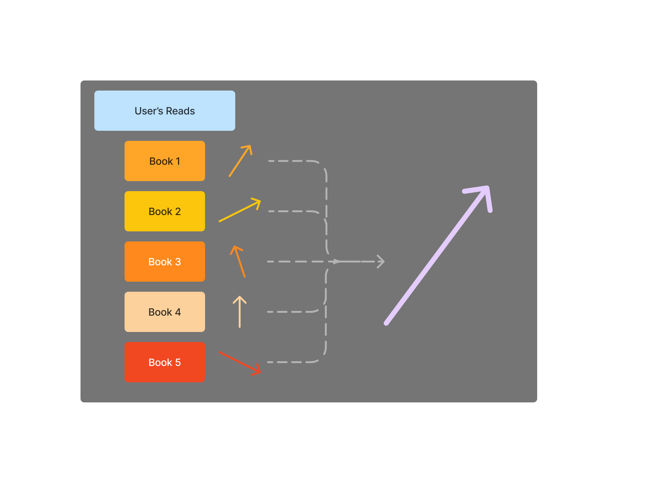
Figure 9-1. Content to feature vector
This extremely simple approach can turn a collection of item features and user-item interactions, into features of the user. Much of the following, will be more and more rich ways of doing this. Thinking very hard about the map, the features, and the requirements for interaction, yield many of the key insights in the rest of the book.
Let’s take the above mapping,
We need move back to the mathematical framings to set up how to use these vectors. Ultimately, we’re now in a latent space with users and items, but how can we do anything with that? Well you may already remember how to compare vector similarity. Let’s define the similarity to be cosine-similarity, so:
If we pre-compose our similarity with vector-normalization, this is simply the inner-product–and this, is an essential first step towards recommendation systems. For convenience, let’s always assume this space we’re working in is after normalization, so all similarity measures are done on the unit sphere;
now approximates our ratings. But wait, dear reader, where are the learnable parameters? Let’s go ahead and make this a weighted summation, via a diagonal matrix
This very slight generalization already puts us in the world of statistical learning. You can probably already see how
nets us even more parameters! We see that now
so:
If we make up notation for the right hand side, you’ll find your friend linear regression waiting for you:
thus:
With this computation behind us, we see that whether we wish to compute binary ratings, ordinal ratings, or likelihood estimation, the tools in our linear models toolbox can enter the party. We have available to us regularization and optimizers and any other fun we’re interested in from the linear models world.
If these equations feel frustrating or painful, let me try to offer you a geometric mental model. Each item and user is in a high dimensional space and ultimately we’re trying to figure out which ones are closest to one another. Where people frequently misunderstand these geometries is that they imagine the tips of the vectors being near one another – this is not the case. These spaces are extremely high-dimensional which results in the analogy being far from the truth. Instead, ask if the values are similarly large in some of the vector indices. This is a much more simple, but also more accurate geometric view: that there are some subspaces in the extremely high-dimensional space where the vectors point in the same direction.
This forms the foundation for where we are going however, this has serious limitations for large scale recommender problems. We will see, however, the feature based learning still has it’s place–in the cold-start regime.
Note that in addition to the above approach of building content-based features for a user, we may also have obvious user features that are obtained via queries to the user, or implicitly via other data collection; examples of these features include location, age-range, or height.
Is user space the same as item space?
Above we discuss ways to put users and items in the same latent spaces. We claim that we can make comparisons between users and items by vector operations. In mathematics, vectors are elements of vector spaces, and (finite dimensional) vector spaces are defined by their number of dimensions and the values that the vectors have as elements. For example, if we say it’s a 3-dimensional vector space with 8bit integers, that’s sufficient to specify a vector space. However, there are some devilish details lurking around. The first of which is what distance means in a specified vector space. We have many conventional measures, but it’s important to ensure comparisons between two spaces are utilizing the same definitions of distance. Another consideration is the process by which you define the vectors of the space; if you arrive at your vectors via a dimension reduction from a larger space, there are likely density properties that you can expect not present naively. Where this is most relevant for ranking models and recommendation systems is that we frequently arrive at user space and item space separately, and very often compute distance between user and item vectors.
Is this ok? In many cases, it lacks firm theoretical footing, but works well. One particular case where this does have a firm theoretical footing is Matrix Factorization. Rather than a long digression on Geometric Algebra, we will give the following guidance: if you’re interested comparing two vectors that aren’t in the same space, ask yourself if they’re of the same dimension, if distance is defined the same in both spaces, and if the density priors are similar. In fact, there are times where none of the above are true and you can still get away with a comparison. But for each of the above, it’s worth a stop-and-think. One very explicit example of a troubling difference in two latent spaces is found in this paper on hierarchical representations; the space that is learned in this paper is a very interesting way to encode relationships between items in your latent space via the implicit geometry. However, your users may not be encoded in a hyperbolic space–tread carefully if you compute inner products between these and euclidean embedded vectors!
Feature-based warm starting
As we saw in Chapter 7, there are a variety of approaches to using features along side some of the collaborative filtering and matrix factorization approaches we’ve seen. In particular, we saw how encoders build via a two-towers architecture can be used for fast feature-based recommendations in the cold-start scenario. Let’s look into this deeper, and think carefully about features for new users or items.
In the previous, we saw our bilinear factor model built as a simple regression, and in fact we saw that all the standard machine learning modeling approaches would apply. However, we took the user-embedding to be features learned from item-interactions: that is, the content-based feature vector. If our goal is to build a recommendation algorithm that does not need a history of user ratings, obviously this construction will not suffice.
We might begin by asking if the factor regression approach above could work in the pure user-feature setting–leave aside worries about the inner-product that depended on a mutual embedding, and just take everything to be pure matrices. While this is a reasonable idea that can yield some results, we may quickly identify the coarse-ness of this model: each user would then need to provide answers to queries
Because we intend on using collaborative filtering via matrix factorization as our core model, we’d really like to find a way to smoothly transition from the feature-based model, into this MF ensuring we take advantage of user/item ratings as they emerge. In our discussion of the Data Flywheel we discussed how inference results and their subsequent outcomes can be used in real time to update the model, but how do we account for that in the modeling paradigm?
In a latent-factor model obtained via matrix factorization, we have
where
More mathematically: we learn a regression model
where our
Note that this approach actually provides a very general strategy for including features into a matrix factorization model. How we fit the factors-features model is totally up to us, as are the optimization methods we wish to employ.
Also note that instead of regression based approaches, priors can be established via KNN in a purely feature-based embedding space. This modeling strategy is explored in great detail in the survey by Abdullah et. al. 2021. Compare this with the item-item content-based recommender from Chapter 5, where the query is an item, and similarity in item-space is the link between the last item and the next.
We have established a strategy and a collection of approaches to building our models via features. We’ve even seen how our matrix factorization will fall over for new users, only to be saved by a feature based model. So why not stick to features? Why introduce factors at all?
Segmentation models and hybrids
Similar to the above discussion of warm-starting via features, is the closely related concept of demographic-based systems. Note that demographic in this context need not refer explicitly to personally identifiable information, it can simple refer to the user data collected during the signup process. Some simple examples from book recommendations might include a user’s favorite genres, self-identified price preference, book-length preferences, favorite author, and so on. Standard methods of clustering-based regression, can be helpful in converting a small set of user features into recommendations for new users. For these coarse user features, building simple feature based models like naive-bayes, can be especially effective.
More generally, given user feature vectors, we can formulate a similarity measure and then user segments to make new-user recommendations. This should feel very similar to feature based recommenders, but instead, we do not require usage of user-features, we instead model the user’s containment in a segment, and then build our factor model from the segment to different items.
One way to imagine this approach is to consider the modeling problem as estimating:
for
While these ideas may not seem like interesting extensions to what we’ve build previously, in practice, they can be enormously useful for fast, explainable recommendations for new users.
Also note that nothing in this construction is particular to the users; we can consider the dual model which takes the clustering to be at the level of the items and performs a similar process. Combining these models can provide the most coarse model of simply user-segments to item-groups, and utilizing several of these modeling approaches simultaneously can provide important and flexible models.
Tag based recommenders
One special case of the segmentation model for item-based recommenders is a tag-based recommender. This is a quite common first recommender to try, when you have some human labels and need to quickly turn this into a working recommender. Let’s talk through a toy example: you have a personal digital wardrobe, where you’ve logged many features about each article of clothing in your personal closet. You want your fashion recommender to give you suggestions for what else to wear, given that you’ve selected one piece for the day. You wake up, and see that it’s rainy outside so you start by choosing a cozy cardigan. The model you’ve trained has found that cardigan has tags outerwear and cozy, which it knows correlate well with bottoms and warm–so it’s likely to recommend you some heavier jeans today.
The upside of a tag recommender, is how explainable and understandable the recommendations are. The downside, is that performance is directly tied to how much effort is put into tagging items.
Let’s discuss a slightly more involved example of a tag-based recommender that one of the Authors built – in collaboration with Ashraf Shaik and Eric Bunch – for recommending blog posts.
The goal was to warm-start the blog post recommender utilizing high-quality tags that classified the blogs into themes. One thing that was special about this tagging system, is that it was a very rich hierarchical tagging system maintained by the marketing team. In particular, each tag type had several different values, and there were 11 tag types with up to 10 values each. Blogs had values for each tag type, and sometimes had multiple tags in a single tag type for the blog. This may sound a bit complicated, but suffice to say each blog post could have some of the 47 tags, and the tags were further grouped into types.
One first thing that could be done, is to simply use those tags to build a simple recommender, and we did, but that would be missing a very important additional opportunity when afforded such high quality tag data – evaluating our embeddings.
First, we needed to understand how we could build user embeddings – our plan was to average the blog-embeddings a user had seen, a very simple collaborative filtering approach when you have a clear item-embedding. Thus we wanted to train the best embedding model possible for these blogs. We started by considering models like BERT, but we were unsure if the highly technical content would be meaningfully captured by our embedding model. This led us to realize that we could use the tags as a classifier dataset for our embedding – if we could test several different embedding models by training a simple MLP to perform multi-label multi-classification for each of the tag types, where the input features were the embedding dimensions, then our embedding space captured well the content. Some of the embedding models were of varying dimensions, and some were quite large, so we also first used a dimension reduction (UMAP) to a standard size before we trained the MLP. We used [F1 scores](https://scikit-learn.org/stable/modules/generated/sklearn.metrics.f1_score.html) to determine which of the embedding models led to the best classification model for tags, and did some visual inspection to ensure the groups were as we’d hoped. This worked quite well and showed that some embeddings were much better than others.
Hybridization
We saw in the previous section how we can blend our matrix factorization with simpler models via taking priors from the simpler models, and learning how to transition away. There are more coarse approaches to this process of hybridization.
-
As mentioned before; weighted combinations of models is incredibly powerful, and the weights can be learned in a standard bayesian framework.
-
multi-level modeling can include learning a model to select which recommendation model should be used, and then learning models in each regime–for example utilize a tree-based model on user features when the user has <10 historical ratings and then use MF after that. There are a variety of multi-level approaches including switching and cascading which correspond roughly to voting vs boosting.
-
feature augmentation which allows multiple vectors of features to be concatenated and a larger model be learned. By definition, if we wish to combine feature vectors with factor vectors, like those coming from a collaborative filter, we will expect substantial nullity. Learning despite that nullity allows a somewhat naive combination of the different kinds of features to be fed into the model and operated on in all regimes of user activity.
There are a variety of useful ways to combine these models, however we take the position that instead of more complicated combinations of several models that work well in different paradigms, we will attempt to stick to a relatively straightforward model-service architecture:
-
we will train the best model we can using matrix factorization based collaborative filtering
-
we will utilize user and item feature-based models for cold start.
Let’s see why we might think feature-based modeling may not be the best strategy, even if we do it via Neural Networks and latent factor models.
Limitations of Bilinear models
In the above, we started by describing bilinear modeling approaches, and immediately one should take warning–they’re linear relationships. We can immediately wonder: “are there really linear relationships between the features of my users and items and the pairwise affinity?”
The answer to this question might depend on the number of features, or it may not. Either way, skepticism is appropriate, and in practice the answer is overwhelmingly no. You might think “well then as it is a linear approximation, matrix factorization so too cannot succeed”, but that’s not so clear cut. In fact, matrix factorization suggests that the linear relationship is between the latent factors, not the actual features. This subtle difference makes a world of difference.
One important call-out before we move on to simpler ideas is that Neural Networks with non-linear activation functions can be used to build feature based methods. There are some successes in this domain, but ultimately a surprising and important result is that Neural Collaborative Filtering does not outperform Matrix Factorization. This doesn’t suggest that there are not useful approaches for feature based models utilizing MLP’s, but it does defray some of our worries about MF being too-linear. So why not more feature based approaches?
The first most obvious challenge for content-based, demographic-based, and any other feature-based method is getting the features. Let’s consider the dual problems:
-
features for users; if we want to collect features for users we need either ask them a series of queries, or infer those features implicitly. Inferring these via exogenous signals is noisy and limited, but each query that we ask the user increases the likelihood of onboarding drop-off. When we think of user-onboarding funnels we know that each additional prompt or question incurs another chance that the user will not complete the onboarding. This accumulates quickly and without users making it through the funnel, the recommendation system wont be very useful.
-
features for items; on the flip side, creating features for items is a heavily manual task. While many businesses need to do this task to serve other purposes also, it still incurs a significant cost in many cases. If the features are to be useful, they need to be of high quality, which incurs more debt. But most importantly, if the number of items is extremely large, the cost may quickly get out of reach. For large-scale recommendation problems, it is simply infeasible to manually add features. This is where automatic feature engineering models can help.
Another significant issue in these feature based models is separability or distinguishability. These models are not useful if the features cannot separate well the items or users. This leads to compounding problems as the cardinality increases.
Finally, in many recommendation problems, we start with the assumption that taste or preference is extremely personal. We fundamentally believe that our interest in a book will have less to do with the number of pages and publication date, than how it connects with us and our personal experience – our deepest apologies to anyone who bought this book based on page number and publication date. Collaborative filtering–while simple in concept–speaks better to these connections via a shared experience network.
Counting recommenders
Return to the most-popular-item-recommender
Our super simple scheme from before, to implement the MPIM, provided us with a convenient toy model, but what are the practical considerations of deploying an MPIM? It turns out, that the MPIM provides an excellent framework for getting started on a Bayesian approximation approach to recommendations. Note that in this section, we’re not even considering a personalized recommender–everything here is reward maximization across the entire user population. We follow the treatment in Agarwal and Chen.
For the sake of simplicity, let’s consider Click Through Rate (CTR) as our simple metric to optimize with respect to. Our formulation is as follows: we have
where
This setup makes obvious that if we have strong confidence in our priors, this problem seems trivial. So let’s move to a case where we have a mismatch in confidence.
Let’s consider two time periods,
which is maximized by assuming a distribution for
This toy example extends in both dimensions to model larger item sets and more time windows, and provides us with relatively straightforward intuition about the relationship between our priors for each item and time step, and the opportunity during this step-forward optimization.
Let’s put this recommender in context: we’ve started with item popularity and generalized to a Bayesian recommender that learns with respect to user feedback. You might consider a recommender like this for a very trend-based recommendations context like news–popular stories are often important, but that can change rapidly and we want to be learning from user behavior.
Correlation mining
We’ve seen ways to utilize correlations between features of items, and recommendations, but we should not forget to utilize correlations between items themselves. Think back to our early discussions of Cheese in Chapter 2, Figure 2-1, we said that our collaborative filtering gave us a way to find mutual cheese taste to recommend new cheeses. This was built on the notion of ratings, but we can abstract away from the ratings and simply look at the correlations in which items a user chooses. You can imagine for an e-commerce bookseller, that users’ choice of one book to read may be useful in recommending others – even if that user chooses not to rate the first book. We also saw this phenomena in our chapter on Wikipedia (Chapter 8), we used the co-occurrence of tokens in Wikipedia entries.
We introduced the co-occurrence matrix as the multi-dimensional array of counts where two items,
Co-occurrence is context-dependent, in our case of Wikipedia articles, we considered co-occurrence of tokens in an article. In the case of e-commerce, co-occurrence can be two items purchased by the same user. For ads, two things that the user clicked on, and so on. Mathematically, given users and items we construct what is called an incidence vector for each user, the binary vector of 1-hot encoded features for each item of did they interact with it. Those vectors are stacked into a vector to yield a
To be mathematically precise, an user-item incidence structure is a collection of sets of user iteractions,
The associated user-item incidence matrix,
The co-occurrences of
As mentioned in “Customers also Bought”, we can build a new variant of our MPIM by considering the rows or columns of the co-occurence matrix. The conditional MPIM is the recommender which returns the max of the elements in row corresponding
In practice, we often think of the row corresponding to
Then we can consider max – or even softmax – of the dot products above:
Which yields the vector of co-occurrence counts between
How do you store these data?
There are a lot of ways to think about co-occurrence data. The main reason is because you expect that co-occurrences for recommendation systems are incredibly sparse. This means that the above method of matrix multiplication – which is approximately
{'indices':indices,'values':values,'shape':[user_dim,items_dim]}
Pointwise mutual information via co-occurrences
An early recommendation system for articles utilized the concept of pointwise mutual information, or PMI, which is closely related to co-occurrences. In the context of NLP, PMI attempts to express how much more frequent co-occurrence is that random chance. Given what we’ve seen before, you can think of this as a normalized co-occurrences model. Computational linguists frequently use PMI as an estimator for word similarity or word meaning following from the Distributional Hypothesis:
You shall know a word by the company it keeps.
John R. Firth 1957
In the context of recommendation ranking, items with very high PMI are said to have a highly meaningful co-occurrence. This can thus be used as an estimator for complementary items: given you’ve iteracted with one of them you should interact with the other.
PMI is computed for two items,
The PMI calculation allows us to modify all of our work on co-occurrence to a more normalized computation, and thus a bit more meaningful. This is actually very related to the “Glove model definition” model we learned before. The negative PMI values allow us to understand when two things are not witnessed together often.
These PMI calculations can be used to recommend another item in a cart when an item has been added and you find those with very high PMI. It can be used as a retrieval method by looking at the set of items a user has already interacted with and finding items that have high PMI with several of them.
Let’s look at how we turn co-occurrences into other similarity measures.
Is PMI a distance measurement?
A good question to consider at this point, is “is PMI between two objects a measurement of distance? Can I define similarity directly as the PMI between two items, and thus yield a convenient geometry in which to do consider distances?” The answer is no. Recall that one of the axioms of a distance function is the triangle inequality; a useful exercise is to consider why the triangle inequality would not be true for PMI.
But all is not lost. In the next section, we’ll see how you can formulate some important similarity measurements from co-occurrence structures. Further, in the next chapter we’ll discuss Wasserstein distance, which allows you to turn the co-occurrence counts into a distance metric directly. The key difference will be considering the co-occurrence counts of all other items simultaneously as a distribution.
Similarity from co-occurrence
Earlier, we discussed similarity measures and how they come from Pearson correlation. The Pearson correlation is a special case of similarity when we have explicit ratings, so let’s instead look at when we don’t.
Consider incidence sets associated to users,
-
Jaccard Similarity,
-
Sørensen-Dice Similarity,
-
Cosine Similarity,
These are all very related metrics with slightly different strengths. Some things to consider:
-
Jaccard similarity is a real distance metric which has some nice properties for geometry, neither of the other two are
-
All three are on the interval
-
Cosine can accommodate “thumbs up/thumbs down” by merely extending all interactions to have a polarity
-
Cosine can accommodate “multiple interactions” if you allow the vectors to be non-binary and count the number of times a user iteracts with an item
-
Jaccard and Dice are related by a simple equation:
Notice in the above, that we’ve defined all of these similarity measures between users. We’ll see in the next section how to extend these definitions to items, and how to turn these into recommendations.
Similarity based recommendations
In each of the above, we’ve defined a similarity measure, but we’ve not yet discussed how similarity measures turn into recommendations in the above. As we discussed in “Nearest Neighbors”, we utilize similarity measures in our retrieval step; we wish to find a space in which items which are close to one another are good recommendations. In the context of ranking, our similarity measure can be used directly to order the recommendations in terms of how likely the recommendation is relevant. In the next chapter, we’ll talk more about metrics of relevance.
In the above, we looked at three similarity scores, but we need to expand our notion of the relevant sets are for these measures. Let’s consider Jaccard Similarity as a prototype.
Given a user,
-
User-user, using the above definition, find the
-
Item-item, Compute the set of users that each item has interacted with, compute the
-
User-item, Compute the user
Frequently in designing ranking systems, we specify what the query is, which refers to what you’re whose nearest-neighbors you’re looking for. We then specify how you use those neighbors to yield a recommendation. The items that may become the recommendation are the candidates, but as you see above, the neighbors may not be the candidates themselves. An additional complication is that you need to usually compute many candidate scores simultaneously, which requires optimized computations which we’ll see in a later chapter.
Summary
In this chapter, we’ve begun to dig deeper into notions of similarity – building on our intuition from Retreival that users’ preferences might be captured by the interactions they’ve already demonstrated.
We started out with some very simple models based on features about users, and built linear models relating them to our target outcomes. We then combined those simple models with other aspects of feature modeling and hybrid systems.
We then moved into discussing counting – in particular counting the co-occurrence of items, users, or baskets. By looking at very frequent co-occurrence we can build models that capture “if you liked a, you may like b”. These models are simple to understand, but we can use these basic correlation structures to build similarity measures, and thus latent spaces where Approximate Nearest Neighbors based retrieval can yield us good candidates for recommendations.
One thing that you may have noticed when discussing the featurization of all the different items, and building our co-occurrence matrices was that the number of features was astronomically large – one dimension for each item! This is the area of investigation we’ll tackle in the next chapter: how to reduce the dimensionality of your latent space.