
10
Implementing Telemetry and Observability in the Cloud
As we already know, Cloud Native applications typically consist of multiple small services that communicate over the network. Cloud Native apps are frequently updated and replaced with newer versions and in this chapter, we emphasize the need to monitor and optimize them based on observations for best performance with cost in mind.
This chapter covers further requirements from Cloud Native Observability domain of KCNA exam that makes up 8% of the total exam questions. The following are the topics we’re going to focus on:
- Telemetry and observability
- Prometheus for monitoring and alerting
- FinOps and cost management
Let’s get started!
Telemetry and observability
With the evolution of traditional monolithic architectures towards distributed loosely coupled microservice architectures, the need for detailed high-quality telemetry quickly became apparent. Before elaborating any further, let’s first define what Telemetry is in the context of IT infrastructure.
Telemetry
Refers to monitoring and collection of data about system performance for analysis that helps identify issues. Telemetry is a broad term for logs, metrics, and traces that are also known as telemetry types or signals.
With Cloud Native applications being distributed by design, the ability to track and trace all communication between the parts plays a major role for troubleshooting, finding bottlenecks and providing insights on how application performs.
All three telemetry signals (logs, metrics and traces) help us to better understand the state of the application and infrastructure at any given point of time and take a corrective action if needed.
Observability
Is the capability to continuously generate insights based on telemetry signals from the observed system. In other words, an observable system is the one, the state of which is clear with the right data provided at the right time to make the right decision.
Let’s explain what this right data at the right time to make the right decision means with an example. Consider you are operating microservices on Kubernetes with most of the services persisting data in a database layer backed by Persistent Volumes (PV).
Obviously, you need to make sure that all databases are operational and that there is enough disk space available on the storage appliance serving the PVs. If you only collect and analyze the logs of the services, that will not be enough to make decision when the storage capacity should be extended. For instance, services using databases can crash suddenly because they cannot write to their databases anymore. Logs of the databases will point to the fact that the storage space has run out and more capacity is urgently required.
In this case, the logs are helpful to find the culprit, but they are not exactly the right data provided at the right time. The right data would be continuous disk utilization metrics collected from the storage appliance. The right time would be predefined threshold (let’s say appliance is 70% full) that gives operator enough time to make the right decision of extending or freeing the capacity. Informing operator that the database storage is 100% full and services are down at 2AM is clearly not the best way to go.
That is why relying on only one telemetry signal is almost never enough and we should have all three in place to ensure observability. Observability is one of the keys behind faster incident responses, increased productivity and optimal performance. However, having more information does not necessary translate into a more observable system. Sometimes, having too much information can have an opposite effect and make it harder to distinguish the valuable insights from the noise (e.g., excessive log records produced by the maximum debug level of an application).
Let’s now see each of the telemetry signals in more details starting with logs.
Logs
Are events described as text which are recorded by an application, an operating system or an appliance (for example, firewall, load balancer, etc.).
The events that log records represent could be pretty much anything ranging from a service restart and user login to an API request with payload received or an execution of a certain method in code. Logs often include timestamp, text message and further information such as status codes, severity levels (DEBUG, INFO, WARNING, ERROR, CRITICAL), user ids and so on.
Note
The log severity levels as well as instructions on how to access container logs in Kubernetes have been discussed in detail in Chapter 7 in section Debugging applications in Kubernetes. Make sure to go back, if you’ve skipped it before for any reason.
Below you’ll find a sample log message recorded by Nginx webserver when processing an HTTP v1.1 GET request received from client with IP 66.211.65.62 on the 4th of October 2022:
66.211.65.62 - - [04/Oct/2022:19:12:14 +0600] "GET /?q=%E0%A6%A6%E0%A7%8B%E0%A7%9F%E0%A6%BE HTTP/1.1" 200 4556 "-" "Mozilla/5.0 (compatible; Googlebot/2.1; +http://www.google.com/bot.html)"
Additional information can be derived from the message, such as:
- response status code 200 (HTTP OK)
- the number of bytes sent to the client 4556
- the URL and query string /?q=%E0%A6%A6%E0%A7%8B%E0%A7%9F%E0%A6%
- as well as user agent Mozilla/5.0 (compatible; Googlebot/2.1; +http://www.google.com/bot.html) that in fact tells us that the request is done by Google’s web crawler.
Depending on the application, the log format can be adjusted to only include the information you’d like and skip any unnecessary details.
Next on the signals list are metrics. Let’s figure out what they are.
Metrics
Are regular measurements that describe the performance of an application or a system over the course of time in a time-series format.
Common examples include metrics like CPU, RAM utilization, number of open connections or response time. If you think about it, single, irregular measurements do not provide much value or insight about the state of the system. There might be a short spike in utilization that is over in less than a minute, or the other way around: utilization dropping for some time.
With single measurements, it is not possible to make any prediction or analyze how the application or the system behaves. With time-series, we can analyze how one or another metric has changed, determine trends and patters, and envision upcoming changes. That is why metrics should be collected at a regular, short intervals typically in a range between 30 seconds to a few minutes. Time-series can also be plotted as a graph for visual representation as shown on Figure 10.1 below:
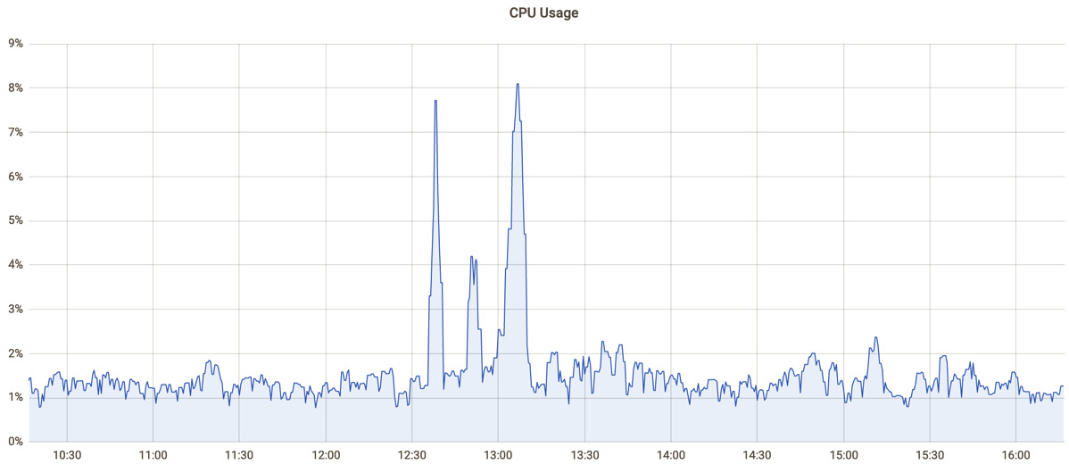
Figure 10.1 – CPU usage metric visualization (X = time, Y = utilization).
While it looks like there been a huge increase in CPU usage between 12:30 to 13:15 according to the graph, the maximum utilization over the period shown was always under 10% suggesting that the system is heavily underutilized. Basic metrics like CPU, memory, or disk usage should always be collected, but often they are not enough to make the right decisions.
Therefore, it is recommended to collect multiple application-specific metrics which could include number of API requests per minute, number of messages waiting in a queue, request response times, number of open connections, and so on. Some of those metrics can be well suited to making right autoscaling decisions and some to provide valuable insights on application performance.
That’s it about metrics for now. Let’s continue with request tracing as next.
Tracing
Is a complete tracking of the requests passing through the components of a distributed system. It allows to see which components are involved in the processing of a particular request, how long the processing takes, and any additional events that happen along. Traces are the results of tracing requests.
Now imagine the following situation. You are investigating longer response times of a distributed, microservice based application you operate, yet the number of requests or load has not changed much. Since most of the application requests traverses’ multiple services, you’ll need to verify each and every service to find the one (or several ones) that are not performing well. However, if you integrate a tracing utility such as Jaeger or Zipkin, it would allow you to trace requests and store and analyze the results. Traces would show which service is having longer response times and might be slowing the whole application down. The traces collected can then be viewed in a dashboard such as the one shown on Figure 10.2 below:

Figure 10.2 – example trace view in Jaeger dashboard.
All-in-all, tracing contributes a lot to observability. It helps to understand the flow of traffic and detect the bottlenecks or issues quickly. Along with logs and metrics, the three telemetry types are a must for monitoring of modern applications and infrastructure. Without those, operators are blind and cannot be sure that all systems are operational and perform as expected. It might take some effort and time to implement the telemetry and observability right, but it always pays off as eventually it will save you a lot of time when it comes to troubleshooting problems.
Speaking about implementation – there is a CNCF project called OpenTelemetry or OTel for short. It provides a set of standardized vendor-agnostic APIs, SDKs and tools to ingest, transform and send data to an observability backend. Support for a large number of open-source and commercial protocols and programming languages (C++, Java, Go, Python, PHP, Ruby, Rust and more) makes it easy to incorporate telemetry into practically any application. It is not strictly required for the scope of KCNA, but if you’d like to know more about it – there will be links in the Further Reading section below.
Moving on, in the next section we’ll learn about Prometheus – number one tool for Cloud Native observability.
Prometheus for monitoring and alerting
After its initial appearance in 2012, Prometheus quickly gained popularity with its rich functionality and Time Series Database (TSDB) that allowed to persisting metrics for querying, analysis, and predictions. Interestingly, Prometheus was inspired by Google’s Borgmon – tool used for monitoring Google’s Borg – the predecessor of Kubernetes.
In 2016, Prometheus was accepted as the second CNCF project (after K8s) that has reached Graduated status by the year 2018. Today, Prometheus is considered an industry standard for monitoring and alerting and widely used with Kubernetes and other CNCF projects.
But enough history, let’s get to the point. First, what is a TSDB?
TSDB
Is a database optimized for storage of data with timestamps. The data could be measurements or events that are tracked and aggregated over time. In case of Prometheus, the data are metrics collected regularly from applications and parts of the infrastructure. The metrics are kept in Prometheus TSDB and can be queried with its own, powerful PromQL query language.
How are the metrics being collected? In general, there are two approaches on collecting monitoring metrics:
- Pull – when a (micro-)service exposes an HTTP endpoint with metrics data, that is periodically scraped (collected) by the monitoring software. Commonly, it is a /metrics URL that is called with a simple HTTP GET request. This is the dominant way how Prometheus works. The service should make the metrics available and keep them up-to-date and Prometheus should make GET requests against /metrics to fetch the data regularly.
- Push – opposite of pull, the service or an application should send the metrics data to the monitoring software. Also supported by Prometheus with Pushgateway and done with HTTP PUT requests. Helpful for the cases when service metrics cannot be scrapped (pulled) due to network restrictions (service behind a firewall or NAT gateway) or simply when the source of the metric has very short lifespan (e.g., quick batch job).
When we say metrics data, it means not just the metric name and value but also a timestamp and often additional labels. Labels indicate certain attributes of a metric and can hold the hostname of a server where the metric was scraped, the name of an application or pretty much anything else. Labels are very helpful for grouping and querying the metrics data with Prometheus’ PromQL language. Let’s see the following metric for an example:
nginx_ingress_controller_requests{
cluster="production",
container="controller",
controller_class="k8s.io/ingress-nginx",
endpoint="metrics",
exported_namespace="kcna",
exported_service="kcnamicroservice",
host="kcnamicroservice.prd.kcna.com",
ingress="kcnamicroservice",
instance="100.90.111.22:10254",
job="kube-system-ingress-nginx-controller-metrics",
method="GET",
namespace="kube-system",
path="/",
pod="kube-system-ingress-nginx-controller-7bc4747dcf-4d246",
prometheus="kube-monitoring/collector-kubernetes",
status="200"} 273175
Here, nginx_ingress_controller_requests is the name of the metric, 273175 is the value of the metric (representing number of requests) and everything else between {} are the labels. As you can see, labels are crucial to narrow down the metric scope, which service it applies to, or what exactly it represents. In this example, it shows the count of HTTP GET requests that were responded with HTTP 200 OK for the service called kcnamicroservice located in kcna namespace.
One other great feature of Prometheus is the dashboard that lets us visualize the data from TSDB directly in the Prometheus UI. While it is very easy to plot graphs with it, its functionality is somewhat limited and that is why many people use Grafana for visualization and metrics analytics.
Now let’s think for a moment how we could collect metrics with Prometheus from applications that we cannot modify? We are talking about services that weren’t developed within your company and the ones that don’t expose the metrics on a /metrics endpoint. This also applies to software that does not come with a webserver such as databases and message buses or even for basic OS stats (CPU, RAM, disk utilization). The solution for such cases is called Prometheus Exporter.
Prometheus Exporter
Is a small tool that bridges the gap between the Prometheus server and applications that don’t natively export metrics. Exporters aggregate custom metrics from a process or a service in the format supported by Prometheus and expose them over /metrics endpoint for collection.
Essentially, an exporter is a minimalistic webserver that knows how to capture metrics from an application that must be monitored and transforms those into Prometheus format for collection. Let’s take PostgreSQL database as an example. Natively it does not expose any metrics, but we can run an exporter along with it that would query the DB and provide observability data that will be pulled into Prometheus TSDB. If run on Kubernetes, the typical way to place an exporter is to put it in the same Pod with the service monitored as a Sidecar container (in case you missed it, Sidecar containers are explained in Chapter 5).
Today, you’ll find a ton of ready-to-use exporters for popular software such as MySQL, Redis, Nginx, HaProxy, Kafka and more. However, if there is no exporter available – it is not a big deal to write one own using any popular programming language with Prometheus client libraries.
Speaking about Kubernetes and Prometheus, there is a seamless integration between the two. Prometheus has out-of-the-box capabilities to monitor Kubernetes and automatically discover the service endpoints of the workloads you run in your K8s cluster. Besides Kubernetes, there is also support for various PaaS and IaaS offerings including those from Google Cloud, Microsoft Azure, Amazon Web Services and many other.
With that, we’ve covered the part about monitoring with Prometheus and before moving on to the alerting, let’s have a look at Figure 10.3 first:

Figure 10.3 – Prometheus architecture.
As you can see, Prometheus server will pull metrics from its targets that can be statically configured or discovered dynamically with service discovery. Short-lived jobs or services behind NAT can also push their metrics via Pushgateway. The metrics can be queried, displayed, and visualized with PromQL in Prometheus web UI or third-party tools.
Moving on, we are going to learn about Prometheus Alertmanager and its notification capabilities.
Alerts
Are reactive elements of a monitoring system triggered by a metric change or a crossing of a certain threshold.
Alerts are used to notify team or an engineer on duty about the change of state in an application or an infrastructure. The notification can take a form of an e-mail, SMS or a chat message as an example. Alertmanager, as you already guessed, is the component of Prometheus responsible for the alerts and notifications.
An alert is normally triggered when a certain metric (or a combination of multiple metrics) has crossed a predefined threshold and stayed above or beyond it for some minutes. Alert definitions are based on Prometheus expression language and accept mathematical operations which allows flexible definition of conditions. In fact, a quite unique feature of Prometheus is the ability to predict when a metric will reach a certain threshold and raise an alert early, before it actually happens. This way, you can define an alert that will notify you five days in advance before a host runs of disk space, as an example. This is possible thanks to Prometheus TSDB that keeps time-series and allows analyzing the data and its rate of change.
Overall, Prometheus is an ultimate solution for monitoring in the Cloud Native era. It is often used to monitor both Kubernetes itself and workloads that run on top of Kubernetes. Today you’ll find plenty of software that supports Prometheus natively by exposing metrics data via /metrics endpoint in the Prometheus format. Client libraries available in many languages make it possible to integrate Prometheus support directly in your own applications. This process is sometimes called direct instrumentation as it introduces native support of Prometheus. For applications and software that does not offer native support, you are likely to find exporters that extract the data and offer it in Prometheus metric format for collection.
Now, some of you probably cannot wait to make hands dirty with Prometheus, but in fact we’ve already covered it in more details than it is required to pass KCNA exam. Nevertheless, you are encouraged to check Further Reading section and try deploying Prometheus onto our miniKube K8s cluster yourself. And for now, we’re moving on to the topic of cost management.
FinOps and cost management
With rapid transition from traditional data centers and collocation towards cloud, it has quickly became apparent that cloud services might be pretty expensive. In fact, if you’d see a bill of a public cloud provider, you’ll often find that everything is metered and everything costs money: cross availability zone traffic and Internet traffic, number of objects or usage of space, number of API requests, Internet IPs, different VM flavors, tiered storage and additional IOPS, storage of VMs that are shut down and the list goes on and on. Sometimes, prices also vary from region to region making it hard to estimate the costs in advance. This has led to the appearance of FinOps in the recent years.
FinOps
Is a cloud financial management discipline and cultural practice. It helps organizations to get the maximum business value based on collaboration of engineering, finance, technology and business teams to make data-driven spending decisions.
Where DevOps puts a lot of focus on collaboration between Development and Operations, FinOps adds Finance to the mix. It helps the teams to manage their cloud spending and stresses the need of collaboration between engineering and business teams as a part of continuous improvement and optimization process. While you don’t need to know the details for the scope of KCNA exam, you’re still encouraged to check about FinOps in the Further Reading section.
When we talk about cloud, by default we assume that we can provision and terminate resources such as virtual machines at any time we want. And we only pay for the time the VM was running. This is known as on-demand capacity or on-demand pricing model, and this is the most popular way to consume cloud services today. You use it – you pay for it, if you’re running nothing – then nothing is charged.
However, there are two more options commonly offered by public cloud providers:
- Reserved instances – These are VMs or bare-metal servers that you reserve for a longer period of time (typically one or more years) and pay the costs up front. Reserved instances come with a very good discount (30-70%) from the regular, on-demand pricing, but you don’t get the same flexibility. Meaning that you’ll keep paying for reserved resources even if you don’t need them.
- Spot instances (sometimes called preemptible instances) – are the instances that can be terminated (deleted) by the cloud provider at any point. Spot instances are leftover and spare capacities that providers offer with huge discounts (60-90%) from on-demand capacity. In some cases, you’ll need to bid (as on auction) for Spot instances and as long as you’re bidding more than the others your instance continues to run.
So, which instance type should you use?
There is no easy answer to this question as there are many variables that come into play and the answer varies from case to case. The rule of a thumb is to buy Reserved instances only for constant workloads or the minimal capacity that is always needed to run your applications. Spot instances can be used for non-critical workloads, batch processing and various non-real-time analytics. Workloads that can be restarted and completed later are a great fit for Spot. And on-demand can be used for everything else including temporarily scaling to accommodate higher loads. As you remember from the previous chapter, Autoscaling is one of the main features of Cloud Native architectures and this is where you’d normally use on-demand instances.
Yet effective cost management in cloud needs more than just right capacity type (on-demand/reserved/spot). The instances should also be of the right size (flavor). This is known as Righsizing.
Rightsizing
Is the continuous process of matching instance size to workload performance and capacity requirements with cost in mind.
We already know that autoscaling is crucial for cost efficiency, and autoscaling can be seen as a part of Rightsizing strategy. You don’t want to run too many underutilized instances when the load is low and the opposite – not having enough instances to handle high load. Autoscaling should target the sweet spot between the capacity/performance and the associated infrastructure costs. But besides the number of instances, their size (number of CPUs, GBs of memory, network throughput, etc.) is also important.
For example, running 40 Kubernetes worker nodes as VMs with only 4 CPUs and 8 GB of RAM might cost you more than running 20 worker nodes with 8 CPUs and 16 GB RAM each despite the same total number of CPUs and RAM. Additionally, many providers offer instances based on different CPU generations and flavors optimized for specific workloads. Some instances might be optimized for high network throughput and some for low-latency disk operations and thus be better suited for your applications. All of that should be taken into consideration as a part of rightsizing strategy and cost management in the cloud.
Summary
In this chapter we’ve learned a lot about Telemetry and Observability. The three telemetry types or signals are logs, metrics and traces which provide valuable insights into the system observed from slightly different perspectives. An observable system is the one that is constantly monitored where we know the state based on the telemetry data that serves as evidence.
We’ve also learned about projects such as OpenTelemetry that can help with instrumentation and simplify the work needed to implement telemetry. Had a quick introduction to projects such as Zipkin and Jaeger for tracing and had a closer look at Prometheus – a fully featured monitoring platform.
Prometheus supports both Push and Pull operating models for metric collection, but dominantly uses Pull model to periodically scrape the metric data at (/metrics endpoint) and save it in TSDB in time-series format. Having metrics in TSDB allows us visualizing the data in software such as Grafana and define alerts that would notify us over the preferred channel when one or another metric is crossing the threshold defined.
Another great point about Prometheus is the Kubernetes integration. Prometheus supports automatic discovery of targets that are running in Kubernetes which makes operator’s life easier. For software that doesn’t natively provide metrics in Prometheus format it is possible to run exporters – small tools that aggregate the metrics from the service or an application and expose them in Prometheus format via /metrics endpoint for collection. If you are in control of the source code of applications you run – it is also possible to add support for Prometheus with a help of client libraries available in many programming languages. This is known as direct instrumentation.
Finally, we’ve got to know about FinOps and cost management in cloud. Most commonly, the so called on-demand capacities are consumed in the cloud. That means resources can be provisioned when needed and deleted when no longer required and only the time when they were running is billed. This is different from Reserved capacity when instances are paid in advance for longer periods of time. Reserved capacities come with very good discounts but will still cost money if unused. And Spot or Preemptible instances are spare capacity that cloud provider might just terminate at any time. They are the cheapest among three options, however, might not be the right choice for critical workloads that require maximum uptime.
Last, but not least, we’ve covered Rightsizing. It’s a process of finding the best instance size and number of instances for current workload as a balance between performance requirements and cost.
Next chapter is about automation and delivery of Cloud Native applications. We will learn about best practices and see how we can ship better software faster and more reliably.
Questions
Correct answers can be found at __TBD__
- Which of the following are valid telemetry signals (pick multiple)?
- Tracks
- Pings
- Logs
- Metrics
- Which is the dominant operation model of Prometheus for metrics collection?
- Push
- Pull
- Commit
- Merge
- Which of the following allows to collect metrics with Prometheus when native application support is missing?
- Running application in Kubernetes
- Installing Pushgateway
- Installing Alertmanager
- Installing application exporter
- Which of the following signals does Prometheus collect?
- Logs
- Metrics
- Traces
- Audits
- Which component can be used to allow applications to push metrics into Prometheus?
- Zipkin
- Grafana
- Alertmanager
- Pushgateway
- Which telemetry signal fits best to see how request traverses a microservice-base application?
- Logs
- Traces
- Metrics
- Pings
- Which software allows visualizing metrics stored in Prometheus TSDB?
- Zipkin
- Kibana
- Grafana
- Jaeger
- Which software can be used for end-to-end tracing of distributed applications (pick multiple)?
- Prometheus
- Grafana
- Jaeger
- Zipkin
- What makes it possible to query Prometheus metrics from the past?
- Alertmanager
- TSDB
- PVC
- Graphite
- Which endpoint Prometheus collects metrics from by default?
- /collect
- /prometheus
- /metric
- /metrics
- What is the format of Prometheus metrics?
- Timeseries
- Traces
- Spans
- Plots
- Which of the following allows direct instrumentation for applications to provide metrics in Prometheus format?
- K8s service discovery
- Pushgateway
- Exporters
- Client libraries
- A periodic job takes only 30 seconds to complete, but Prometheus scrape interval is 60 seconds. What is the best way to collect the metrics from such job?
- push the metrics to Pushgateway
- reduce scrape interval to 30 seconds
- reduce scrape interval to 29 seconds
- replace job with Kubernetes CronJob
- Which of the following is a crucial part of Rightsizing?
- FinOps
- Reserved instances
- Autoscaling
- Automation
- Which of the following should be taken into consideration when implementing Autoscaling?
- CPU utilization metric
- RAM utilization metric
- CPU + RAM utilization metrics
- CPU, RAM, and application specific metrics
- Which of the following instance types are offered by many public cloud providers (pick multiple)?
- On-demand
- Serverless
- Spot
- Reserved
- Which of the following instance types fits for constant workloads with no spikes in load that should run for few years straight?
- On-demand
- Serverless
- Spot
- Reserved
- Which of the following instance types fits for batch processing and periodic jobs that can be interrupted if lowest price is the main priority?
- On-demand
- Serverless
- Spot
- Reserved
Further reading
- OpenTelemetry: https://opentelemetry.io/docs/
- Jaeger: https://www.jaegertracing.io/
- Grafana: https://grafana.com/grafana/
- Prometheus query language: https://prometheus.io/docs/prometheus/latest/querying/basics/
- Prometheus exporters: https://prometheus.io/docs/instrumenting/exporters/
- Kubernetes metrics for Prometheus: https://kubernetes.io/docs/concepts/cluster-administration/system-metrics/
- Introduction to FinOps: https://www.finops.org/