
Chapter 4
Cross-sectional Data Methods
4.1 Overview of General Methods
As the name suggests, cross-sectional data analysis refers to the analysis that looks at the data collected on subjects at one time point, or without regard to time differences (a single-occasion snapshot of the system of variables and constructs), and analyses typically consist of comparing differences between subjects. Even with longitudinal data, cross-sectional analysis is often performed by looking at individual time points. For example, in the IMPACT study described later, investigators randomized patients into two groups and examined depression outcomes at 6 months after baseline to determine if average depression scores differed between the two groups. Many of the missing data methods developed for this setting have been discussed in Chapter 2. Among the recommended approaches that are further described in this chapter, there are four main themes: maximum likelihood approach, Bayesian methods, multiple imputation (MI), and inverse probability weighting (IPW). In addition, we discuss some more advanced techniques such as doubly robust estimators toward the end of the chapter.
4.2 Data Examples
We will illustrate the methods using simulated data as well as data from real-world studies. Three real-world data sets are considered: the NHANES study, the IMPACT study, and the NACC study. The last two examples have already been described in Chapter 1. Next, we briefly describe the simulation study and the NHANES study.
4.2.1 Simulation Study
To illustrate the missing data problems and compare various approaches, we will use simulated data examples with known missing data mechanisms imposed. Scenarios considered will include mixed variable types, missing outcomes only, missing covariates only, and missing both outcomes and covariates.
4.2.2 NHANES Study
We will use a small data set from NHANES with nonmonotone missing values, which has been included as a working example with the R mice package (van Buuren and Groothuis-Oudshoorn, 2011). The data set was first used by Schafer (1997b), and contains 25 observations on the following four variables: age (age group, 1 = 20–39, 2 = 40–59, 3 = 60+), bmi (body mass index, km/m2), hyp (hypertensive, 1 = no, 2 = yes), and chl (total serum cholesterol, mg/dl). The variables age and hyp are considered discrete variables, whereas bmi and chl are treated as continuous variables. We will consider linear models and generalized linear models with bmi and hyp as outcomes.
4.3 Maximum Likelihood Approach
Let Dcom denote the complete-data values in the absence of missing values. We write Dobs and Dmis as the observed and missing parts of Dcom, respectively. We then base our inference on the observed-data likelihood function under the ignorable missing data mechanism. The observed likelihood function can be calculated as follows:
Its score equation can also be obtained as follows:
The maximum likelihood estimator (MLE) for θ can be found by solving the score equation.
In general, there is no closed-form solution for the score equation, and we need to use an iterative method for obtaining a solution for θ. Two commonly used iterative methods are the Newton–Raphson method and the Fischer scoring method. Let θ(t) be the current value of θ after t iterations. The Newton–Raphson method defines the next iteration value θ(t+1) as follows:
where I(θ | Dobs) is the observed information matrix, defined as
where l(θ | Dobs) = log L(θ | Dobs). The Fisher scoring method gives the following iterative value:
where J(θ | Dobs) is the expected information matrix, defined as

A major limitation of these algorithms is that they require computation of the matrix of second derivatives of the log-likelihood. An alternative iterative method is the expectation–maximization (EM) algorithm, which is a general method for finding the MLE with missing data and does not require computation of second derivatives of the observed-data likelihood (Dempster et al., 1977). The basic idea of the EM algorithm for dealing with missing values is that it replaces missing values with estimated values, estimates parameters based on the pseudo-complete data, and iterates through these two steps until convergence. Formally, the EM algorithm consists of an E (expectation) step and an M (maximization) step. An additional advantage of the EM algorithm is that both the E and M steps can oftentimes be easily computed. We now give a mathematical definition of EM.
We let l(θ | Dcom) be the complete-data log-likelihood function. Let θ(t) be the current estimate after t iterations. The t + 1 iteration of the EM algorithm is defined as follows.
- E Step: Compute the conditional expectation of the complete-data log-likelihood function, given the observed data and the current parameter value as follows:

- M Step: Maximize this conditional expected log-likelihood Q(θ | θ(t)) with respect to θ to obtain the next iterative value θ(t+1).
Because we can relate the MLE from the observed-data likelihood to the complete-data likelihood, the EM algorithm has nice theoretical properties. One such property is that every iteration of the EM algorithm increases l(θ|Dobs), that is,
with equality if and only if
This means that the likelihood function increases at every iteration of the EM algorithm until the condition for equality is satisfied and a fixed point of the iteration is reached. If the likelihood is bounded (which might happen in many cases of interest), the EM algorithm yields a nondecreasing sequence, which must converge as the number of iterations goes to infinity. Under fairly general conditions, the resulting fixed point will be the MLE. For proofs and other details, see McLachlan and Krishnan (1998) and Wu (1983). For example, if the likelihood function is unimodal and satisfies a certain differentiability condition, then any EM sequence will converge to the unique maximum likelihood estimate, irrespective of its starting value (Wu, 1983). But for likelihood functions with multiple maxima, convergence might go to a local maximum depending on the starting value.
Although the EM algorithm has nice theoretical properties, it also has some limitations. For example, its convergence is usually much slower than the Newton-Raphson method, and it does not provide a variance–covariance matrix estimate of the resulting MLE. In addition, sometimes the M or E step can be difficult to implement. With today's ever more powerful computing environment, the M step can be easily carried out using existing software packages with increasingly efficient numerical optimization algorithms. The biggest obstacle preventing the EM algorithm from being more widely used when confronted with missing data problems is the difficulty in calculating the expectation of the complete-data likelihood. The original motivation for the EM algorithm is that the complete-data log-likelihood is more tractable than the observed–data log-likelihood. However, for the E step, it is often difficult to find a closed form of the expectation of the complete-data likelihood for many practical problems. Numerical methods such as Laplace approximation and importance sampling can be easily implemented. For more complex distributions, advanced sampling algorithms such as the adaptive rejection sampling technique can be applied. Another situation when the EM algorithm may not be a good option is that when interactions or transformations of variables with missing values are present in the regression. In order to overcome these limitations, some extensions have been proposed, including ECM, AECM, PX-EM, and ECME. See McLachlan and Krishnan (1998) for a detailed description of these extensions.
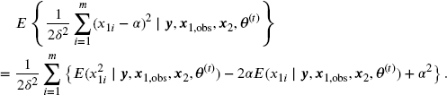
4.3.1 EM Algorithm for Linear Regression with a Missing Continuous Covariate
Now let us demonstrate the EM algorithm with a linear regression model when a continuous covariate is missing. Consider the following regression model:
where ε ~ N(0, σ2). Here, Y and X2 are completely observed, whereas X1 is possibly missing for some subjects. We assume that ![]() . Note that α and δ could be functions of X2 based on the conditional model assumption
. Note that α and δ could be functions of X2 based on the conditional model assumption ![]() . Suppose that we have a simple random sample of size n from model (4.1). Without loss of generality, we assume that the first m subjects have missing X1 values, whereas the remaining subjects are completely observed. Write y = (y1, ..., yn)
. Suppose that we have a simple random sample of size n from model (4.1). Without loss of generality, we assume that the first m subjects have missing X1 values, whereas the remaining subjects are completely observed. Write y = (y1, ..., yn)![]() , x1 = (x11, ..., x1n)
, x1 = (x11, ..., x1n)![]() , x1,mis = (x11, ..., x1m)
, x1,mis = (x11, ..., x1m)![]() , x1,obs = (x1(m+1), ..., xn)
, x1,obs = (x1(m+1), ..., xn)![]() , x2 = (x21, ..., x2n)
, x2 = (x21, ..., x2n)![]() , and θ = (σ, α, δ, β0, β1, β2)
, and θ = (σ, α, δ, β0, β1, β2)![]() . We can formulate the EM algorithm for computing the MLE of θ and the covariance of the MLE. Although the analytic form of the information matrix may be obtained, we will estimate the covariance of the MLE using the observed Fisher information matrix instead.
. We can formulate the EM algorithm for computing the MLE of θ and the covariance of the MLE. Although the analytic form of the information matrix may be obtained, we will estimate the covariance of the MLE using the observed Fisher information matrix instead.
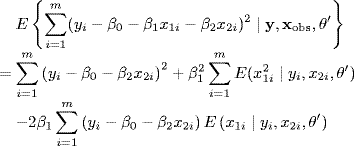
In the E step, we compute

Note that

and
Using the fact that if (X, Y) follows a bivariate normal distribution, ![]() , then
, then ![]() , we have
, we have
and
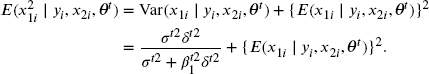
In the M step (maximization), we solve for θ that maximizes Q(θ, θ(t)). Note that the expectations in Q(θ, θ(t)) can be solved by simply replacing missing xmis with their first-and second-order conditional moments. When (Y, X) follows a multivariate normal distribution, using the basic probability distribution theory, the conditional distribution of X | Y is also normal; therefore, the first-and second-order conditional expectation of X | Y can be written in closed form, as already demonstrated. The algorithm for the multivariate normal distribution has been discussed in detail by Schafer (1997b) and Little and Rubin (2002), and has been implemented in R package norm (Schafer, 2013) when (X, Y) are multivariate normal.
4.3.2 EM Algorithm for Linear Regression with Missing Discrete Covariate
Here, we consider the same problem as in Section 4.3.1 except that X1 is discrete. For missing data in multiple discrete covariates, see Ibrahim (1990) and Horton and Laird (1999) for details.
For illustrative purposes, we outline the EM algorithm for binary X1. It can be easily extended to the case where X1 takes more than two discrete values. Let ![]() and
and ![]() . Note that p0 and p1 could be a function of X2. For example,
. Note that p0 and p1 could be a function of X2. For example, ![]() if we assume a logistic regression of X1 on X2. We also let
if we assume a logistic regression of X1 on X2. We also let ![]() . Then, we have
. Then, we have

For the two expectation terms in the above formula, we have
and
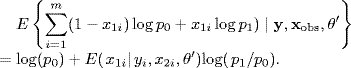
We only need to calculate ![]() , since for binary data
, since for binary data ![]() . Denote Pij '
. Denote Pij ' ![]() P(x1i = j | yi, x2i, θ ') for j = 0, 1. Using Bayes' rule,
P(x1i = j | yi, x2i, θ ') for j = 0, 1. Using Bayes' rule,
This is a special case of the more general weighted EM approach proposed by Ibrahim (1990). It is straightforward to extend the EM algorithm to incorporate auxiliary information; see Horton and Laird (1999) for more information. In the above algorithm, the weights are calculated for values 0 and 1 since the covariate subject to missingness is binary. If the covariate has multiple categories, the weights would be calculated for each possible category of the variable. If two or more discrete covariates have missing values, the weights should be the probability of taking on a specific combination of these covariates conditioning on current parameter estimates.
In the M step, we maximize Q(θ, θ ') with respect to θ. For standard errors and other theoretical properties of the maximum likelihood estimates, see the references mentioned above.
4.3.3 EM Algorithm for Logistic Regression with Missing Binary Outcome
Assume that we observe an independent and identically distributed (i.i.d.) sample of size n, where the binary responses yi ~ Bernoulli(pi) are linked with the vector of covariates xi by a logistic regression model given by
That is,
Then, the full data log-likelihood is
When there are missing outcomes only, the expected full data log-likelihood can be calculated by replacing the expectation with the estimate of the response probability at the current parameter values. We leave this as an exercise to readers.
4.3.4 Simulation Study
Consider a simulation study in which weights and heights of a group of women who exercise at a fitness center are measured. Let Y1 and Y2 denote the measured weight and height, respectively. Further assume that (Y1, Y2) jointly follow a bivariate normal distribution with mean (56.89, 164.71), variance (47.05, 32.03), and covariance 19.91 (correlation 0.51). These values are chosen to resemble the relationship between measured weights (kg) and heights (cm) among a group of exercising females, as reported in Fox (2008), Figure 5.1, page 86. We set that Y1 (weight) is completely observed, whereas Y2 (height) is missing with probability exp (− 0.01Y1)/{1 + exp (− 0.01Y1)}. We can see that Y2 is missing at random (MAR) because the missingness depends on the fully observed Y1 only. Under this setting, we generate a sample of (Y1, Y2) with size 300, the scatter plot of which is given in Figure 4.1.
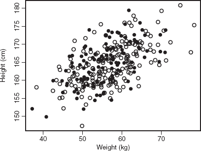
Figure 4.1 Scatter plot of height versus weight. The solid circles are the sample points with height observed, whereas the targets are the sample points with height missing.
We first consider the regression of Y2 on Y1, a missing outcome problem. The results of the full data analysis, complete-case analysis, and the EM algorithm are given in Table 4.1. We can see that the result of the complete-case linear regression is close to that of the full data analysis, implying that the complete-case analysis is unbiased in this case, although there is loss of efficiency due to loss of sample as indicated by the larger standard error estimates. The intercept and slope estimates of the EM algorithm are similar to the full data analysis, with improved standard errors compared to those from the complete-case analysis.
Table 4.1 Linear Regression with Y2 as Outcome
| Coefficient | Full Data | Complete-Case | EM |
| Intercept | 137.75 (2.26) | 138.50 (2.81) | 138.46 (2.20) |
| Weight | 0.47 (0.04) | 0.46 (0.05) | 0.46 (0.04) |
Now we consider the regression of Y1 on Y2, a missing covariate problem. The results are summarized in Table 4.2. We can see that the EM algorithm gives a result similar to that of the full data analysis, whereas the result of the complete-case analysis is quite different from them, meaning that in this case the complete-case analysis is biased.
Table 4.2 Linear Regression with Y2 as Covariate
| Coefficient | Full Data | Complete-Case | EM |
| Intercept | −55.80 (9.41) | −60.39 (12.63) | −54.68 (9.69) |
| Height | 0.68 (0.06) | 0.71 (0.08) | 0.68 (0.06) |
4.3.5 IMPACT Study
As discussed in Chapter 1, the IMPACT study is longitudinal. The primary depression outcome is measured by the Symptom Checklist-20 (SCL-20). For illustrative purposes, we conduct a cross-sectional data analysis looking at the outcomes at the sixth month. The goal is to evaluate the effect of the intervention while controlling for baseline severity. We define a binary outcome, an improvement indicator, which indicates whether there is 50% or more improvement at the sixth month relative to baseline in SCL-20 scores. The group assignment and baseline SCL-20 score are used as covariates, and a logistic regression is considered.
Among the 1797 subjects with observed baseline SCL-20 scores, 1567 subjects are completely observed on the group assignments and the SCL-20 scores at baseline and the sixth month, whereas 230 subjects have their SCL-20 scores at the sixth month missing. A total of 630 subjects have their improvement indicators equal to 1, meaning that they have substantial improvement at the sixth month in SCL-20 scores.
Table 4.3 shows the results of the complete-case analysis and the EM algorithm. It can be seen that the estimates of the two methods are very close, but the estimates of the EM algorithm have smaller standard errors. Although not in all cases, in general the EM algorithm provides more efficient estimates.
Table 4.3 Cross-Sectional Analysis Result for the IMPACT Study
| Complete-Case | EM | |||
| Estimate | SE | Estimate | SE | |
| Intercept | −0.896 | 0.166 | −0.896 | 0.154 |
| Group | 0.803 | 0.106 | 0.803 | 0.099 |
| Baseline SCL-20 | 0.044 | 0.087 | 0.043 | 0.08 |
4.3.6 NACC Study
For illustration, we consider a subset of 400 NACC subjects who died and have complete data on all covariates except neuropathological diagnosis of Alzheimer's disease. A linear regression model considered with continuous outcome MMSE score. The covariates are reaganAD (neuropathological, diagnosis of Alzheimer's disease), age, gender, white, married, stroke, Parkinson's disease (PD), and depression. All variables are binary except the outcome MMSE score and the covariate age. Of the 400 subjects, 273 subject are missing reaganAD. So this is a regression problem with continuous outcome and missing discrete covariate.
The regression analysis results of the complete-case analysis and the EM algorithm are shown in Table 4.4. We can see that there are large differences in coefficient estimates between the EM algorithm and the complete-case analysis.
Table 4.4 Cross-Sectional Analysis Result for the NACC Study
| Complete-Case | EM | |||
| Estimate | SE | Estimate | SE | |
| Intercept | 2.16 | 0.64 | 2.3 | 0.24 |
| reaganAD | 0.97 | 0.28 | 0.77 | 0.16 |
| Cage | −0.15 | 0.14 | 0.04 | 0.08 |
| Gender | −0.04 | 0.31 | −0.53 | 0.16 |
| White | −1.08 | 0.58 | −0.76 | 0.21 |
| Married | 0.27 | 0.33 | 0.51 | 0.17 |
| Stroke | 0.33 | 0.35 | 0.04 | 0.21 |
| PD | 0.26 | 0.59 | 0.15 | 0.33 |
| Depression | 0.36 | 0.37 | −0.07 | 0.24 |
4.4 Bayesian Methods
4.4.1 Theory
In the clinical trials setting, Bayesian methods provide an approach for learning from evidence as it accumulates. In traditional (frequentist) statistical methods, information from the previous studies is used only at the design stage, and never in the formal analysis of the current study. In contrast, in Bayesian methods, Bayes' theorem is used to combine prior information with current information on quantities of interest. This prior information refers to the set of all information that can be used to construct the “prior distribution,” also called the “prior probabilities” or just simply the “prior”.
Bayesian statistical inferences about the parameter θ of interest or missing data Dmis are made in terms of probability statements that are conditional on the observed value Dobs, or p(θ|Dobs) and p(Dmis|Dobs). It is this conditioning on the observed data that makes Bayesian inference different from the traditional (frequentist) statistical inference described in most articles and textbooks, which is based on an evaluation of the procedure used to estimate θ or Dmis over the distribution of possible Dobs values conditional on the true unknown value of θ. Note that in simple settings, results from both methods can be quite similar.
4.4.2 Joint Model and Ignorable Missingness
Let D denote a rectangular data set containing values of several variables. That is, D = (Dij), where Dij is the value of variable j for subject i. We further partition D into observed and missing values, that is, D = {Dobs, Dmis}. Let r = (rij) be the matrix of binary indicator variables such that rij = 1 if Dij is observed, and 0 if Dij is missing. Let α and θ denote vectors of unknown parameters. Then the joint model (likelihood) of the full data is
which often cannot be evaluated in the usual way because it depends on the missing data. However, the marginal distribution of the observed data can be obtained by integrating out the missing data, that is,
There are two commonly used factorizations:
- Selection Model:

- Pattern Mixture Model:

An advantage of the selection model factorization is that it includes the model of interest term directly. On the other hand, the pattern mixture model corresponds more directly to what is actually observed (i.e., the distribution of the data within subgroups having different missing data patterns).
With appropriate conditional independence assumptions, the selection model can be simplified as
Here, f(Dobs, Dmis | θ) is the usual likelihood we would specify if all the data had been observed, and f(r | Dobs, Dmis, α) represents the missing data mechanism and describes the way in which the probability of an observation being missing depends on other variables (observed or not) and/or on its own values. In practice, it is a reasonable assumption that the missing data mechanism and the full data model are specified by distinct parameters. For some types of missing data, the form of the conditional distribution of r can be further simplified.
If data are missing at random, the missing data indicator depends only on the observed data, that is, f(r | Dobs, Dmis, α) = f(r | Dobs, α). So,

If data are missing completely at random (MCAR), f(r | Dobs, Dmis, α) = f(r | α). When α and θ are distinct, the missing indicator r contains no information about θ, and then the inference about θ can be based on f(Dobs | θ) only. The missing data mechanism is termed ignorable if
- the missing data are MCAR or MAR,
- the parameters α and θ are distinct, and
- the priors on α and θ are independent.
Note that when the missingness is ignorable, we can ignore the model of missingness. However, it does not necessarily mean that we can ignore the missing data. In this sense, Bayesian estimation with ignorable missingness is not the same as the available data analysis.
4.4.3 Bayesian Computation for Missing Data
Bayesian analyses are often computationally intensive. However, recent advances in computational algorithms and computing speed have made it possible to carry out calculations for very complex and realistic Bayesian models, increasing the popularity of Bayesian methods (Malakoff, 1999). A basic computational tool is Markov chain Monte Carlo (MCMC) sampling, a method for simulating from the distributions of random quantities.
Algorithmically, Bayesian methods make no distinction between the missing data and the parameters, since both are stochastic (unobserved). Focus is placed on the joint distribution of the missing data and parameters conditional on the observed data, and the typical setup for the joint distribution includes a prior distribution for the parameters, a joint model for all the data (observed and missing), and a model for the missing data process (unless the missing data mechanism is ignorable, in which case this last model is unnecessary).
Missing variables are sampled from their conditional distribution via different methods, such as the Gibbs sampler. There is an imputation stage where simulated draws from the posterior predictive distribution of unobserved values Dmis conditional on observed values Dobs are imputed. Then there is a draw from the posterior distribution of the parameter θ. Inference then proceeds by averaging over the distribution of the missing values. Fully Bayesian methods for missing variables only involve incorporating an extra step in the Gibbs sampler, compared with the case of having no missing values in the data. Therefore, Bayesian methods do not require additional techniques for inference to accommodate missing data. For this reason, Bayesian methods are quite powerful.
Data augmentation (DA), an example of Gibbs sampling, is a Bayesian technique for dealing with missing data under the missing data assumption of ignorability. This procedure is based on iterating between the following two steps. We first take t = 1 and assume that we have a provisional first parameter value θ(1).
- Imputation: This is referred to as the “I step” and imputes the missing data by taking a random draw
 from the conditional distribution L(Dmis|Dobs, θ(t)). The result is called the augmented data set.
 - Posterior: This is referred to as the “P step” and it takes a random draw θ(t+1) from the posterior conditional distribution
 under the assumption that we have no missing data.
This procedure works well in the setting where it is easy to simulate from the posterior distribution if we had the complete data. In theory, as the number of iterations goes to infinity, the distribution of θ(t) converges to the posterior distribution given only Dobs, and the distribution of ![]() converges to the predictive distribution of Dmis given Dobs. But in practice, we must carefully monitor this convergence. This is an example of Gibbs sampling, but there are also Metropolis–Hastings versions of this procedure.
converges to the predictive distribution of Dmis given Dobs. But in practice, we must carefully monitor this convergence. This is an example of Gibbs sampling, but there are also Metropolis–Hastings versions of this procedure.
The above Bayesian model can be implemented using BUGS, WinBUGS, OpenBUGS, or JAGS. WinBUGS is freely available for Windows, OpenBUGS is freely available for both Windows and Linux systems, and JAGS (Just Another Gibbs Sampler) is freely available for Windows, Linux, and Mac OSX (see their web sites for download and installation details).
4.4.4 Simulation Example
Now we consider the data example given in Section 4.3.4. The linear regression of weight on height is considered. To carry out the Bayesian analysis, we need to specify a Bayesian model, which is given by the following BUGS code.
In the above BUGS code, note that in addition to the analysis model that captures the regression relationship, the covariate with missing value is treated as a stochastic node and an imputation model is specified for it. This setup then allows missing values to be simulated from the posterior predictive distributions and uncertainty to be propagated through layers of the joint model. This is the basic idea behind the entire missing data imputation framework.
The regression coefficient estimates from the full data analysis are −55.80 for intercept and 0.68 for slope, while the corresponding posterior means of the Bayesian analysis are −53.68 and 0.67 with standard errors of 11.42 and 0.07, respectively. Results of the Bayesian analysis are very close to those from the full data analysis, but the Bayesian analysis has a larger standard error.
4.4.5 IMPACT Study
For the IMPACT study, the problem involves a regression model with missing binary outcome only. In the following BUGS code, the SCL-20 score at the sixth month is considered a stochastic node and assigned Bernoulli distribution, which then simulates the missing SCL-20 scores using Gibbs sampling.
The Bayesian estimates of the intercept and the coefficients of group assignment and baseline SCL-20 score are −0.896 (0.166), 0.805 (0.106), and 0.043 (0.087), respectively. So we can see that the results of the Bayesian analysis are quite close to those based on the complete-case analysis and EM algorithm.
4.4.6 NHANES Example
We now illustrate the full Bayesian model for missing data in both outcome and covariates, with mixed variable types using the NHANES example included in the mice package. There are 25 subjects in the example with outcome hyp and covariates age, bmi, and chl. The covariate age is completely observed, whereas the other three variables have missing values.
As demonstrated in the following BUGS code, in addition to the analysis model that answers the primary question about the relationship between outcome variable and covariates, there are also two carefully specified imputation models for missing outcomes and missing covariates. Investigators have to take caution to ensure that the imputation models make substantive sense and that there is additional information to be extracted from the observed data to make reasonable imputations.
The Bayesian analysis results are given in Table 4.5. It seems that relative to age and chl, bmi has a stronger relationship with hyp.
Table 4.5 Bayesian Analysis Results for the NHANES Example
| Intercept | Age Group 1 | Age Group 2 | bmi | chl | |
| Mean | −1.466 | −48.195 | 0.248 | 3.048 | −0.135 |
| SD | 3.843 | 20.799 | 0.172 | 1.71 | 31.477 |
4.5 Multiple Imputation
4.5.1 Theory
Instead of replacing each missing value with only one randomly imputed value, it may be more appropriate to replace each with several imputed values that reflect our uncertainty in the imputation model. This is the so-called multiple imputation. Each time we take a set of imputed values separately to form a complete data set. So if we impute five times, we will be able to form five complete data sets. Then, within each of these data sets, we perform a standard analysis (as we would have if there had been no missing values). The final step combines these inferences across data sets. In general, the MI procedure involves the following three steps:
- Imputation: Create M imputations of the missing data,
 , under a suitable model.
 - Analysis: Analyze each of the M complete data sets,
 , m = 1, ..., M, in the same way.
 - Combination: Combine the M sets of estimates and standard errors into a single estimate and standard error using Rubin's rules (Rubin, 1987).
Suppose that we are interested in making inferences about a one-dimensional parameter θ (e.g., a coefficient from a regression model). From each of the M complete data sets, we will obtain estimates ![]() as well as associated variances V1, ..., VM. Using Rubin's rules, for an overall point estimate (also referred to as the combined MI estimator), we simply average over the estimates:
as well as associated variances V1, ..., VM. Using Rubin's rules, for an overall point estimate (also referred to as the combined MI estimator), we simply average over the estimates:
Then the variance of the combined MI estimator involves two components: the average within-imputation variance and the average between-imputation variance. The average within-imputation variance is defined as ![]() , and the average between-imputation variance is defined as
, and the average between-imputation variance is defined as ![]() . These are combined to form the total variance estimator:
. These are combined to form the total variance estimator:
For details on the theoretical justification, see Rubin (1987).
It is assumed that ![]() follows the standard normal distribution for a large sample size and large M. But when the number of imputations M is small, the above normality assumption is questionable. Rubin (1987) and Barnard and Rubin (1999) proposed to replace the normal distribution by a t-distribution for
follows the standard normal distribution for a large sample size and large M. But when the number of imputations M is small, the above normality assumption is questionable. Rubin (1987) and Barnard and Rubin (1999) proposed to replace the normal distribution by a t-distribution for ![]() when M is small. That is,
when M is small. That is,
where the degrees of freedom ![]() . Here,
. Here, ![]() is the relative increase in variance due to missing data. Based on this t-distribution, a 100(1− α) % confidence interval for θ is given by
is the relative increase in variance due to missing data. Based on this t-distribution, a 100(1− α) % confidence interval for θ is given by
and a p-value for testing the null hypothesis θ = θ0 against a two-sided alternative is
or equivalently,
When the complete data sets are based on limited degrees of freedom, say ![]() , an additional refinement replaces ν with
, an additional refinement replaces ν with
where
See Barnard and Rubin (1999) for details.
The MI method has the following advantages: (1) It allows the use of simple complete-data techniques and software once the missing data have been imputed. (2) It allows the data collector (the imputer) and the data analyst to be different. (3) It reflects the sampling variability that occurs from the fact that the values are missing. (4) It reflects uncertainty of the model if the imputations are drawn from different models. (5) It allows one set of imputations drawn in the first step to be used for many different analyses in the second step. In the above description, we did not specify in the first step of MI how to impute the data since there are many different methods. In Chapter 2, we learned that there are some methods for imputation that are better than others. Conventional multiple imputation imputes missing data from the posterior predictive distribution of the missing data, although there are numerous ways to build the imputation model. The conventional method of proposing a multivariate model for mixtures of categorical and continuous data can be problematic, since it is often difficult to propose a sensible joint distribution for all variables of interest. Alternative methods include the use of chained equations, also referred to as regression switching, where a plausible regression model is specified for each univariate variable that must be imputed given all other variables. There are some theoretical shortcomings to this method, since specifying the conditional distributions for each univariate variable does not guarantee a suitable joint model (van Buuren, 2013).
We recommend two approaches for imputing missing values and provide code in Section 4.9 to implement these approaches for multiple imputation. The two approaches are (1) imputation drawing from the posterior predictive distribution and (2) chained equations. There are excellent textbooks dedicated to the MI methods; see Molenberghs and Kenward (2007) and van Buuren (2013).
4.5.2 Some General Guidelines on Imputation Models and Analysis Models
The rules described in the previous section for combining complete-data inferences all assume that the sample is large enough for the usual asymptotic approximations to hold. But for smaller samples, when the asymptotic methods break down, simulation-based summaries of the posterior distribution of θ may be preferable, keeping in mind that Bayesian interpretation depends on a prior distribution.
Parametric Bayesian simulation methods depend heavily on the correct form of the parametric complete-data model. MIs created under a false model may not have a disastrous effect on the final inference, provided the analyses of imputed data sets are done under more plausible assumptions. Because the imputation and analysis steps are distinct, it is possible to have valid MI inferences even if the imputation model is different from the analysis model. The rules for combining complete-data inferences were derived under some implicit assumptions of agreement between these two models.
In the case where the analysis model is a special case of imputation model (i.e., the analyst's model is more restrictive), if the analyst's extra assumptions are true, then MI inferences will be valid. However, they may be conservative since the imputations will reflect an extra degree of uncertainty. If the analyst's extra assumptions are not true, then MI inferences will not be valid.
In the case where the analysis model is more general than the imputation model (i.e., the imputer makes assumptions on the complete data that the analyst does not), if the extra assumptions for imputation models are true, then MI inferences will be still valid. In addition, the MI estimate ![]() will be more efficient than the observed data estimate derived purely from the analysis model because the MI estimate incorporates the imputer's superior knowledge about the data, a property called superefficiency. Moreover, the MI interval will have an average width that is shorter than the confidence interval derived from the observed data and the analyst's model. But if the analyst's extra assumptions are not true, then MI inferences will not be valid.
will be more efficient than the observed data estimate derived purely from the analysis model because the MI estimate incorporates the imputer's superior knowledge about the data, a property called superefficiency. Moreover, the MI interval will have an average width that is shorter than the confidence interval derived from the observed data and the analyst's model. But if the analyst's extra assumptions are not true, then MI inferences will not be valid.
For practical considerations, the imputation model should include
- variables crucial to the analysis,
- variables that are highly predictive of the variables that are crucial to the analysis (e.g., an outcome),
- variables that are highly predictive of missingness, and
- variables that describe special features of the sample design (e.g., for probability surveys).
A general guideline is that the imputer should use a model that is general enough to preserve any associations among variables (two-, three-, or even higher way associations) that may be the target of subsequent analysis. There have been some progress in developing more formal ways of deciding which variables serves as predictors in the imputation model, see the influx and outflux statistics proposed by Van Buuren (2013).
4.5.3 Theoretical Justification for the MI Method
In this section, we outline the theoretical justification for the MI method based on a large-sample Bayesian approximation, which assumes that the observed-data posterior distribution follows a normal distribution. Due to this normal assumption, we can estimate the mean and variance with a much less number of draws needed.
If we assume that p(θ | Dobs) is approximately normal, the observed-data posterior is determined by the posterior mean and variance, E(θ | Dobs) and Var(θ | Dobs). Note that
where the outer expectation is taken with respect to the posterior predictive distribution, p(Dmis | Dobs). By the law of total variance, we have
Furthermore, we can show that

and that

Hence, if ![]() are independent draws of Dmis from the posterior predictive distribution p(Dmis | Dobs), for large M, we have
are independent draws of Dmis from the posterior predictive distribution p(Dmis | Dobs), for large M, we have
where ![]() , the complete-data posterior mean of θ calculated for the mth imputed data set
, the complete-data posterior mean of θ calculated for the mth imputed data set ![]() . Similarly, for large M, we have
. Similarly, for large M, we have
where ![]() is the complete-data posterior variance of θ calculated for the mth imputed data set
is the complete-data posterior variance of θ calculated for the mth imputed data set ![]() , and
, and
where ![]() . We call
. We call ![]() and B the average within-imputation variance and between-imputation variance, respectively.
and B the average within-imputation variance and between-imputation variance, respectively.
4.5.4 MI When θ Is k-Dimensional
When θ is not a scalar, but a vector with k dimensions, finding an adequate reference distribution for the statistic
is not a simple task. The main problem is that for small M, the between-imputation covariance matrix B is a poor estimate of V(θ | Dobs), and does not even have full rank if M ≤ k. One solution is to make the assumption that the population between-and within-imputation covariance matrices are proportional to one another, which is equivalent to assuming that the fractions of missing information for all components of θ are equal. Under this assumption, a more stable estimator of total variance is
where ![]() is the average relative increase in variance due to the missing data across the components of θ, and tr
is the average relative increase in variance due to the missing data across the components of θ, and tr![]() is the trace of
is the trace of ![]() , the sum of main diagonal elements of
, the sum of main diagonal elements of ![]() .
.
Under the null hypothesis H0 : θ = θ0, the test statistic
follows an F-distribution with the degrees of freedom k and ν1. Hence, the p-value is ![]() . For k(M − 1) > 4, the degrees of freedom are
. For k(M − 1) > 4, the degrees of freedom are
For k(M − 1) ≤ 4, the degrees of freedom are
Although the above reference distribution is derived under the strong assumption that the fractions of missing information for all components of θ are equal, Li et al. (1991) reported encouraging results even when this assumption is violated.
Assume that there are nuisance parameters ϕ, in addition to the parameter of interest θ. Our null and alternative hypotheses are H0 : θ = θ0 versus H1 : θ ≠ θ0. Let ![]() and
and ![]() be the estimates of θ and ϕ without H0, and let
be the estimates of θ and ϕ without H0, and let ![]() be the estimate of ϕ under H0 when there are no missing data. Then, the p-value for θ = θ0 based on the likelihood ratio test will be
be the estimate of ϕ under H0 when there are no missing data. Then, the p-value for θ = θ0 based on the likelihood ratio test will be ![]() , where
, where ![]() and
and ![]() is a χ2 random variable with k degrees of freedom.
is a χ2 random variable with k degrees of freedom.
For the mth imputed data set ![]() , let
, let ![]() be the estimates of θ and ϕ without assuming H0 and
be the estimates of θ and ϕ without assuming H0 and ![]() be an estimate of ϕ under H0 : θ = θ0, and LR(i) be the corresponding likelihood ratio test statistic. Let
be an estimate of ϕ under H0 : θ = θ0, and LR(i) be the corresponding likelihood ratio test statistic. Let ![]() ,
, ![]() ,
, ![]() , and
, and ![]() . Assume that the function LR can be evaluated for each of the M complete data sets at
. Assume that the function LR can be evaluated for each of the M complete data sets at ![]() , θ0, and
, θ0, and ![]() to obtain M values of LR
to obtain M values of LR![]() whose average across the m imputations is
whose average across the m imputations is ![]() . Then, the test statistic
. Then, the test statistic
has the same asymptotic distribution as ![]() (Meng and Rubin, 1992). Hence, the p-value is
(Meng and Rubin, 1992). Hence, the p-value is ![]() .
.
In some cases, the complete-data method may not produce estimates of the general function LR(·), but only the value of the likelihood ratio statistic. So if we do not have ![]() but only LR1, ..., LRm, then there is a less accurate way to combine this value (Li et al., 1991). The repeated-imputation p-value is given by
but only LR1, ..., LRm, then there is a less accurate way to combine this value (Li et al., 1991). The repeated-imputation p-value is given by
where
ν is the sample variance of ![]() , and
, and
4.5.5 Simulated Example
In the simulated data, weight is fully observed, whereas height contains some missing values. We carry out MI by sampling the missing values from the predictive distribution based on the complete-case regression model. We also carry out the mean imputation that imputes the missing values by the mean of the predictive distribution. Results are shown in Table 4.6. It can be seen that the mean imputation does not work well, while MI gives results similar to those of the full data analysis.
Table 4.6 Regression Analysis for the Cross-Sectional Simulated Data Based on Imputation Methods
| Mean Imputation | MI | |||
| Estimate | SE | Estimate | SE | |
| Intercept | −99.32 | 10.34 | −56.13 | 10.44 |
| Height | 0.95 | 0.06 | 0.69 | 0.06 |
4.5.6 IMPACT Study
We carry out multiple imputation for the IMPACT study by predictive mean matching with chained equations. Note that passive imputation for the binary outcome is involved. The estimates of the intercept and the coefficients of the group assignment and baseline SCL-20 score are −0.832(0.16), 0.857(0.10), and −0.008(0.09), respectively, which are close to the results obtained by the EM algorithm and the Bayesian analysis.
4.6 Imputing Estimating Equations
The idea of imputing the estimating equations was first proposed by Paik (1997). It is also called the mean score imputation because the estimating equations are often constructed by the score functions. With the full data, suppose that we can use some estimating equations to estimate the parameter of interest θ; that is, we look for an estimate of θ by solving the following estimating equation:
where Di is the full data of subject i. When there is possibility of missing some values of subject i, Di can be further partitioned into the observed part Dobs,i and the missing part Dmis,i. When some elements of Di are missing, we can use the expectation of U(Di; θ) as an “imputation”:
where the expectation is taken with respect to Dmis,i given Dobs,i. This estimator would be similar to the multiple imputation proposed by Wang and Robins (1998), which uses the following estimating equation:
where ![]() is a realization from the conditional distribution
is a realization from the conditional distribution ![]() . Fay (1996) proved that this estimator has the same asymptotic behavior as the traditional multiple imputation estimator. It is obvious that as m is large,
. Fay (1996) proved that this estimator has the same asymptotic behavior as the traditional multiple imputation estimator. It is obvious that as m is large, ![]() would be close to
would be close to ![]() . Therefore, the imputed estimating equation can be regarded as a limiting case of the multiple imputation.
. Therefore, the imputed estimating equation can be regarded as a limiting case of the multiple imputation.
If the full data estimating equation is consistent, that is, ![]() , then the imputed estimating equation is also consistent, because
, then the imputed estimating equation is also consistent, because
In practice, an imputation model is usually needed to estimate the conditional expectation ![]() .
.
4.7 Inverse Probability Weighting
4.7.1 Theory
When missing data mechanism is not missing completely at random, the subjects with complete observations often constitute a biased sample of the study population. The inverse probability weighting (IPW) method uses the idea of weighting each complete case back to the original population, and is commonly used in survey sampling. Its main advantage is its semiparametric nature and flexibility. Suppose that we observe the following data:
| Group | Exposed | Non-exposed |
| Response | 1 1 1 1 | 2 2 2 2 |
Then the average response is 1.5. If instead we only observe one subject in the exposed group and three subjects in the non-exposed group, then the average response of those observed is 7/4 = 1.75, which is biased. Note that the probability of response is 1/4 in the exposed group and 3/4 in the not exposed group. We can therefore calculate a weighted average, where each observation is weighted by the inverse of probability of being observed. Specifically, the weighted average is
Thus, in this case, IPW has eliminated the bias through “constructing” the full population by weighting the data from subjects who have a certain probability of being observed. More generally, it can be shown that the IPW estimators are unbiased and consistent.
We now apply this idea to the problem of estimating equations with missing observations. Let Ri denote the missingness indicator, where Ri = 1 if subject i is completely observed, and 0 otherwise. Let Dobs,i and Di be the observed and full data of subject i, respectively. Define ![]() . The IPW estimating equation is then given as follows:
. The IPW estimating equation is then given as follows:
where ![]() . After weighting each of the complete cases by the inverse of selection probability, the estimating equations would be consistent by noting that
. After weighting each of the complete cases by the inverse of selection probability, the estimating equations would be consistent by noting that

In practice, the missingness mechanism π(Dobs,i) is either known by design or must be estimated from some parametric model. In the latter case, the IPW estimator requires the correct specification of the missingness mechanism model. Technically, it is also required that the selection probability is strictly positive, that is, π(Dobs,i) > 0. If some subjects are observed with very small probabilities, then the IPW estimator could be very inefficient and even unstable.
4.7.2 Simulated Example
Consider the linear regression of weight on height. The estimates of the intercept and the coefficient of height are −59.96 (12.68) and 0.71 (0.08), respectively. Compared with the complete-case analysis, we can see that the IPW substantially reduces the bias of the estimates.
4.8 Doubly Robust Estimators
4.8.1 Theory
The IPW estimator does not make full use of the available data, since the subjects with missing data are removed. Robins et al. (1994, 1995) first proposed the doubly robust (DR) estimator to improve the efficiency of the IPW estimator. Here, we focus only on the missingness of one variable. Suppose that we could partition Di into
where only the scalar ![]() is subject to missingness and
is subject to missingness and ![]() is observed for everybody. It should be noted that
is observed for everybody. It should be noted that ![]() could be either an outcome or a covariate. The doubly robust estimator is obtained by solving the following estimating equation:
could be either an outcome or a covariate. The doubly robust estimator is obtained by solving the following estimating equation:
Usually both ![]() and
and ![]() need to be estimated from the data. So, the inference would incorporate the knowledge from both the missingness mechanism and the imputation model. The most attractive feature of (4.2) is that the estimating equation is consistent if either the imputation model or the missingness mechanism model is correct, but not necessarily both.
need to be estimated from the data. So, the inference would incorporate the knowledge from both the missingness mechanism and the imputation model. The most attractive feature of (4.2) is that the estimating equation is consistent if either the imputation model or the missingness mechanism model is correct, but not necessarily both.
If the missingness mechanism model is correct,

If the imputation model is correct,

When more than one variables are subject to missingness, the doubly robust estimators usually have a more complicated form. Interested readers should refer to Tsiatis (2006).
4.8.2 Variance Estimation
The imputation, IPW, and DR estimators often involve the estimation of nuisance parameters in order to evaluate π(Dobs,i) and/or ![]() . So before introducing the variance estimate for
. So before introducing the variance estimate for ![]() , we need to discuss the estimation of the nuisance parameters.
, we need to discuss the estimation of the nuisance parameters.
The estimation of π(Dobs,i) can be obtained from a binary regression of Ri on some design matrix W1i, which is expanded by the observed variables Dobs,i. For example, we can assume that
where η1 is the nuisance parameter in the selection model.
The estimation of ![]() is usually less straightforward. But if the full data estimating function U(Di; θ) is linear in Dmis,i, then we only need to model
is usually less straightforward. But if the full data estimating function U(Di; θ) is linear in Dmis,i, then we only need to model ![]() . In the following cases, U(Di; θ) would be linear in Dmis,i: (a) missing categorical variables; or (b) missing continuous outcome. Then, we may estimate
. In the following cases, U(Di; θ) would be linear in Dmis,i: (a) missing categorical variables; or (b) missing continuous outcome. Then, we may estimate ![]() from regression models. For example, a natural choice is generalized linear models
from regression models. For example, a natural choice is generalized linear models
where W2i is the design matrix and η2 is the nuisance parameter in the imputation model. When U(Di; θ) is nonlinear in Dmis,i,
which requires additional steps to estimate the density function ![]() .
.
Now we write S2(η) = ∑ iS2i(η) to be the estimating equation for the imputation model and/or the selection model, and S1(θ, η) = ∑ iS1i(θ, η) to be the estimating equation of the imputation, IPW, or DR estimators. Under some mild regularity conditions, ![]() follows a normal distribution asymptotically, with the sandwich-form variance:
follows a normal distribution asymptotically, with the sandwich-form variance:
where
In practice, we evaluate I and A by replacing E(·) with the sample mean ![]() .
.
4.8.3 NACC Study
We fit the linear regression of the MMSE score (Y) versus the risk factors (X), true disease status (D), and the interaction between the disease status and the risk factors (D × X). So the model is
We also allow the variance of the MMSE score to differ for AD and non-AD subjects:
The MMSE score is transformed to ![]() and the age is transformed to (age − 70)/10, so that the reported coefficients are of the appropriate magnitude. All the risk factors, as well as the MMSE score, are included in the missingness mechanism model. The imputation model also includes the quadratic term of the test score, as well as the interaction between the test and the covariates.
and the age is transformed to (age − 70)/10, so that the reported coefficients are of the appropriate magnitude. All the risk factors, as well as the MMSE score, are included in the missingness mechanism model. The imputation model also includes the quadratic term of the test score, as well as the interaction between the test and the covariates.
The results are shown in Table 4.7. The results from the three methods generally coincide with each other. The DR estimator identifies the main effects of race, clinical AD, and true disease status to be significant, indicating that these variables affect the magnitude of the test score. The race × D interaction is significant, whereas gender, clinical AD, and depression have marginally insignificant interactions with D.
Table 4.7 The Estimated Location and Scale Parameters with the Associated Standard Errors for the NACC Data
| DR | IPW | IB | |
| Intercept | 1.394 (0.125) | 1.452 (0.199) | 1.408 (0.131) |
| Age | −0.064 (0.039) | −0.114 (0.051) | −0.054 (0.032) |
| Gender | −0.049 (0.079) | 0.046 (0.096) | −0.028 (0.074) |
| Race | −0.303 (0.131) | −0.525 (0.203) | −0.304 (0.128) |
| Marital status | 0.083 (0.086) | 0.219 (0.102) | 0.031 (0.076) |
| Clinical AD | 1.120 (0.077) | 1.160 (0.097) | 1.128 (0.070) |
| Stroke | 0.129 (0.095) | 0.100 (0.125) | 0.129 (0.083) |
| Parkinson's | 0.186 (0.138) | 0.228 (0.153) | 0.292 (0.124) |
| Depression | −0.007 (0.108) | 0.144 (0.156) | −0.006 (0.083) |
| D | 0.984 (0.167) | 1.090 (0.250) | 0.982 (0.170) |
| D × Age | 0.049 (0.052) | 0.085 (0.063) | 0.035 (0.041) |
| D × Gender | −0.146 (0.099) | −0.065 (0.119) | −0.180 (0.090) |
| D × Race | −0.322 (0.158) | −0.339 (0.240) | −0.330 (0.152) |
| D × Marital status | 0.039 (0.108) | −0.090 (0.127) | 0.110 (0.094) |
| D × Clinical AD | −0.150 (0.106) | −0.154 (0.127) | −0.166 (0.095) |
| D × Stroke | −0.124 (0.120) | −0.082 (0.156) | −0.115 (0.105) |
| D × Parkinson's | 0.074 (0.172) | 0.012 (0.190) | −0.058 (0.155) |
| D × Depression | −0.225 (0.135) | −0.119 (0.180) | −0.153 (0.102) |
4.9 Code Used in This Chapter
4.9.1 Code Used in Section 4.3.4
The following code is used to generate a sample of (Y1, Y2) with size 300, where Y1 is completely observed, and Y2 is missing with probability exp (− 0.01Y1)/{1 + exp (− 0.01Y1)}:
> require(MASS) # mvrnorm> set.seed(1235813)> N <- 300 # the sample size> S <- matrix(c(47.05, 19.94, 19.94, 32.03), 2, 2)> dd <- data.frame(mvrnorm(N, c(56.89, 164.71), S))> colnames(dd) <- c(”weight”, ”height”)> pmis <- expit(-0.01, dd $dollar $ weight)> drop <- rbinom(N, 1, pmis) # about 36> simu <- data.frame(cbind(dd, drop))
The following code is used to carry out the full data analysis, complete-case analysis, and EM algorithm of regression of Y2 on Y1:
## full data analysis> lm(height ~ weight, data = simu)## complete-case analysis> lm(height ~ weight, data = simu, subset = !drop)## EM algorithm# prepare data> y <- simu $dollar $ height> r.y <- drop> y[r.y == 1] <- NA> X <- cbind(1, simu $dollar $ weight)> fit <- lm(y ~ X[, 2])> d <- summary(fit)> theta.hat <- c(d $dollar $ sigma, d $dollar $ coef[, 1])# theta.hat is the initial values from ols estimates# iterate over EM steps> n.iter <- 0> diff <- 10> theta.hat <- rep(0.5, 3) # starting values> while (diff >= 1e-06 & n.iter < 20) {+ my.em <- optim(theta.hat, method = ”L-BFGS-B”,+ fn = eloglik.cy.my, gr = eloglik.cy.my.gradient,+ hessian = TRUE, lower = c(1e-06, -Inf, -Inf),+ upper = rep(Inf, 3), y = y,+ r.y = r.y, X = X, theta.hat = theta.hat)+ diff <- abs(max(my.em $dollar $ par - theta.hat))+ n.iter <- n.iter + 1+ theta.hat <- my.em $dollar $ par+ }> inverted <- solve(my.em $dollar $ hessian)> tval <- my.em $dollar $ par/sqrt(diag(inverted))> pval <- 2 * (1 - pt(abs(tval), nrow(X) - ncol(X)))> results <- cbind(my.em $dollar $ par, sqrt(diag(inverted)), tval, pval)> colnames(results) <- c(”Estimate”, ”Std. Error”, ”t value”,+ ”Pr(>| t| )”)> rownames(results) <- c(”sigma”, ”Intercept”, ”weight”)> print(results)
The following code is used to carry out the full data analysis, complete-case analysis, and EM algorithm for the regression of Y1 on Y2:
## Full data analysis> lm(weight ~ height, data = simu)## complete-case analysis> lm(weight ~ height, data = simu, subset = !drop)## EM algorithm# prepare data> y <- simu $dollar $ weight> x <- simu $dollar $ height> x[simu $dollar $ drop == 1] <- NA> X <- cbind(1, x)> r.x <- simu $dollar $ drop> d <- summary(lm(weight ~ height, data = simu, subset = !drop))> theta.cc <- c(d $dollar $ sigma, mean(X[, 2], na.rm = T),+ sd(X[, 2], na.rm = T), d $dollar $ coef[, 1])# theta.cc is the initial value for EM iterations# iterate over EM steps> n.iter <- 0> diff <- 10> theta.hat <- rep(0.5, 5) # try different starting values> while (diff > 1e-06 & n.iter < 50) {+ my.em <- optim(theta.hat, method = ”L-BFGS-B”,+ fn = eloglik.cycx.mx, hessian = TRUE,+ lower = c(1e-06, -Inf, 1e-06, rep(-Inf, 2)),+ upper = rep(Inf, 5), y = y, X = X, r.x = r.x,+ mXcol = 2, theta.hat = theta.hat)+ diff <- abs(max(my.em $dollar $ par - theta.hat))+ n.iter <- n.iter + 1+ theta.hat <- my.em $dollar $ par+ }> inverted <- solve(my.em $dollar $ hessian)# numeric hessian is not quite stable> se <- sqrt(diag(inverted))> tval <- my.em $dollar $ par/se> pval <- 2 * (1 - pt(abs(tval), nrow(X) - ncol(X)))> results <- cbind(my.em $dollar $ par, se, tval, pval)> colnames(results) <- c(”Estimate”, ”Std. Error”, ”t value”,+ ”Pr(>| t| )”)> rownames(results) <- c(”sigma”, ”m.x”, ”sd.x”, ”Intercept”,+ ”height”)
4.9.2 Code Used in Section 4.3.5
The following code is used to carry out the complete-case analysis and the EM algorithm for the IMPACT data:
## complete-case analysis> y <- impact $dollar $ respond> r.y <- is.na(y)> y[r.y == 1] <- NA> X <- cbind(1, impact $dollar $ group, impact $dollar $ scl.0)> d <- summary(glm(respond ~ group + scl.0, data = impact,+ family = binomial(link = ”logit”), na.action = ”na.omit”))## iterate over EM steps> n.iter <- 0> diff <- 10> theta.hat <- rep(0.5, 3)# the above code is to try different starting values> while (diff > 1e-06 & n.iter < 50) {+ my.em <- optim(theta.hat, method = ”L-BFGS-B”,+ fn = eloglik.dy.my, hessian = TRUE,+ lower = rep(-Inf, 3), upper = rep(Inf, 3),+ y = y, r.y = r.y, X = X, theta.hat = theta.hat)+ diff <- abs(max(my.em $dollar $ par - theta.hat))+ n.iter <- n.iter + 1+ theta.hat <- my.em $dollar $ par+ }> inverted <- solve(my.em $dollar $ hessian)> tval <- my.em $dollar $ par/sqrt(diag(inverted))> pval <- 2 * (1 - pt(abs(tval), nrow(X) - ncol(X)))> results <- cbind(my.em $dollar $ par, sqrt(diag(inverted)), tval, pval)> colnames(results) <- c(”Estimate”, ”Std. Error”, ”t value”,+ ”Pr(>| t| )”)> rownames(results) <- c(”Intercept”, ”group1”, ”scl.0”)
4.9.3 Code Used in Section 4.4.4
The following code is used to carry out the Bayesian analysis for the simulation example:
# THE DATA> X <- c(simu $dollar $ height) # get rid of attributes> Y <- c(simu $dollar $ weight)> X[simu $dollar $ drop == 1] <- NA> N <- length(Y)> dataList <- list(X = X, Y = Y, N = N)> ii <- min(c(1:N)[is.na(X)]) # first missing value to monitor
# THE ARGUMENTS# The parameters to be monitored> parameters <- c(”b[1]”, ”b[2]”, paste0(”X[”, ii, ”]”))# Number of steps to ’tune’ the samplers.> adaptSteps <- 1000# Number of steps to ’burn-in’ the samplers.> burnInSteps <- 5000# Number of chains to run.> nChains <- 3# Total number of steps in chains to save.> numSavedSteps <- 10000# Number of steps to ’thin’ (1=keep every step).> thinSteps <- 10# Steps per chain.> nIter <- ceiling((numSavedSteps * thinSteps)/nChains)
# Require R package rjags/runjags and JAGS package!require(rjags)
# export model specification to an external text file> writeLines(modelString, con = ”mymodel.bug”)
# Create, initialize, and adapt the model:> jagsModel <- jags.model(”mymodel.bug”, data = dataList,+ n.chains = nChains, n.adapt = adaptSteps)
# Burn-in:> cat(”Burning in the MCMC chain... ”)> update(jagsModel, n.iter = burnInSteps, progress.bar = ”none”)
# The saved MCMC chain:> cat(”Sampling final MCMC chain... ”)> codaSamples <- coda.samples(jagsModel, variable.names+ = parameters, n.iter = nIter, thin = thinSteps)
# EXAMINE THE RESULTS.> checkConvergence <- T> if (checkConvergence) {+ show(summary(codaSamples))+ }
4.9.4 Code Used in Section 4.4.5
The following code is used to carry out the Bayesian analysis for the IMPACT study:
# THE DATA> respond <- c(impact $dollar $ respond) # get rid of attributes> group <- c(impact $dollar $ group)> scl.0 <- c(impact $dollar $ scl.0)> N <- length(respond)> dataList <- list(respond = respond, group = group,+ scl.0 = scl.0, N = N)# first missing value to monitor> ii <- min(c(1:N)[is.na(respond)])
# THE ARGUMENTS# The parameters to be monitored> parameters <- c(”b[1]”, ”b[2]”, ”b[3]”,+ paste0(”respond[”, ii, ”]”))# Number of steps to ’tune’ the samplers.> adaptSteps <- 1000# Number of steps to ’burn-in’ the samplers.> burnInSteps <- 5000> nChains <- 3 # Number of chains to run.# Total number of steps in chains to save.> numSavedSteps <- 5000# Number of steps to ’thin’ (1=keep every step).> thinSteps <- 10# Steps per chain.> nIter <- ceiling((numSavedSteps * thinSteps)/nChains)
> require(rjags)
# export BUGS model to an external text file> writeLines(modelString, con = ”mymodel.bug”)
# Create, initialize, and adapt the model:> jagsModel <- jags.model(”mymodel.bug”, data = dataList,+ n.chains = nChains, n.adapt = adaptSteps)
# Burn-in:> cat(”Burning in the MCMC chain... ”)> update(jagsModel, n.iter = burnInSteps, progress.bar = ”none”)
# The saved MCMC chain:> cat(”Sampling final MCMC chain... ”)> codaSamples <- coda.samples(jagsModel,+ variable.names = parameters,+ n.iter = nIter, thin = thinSteps)
4.9.5 Code Used in Section 4.4.6
The following code is used to carry out the Bayesian analysis for the NHANES example:
# THE DATA> age.gp1 <- ifelse(c(nhanes2 $dollar $ age) == 1, 1, 0)> age.gp2 <- ifelse(c(nhanes2 $dollar $ age) == 2, 1, 0)# change to 0/1, and get rid of attributes> hyp <- c(nhanes2 $dollar $ hyp) - 1> bmi <- c(nhanes2 $dollar $ bmi)> chl <- c(nhanes2 $dollar $ chl)> N <- length(hyp)> dataList <- list(hyp = hyp, age.gp1 = age.gp1,+ age.gp2 = age.gp2, bmi = bmi, chl = chl, N = N)
# THE ARGUMENTS# The parameters to be monitored> parameters <- c(”b[1]”, ”b[2]”, ”b[3]”, ”b[4]”, ”b[5]”)# Number of steps to ’tune’ the samplers.> adaptSteps <- 1000# Number of steps to ’burn-in’ the samplers.> burnInSteps <- 5000> nChains <- 3 # Number of chains to run.# Total number of steps in chains to save.> numSavedSteps <- 5000# Number of steps to ’thin’ (1=keep every step).> thinSteps <- 10# Steps per chain.> nIter <- ceiling((numSavedSteps * thinSteps)/nChains)
# Export bugs model to external text file> writeLines(modelString, con = ”mymodel.bug”)
# Create, initialize, and adapt the model:> jagsModel <- jags.model(”mymodel.bug”, data = dataList,+ n.chains = nChains, n.adapt = adaptSteps)
# Burn-in:> cat(”Burning in the MCMC chain... ”)> update(jagsModel, n.iter = burnInSteps, progress.bar = ”none”)
# The saved MCMC chain:> cat(”Sampling final MCMC chain... ”)> codaSamples <- coda.samples(jagsModel,+ variable.names = parameters,+ n.iter = nIter, thin = thinSteps)
4.9.6 Code Used in Section 4.5.5
The following code is used to carry out the analysis based on the mean imputation and the multiple imputation:
# fit a model on height using available data> impmodel <- lm(height ~ weight, data = simu, subset = !drop)# replace missing height with predicted values> simu $dollar $ height.imp <- ifelse(simu $dollar $ drop,+ predict(impmodel, newdata = simu), simu $dollar $ height)# multiple imputation> dd1 <- simu> sigma <- summary(impmodel) $dollar $ sigma# s is residual standard error from impmodel> dd1 $dollar $ height <- ifelse(drop, rnorm(nrow(simu),+ m = predict(impmodel, newdata = simu), s = sigma),dd $dollar $ height)> dd2 <- simu> dd2 $dollar $ height <- ifelse(drop, rnorm(nrow(simu),+ m = predict(impmodel, newdata = simu), s = sigma),dd $dollar $ height)> dd3 <- simu> dd3 $dollar $ height <- ifelse(drop, rnorm(nrow(simu),+ m = predict(impmodel, newdata = simu), s = sigma),dd $dollar $ height)> dd4 <- simu> dd4 $dollar $ height <- ifelse(drop, rnorm(nrow(simu),+ m = predict(impmodel, newdata = simu), s = sigma),dd $dollar $ height)> dd5 <- simu> dd5 $dollar $ height <- ifelse(drop, rnorm(nrow(simu),+ m = predict(impmodel, newdata = simu), s = sigma),dd $dollar $ height)> library(mitools) # to combine imputed data> ddimp <- imputationList(list(dd1, dd2, dd3, dd4, dd5))> models <- with(ddimp, lm(weight ~ height))
4.9.7 Code Used in Section 4.5.6
The following code is used to multiply impute missing value using predictive mean matching, involving passive imputation:
> impact.imp <- mice(impact, method = c(rep(”pmm”, 4),+ ”~ifelse((scl.6-scl.0) <= -scl.0/2, 1, 0”,+ ”~scale(scl.6)”), printFlag = FALSE)> fit <- with(impact.imp, glm(respond ~ group + scl.0,+ family = binomial))> pool(fit)
4.9.8 Code Used in Section 4.7.2
The following code is used to carry out the IPW estimation for the simulated data example:
# estimate the probability of being observed> pmodel <- glm(drop ~ weight, data = simu, family = binomial)> estp <- 1 - fitted(pmodel)# weighted results> s <- lm(weight ~ height, data = simu, subset = !drop,+ weights = 1/estp)