
Chapter 8
Analysis of Randomized Clinical Trials with Noncompliance
8.1 Overview
In previous chapters, we introduced various methods for dealing with missing data. In this chapter, we apply some of these methods to make causal inference in randomized clinical trials with noncompliance and possibly missing outcome data.
A randomized clinical trial is the established gold standard for assessing the causal effect of a new intervention on patient outcomes. The validity of using a simple comparison of outcomes across intervention and control groups to estimate the causal effect of the intervention versus control depends on the assumption that the randomized experiment is implemented perfectly as designed. However, in practice, due to various reasons, many violations of the randomization protocol occur, and one of them is noncompliance, which occurs when the actual treatment a patient takes is different from the initially assigned treatment. Although on the surface it seems that the causal inference of randomized clinical data with noncompliance has nothing in common with the analysis of missing data, it turns out that techniques for dealing with missing data can also be adapted to estimate causal effects with randomized clinical data with noncompliance.
In practice, we encounter two types of noncompliance: (1) all-or-none noncompliance (e.g., either compliant or not) and (2) partial noncompliant. Since most of the available methods in the literature are for all-or-none compliance, in this chapter we focus on the problem of all-or-none compliance. For methods dealing with partial noncompliance, we refer readers to the following references: Efron and Feldman (1991), Goetghebeur and Molenberghs (1996), Goetghebeur et al. (1998), and Jin and Rubin (2008).
For dealing with the problem of all-or-none compliance, there are four different classes of methods available: instrumental variables (IV) methods, moment-based methods, likelihood-based methods, and Bayesian methods. For example, Angrist et al. (1996) and Imbens and Rubin (1997b) proposed nonparametric methods for the causal analysis of studies with noncompliance using the idea 187 of instrumental variables. Cuzick et al. (1997) developed likelihood methods for the causal analysis of studies with all-or-none compliance. Rubin (1974) and Imbens and Rubin (1997a) developed likelihood and Bayesian methods for the causal analysis of single follow-up studies without covariates; Hirano et al. (2000) extended their Bayesian methods to the single follow-up studies when the outcomes and compliance behavior might depend on some observed covariates.
In some clinical trials, subjects may also be missing their outcomes in addition to the problem of noncompliance. Several methods have also been developed to deal with both the problem of noncompliance and missing data. In general, two types of methods have been proposed, depending on how to model the missing data mechanism. One is based on the assumption that the missing data mechanism is latent ignorable (Frangakis and Rubin, 1999; Zhou and Li, 2006; Taylor and Zhou, 2009a, 2009b), and the other one is based on the nonignorable assumption (Chen et al., 2009).
This chapter is organized as follows. In Section 8.2, we introduce two real-world randomized clinical trials with noncompliance. In Section 8.3, we discuss some common but naive methods for dealing with noncompliance in the analysis of randomized clinical data with noncompliance. In Section 8.4, we introduce notation and define causal parameters of interest in the presence of noncompliance. In Section 8.5, we describe the nonparametric method with the use of instrumental variables for estimating causal effects. In Section 8.6, we introduce a moment-based method, which is similar to the instrumental variable method. In Section 8.7, we describe the maximum likelihood (ML) and Bayesian methods for binary outcomes. In Section 8.8, we discuss the problem of missing data in clinical trials with noncompliance. In Section 8.9, we analyze the two examples in Section 8.2 to illustrate the application of the proposed methods. In Section 8.10, we briefly discuss the multiple imputation method for dealing with noncompliance and MAR missing data and a nonparametric method for dealing with noncompliance and completely not missing at random (NMAR) data.
8.2 Examples
8.2.1 Randomized Trial on Vitamin A Supplement
Vitamin A is a crucial nutrient required for maintaining immune function, eye health, growth, and survival in human beings. Lack of vitamin A can lead to death. Sommer and Zeger (1997) reported a randomized clinical trial on the effectiveness of a vitamin A supplement in reducing mortality in children in rural Indonesia. In this trial, villages were randomized to either the treatment or the control group. All children in a village assigned to the treatment group would receive vitamin A supplements, and all children in a control village did not receive any vitamin A supplements. Due to various reasons, not all children in the treatment villages received a vitamin A supplement. The outcome of interest is the mortality rate within 12 months of the start of the study, that is, whether children survived at month 12 after the start of the study. In this example, we ignore any clustering within villages.
Let Z denote the treatment assignment for a patient; that is, Z = 1 if a patient was assigned to receive a vitamin A supplement, and Z = 0 if otherwise. Let D denote the actual treatment the patient received, that is, D = 1 if a patient received a vitamin A supplement, and D = 0 if a patient did not receive a vitamin A supplement. Let Y be a mortality binary indicator for a patient. Our observed data, taken from Imbens and Rubin (1997a), are summarized in Table 8.1. We are interested in estimating the effect of taking vitamin A supplement in reducing mortality rates.
Table 8.1 Vitamin A Supplement Data
| Z = 0, D = 0 | Z = 1, D = 0 | Z = 1, D = 1 | |
| Y = 0 | 11514 | 2385 | 9663 |
| Y = 1 | 74 | 34 | 12 |
8.2.2 Randomized Trial on Effectiveness of Flu Shot
From observational studies, it has been shown that the flu vaccination has improved outcomes in vaccinated patients. Hence, health officials in most countries recommend annual influenza vaccination for elderly persons and other people at high risk of influenza. However, no randomized controlled trials of the effects of influenza vaccination on pulmonary morbidity in high-risk adults have been published.
One possible reason for the lack of randomized trials is that widely accepted recommendations for vaccination raise ethical barriers against performing randomized controlled trials because it would require withholding vaccination from some subjects. One way around this impasse would be to perform a randomized trial of an intervention that increases the use of influenza vaccine in one group of patients without changing the use of influenza vaccine in another group. McDonald et al. (1992) used this idea to study influenza vaccine efficacy in reducing morbidity in high-risk adults, using a computer-generated reminder for flu shots.
The study was conducted over a 3-year period (1978–1980) in an academic primary care practice affiliated with a large urban public teaching hospital. Physicians in the practice were randomly assigned to either an the intervention or control group at baseline. Since physicians at the clinic each care for a fixed group of patients, their patients were similarly classified. During the study period, physicians in the intervention group received a computer-generated reminder when a patient with a scheduled appointment was eligible for a flu shot. Since a patient whose physician received a computer reminder for the flu shot might not need to get a flu shot, some patients in the intervention group did not receive a flu shot. Similarly, some patients in the control group received their flu shots, even though their doctors did not receive a reminder for a flu shot. Hence, noncompliance exists in this data set. This data set has one additional problem of missing data for the outcome variable.
Let Z denote the treatment assignment for a patient, D denote the actual treatment the patient received, and Y be a binary indicator for flu-related hospitalization for a patient. Let R denote the missing outcome indicator. Our data are summarized in Table 8.2.
Table 8.2 Flu Shot Data
| (Z, D) = (0, 0) | (0,1) | (1,0) | (1,1) | |
| R = 1, Y = 0 | 573 | 143 | 499 | 256 |
| R = 1, Y = 1 | 49 | 16 | 47 | 20 |
| R = 0, Y = ? | 492 | 17 | 497 | 9 |
For the purpose of illustration, in this example we assume that outcomes of physician–patient pairs are independent, ignoring clustering of patients by physicians. One goal of this analysis was to estimate the causal effect of flu shot on flu-related hospitalization. See Frangakis et al. (2002) for an appropriate method that accounts for whether patients are clustered within their physicians.
8.3 Some Common but Naive Methods
When there exists noncompliance in a randomized clinical trial, three commonly used analytic methods are “intention to treat (ITT),” “per-protocol,” and “as-treated” methods. An ITT analysis compares observed patient outcomes according to their initial treatment assignments and is the choice of many clinical trialists for the primary analysis of randomized trials (Friedman et al., 1985; Pocock, 1983). A “per-protocol” analysis compares observed outcomes for only those patients who appear to comply with the treatment assignment; that is, the analysis discards those patients who receive a treatment that is different from the assigned one and uses only those patients who receive the same treatment as assigned. An “as-treated” analysis compares observed outcomes according to the treatment actually received (Lee et al., 1991).
All the three methods have their limitations. Although the ITT method can provide a valid p-value of a test for the null hypothesis that both the treatment assignments and treatments actually received have no effects on patient outcomes (Rubin, 1998), it does not provide a valid estimate for the right question of interest, which is the causal effects of the treatment actually received on the outcome.
In contrast, both the “per-protocol” and “as-treated” methods attempt to address the right question of interest: causal effects of the treatment actually received on the outcome. However, both methods might result in a wrong answer to this question.
To illustrate the limitations of these three traditional methods, we use an example from Sheiner and Rubin 1995). In this example, we assume that a patient is randomly assigned to either a new drug (E) or an existing drug (C). We further assume that all C patients take the drug as assigned, whereas some E patients may not take the assigned new drug. Some patients who are assigned to the new drug E take it only for a short time and then switch to C due to its toxicity. We further assume that the new drug's toxicity is less tolerable to sick patients; therefore, noncompliers would more likely be those patients who are least likely to survive under either treatment.
The most commonly used ITT analysis compares outcomes between the treatment assignment groups. As the treatment assignment is randomized, the ITT analysis would give a reliable estimate of the causal effect of the treatment assignment on the outcome. However, the ITT results may give a biased estimate of the causal effect of the new drug on the outcome since the ITT analysis dilutes the effect of the new drug because of patients who are assigned to take the new drug but do not take it. Hence, the ITT likely underestimates the causal effect of the new drug on patient's outcome.
On the other hand, the per-protocol analysis discarded patients with poor prognosis and would overestimate the causal effect of the new drug on patient's outcome. The as-treated analysis ignores the initial random treatment assignment and compares patient's outcomes according to actual treatments patient received. In our simple example, some patients in the new drug group switched to the old drug group due to toxicity of the new drug. If poor prognosis patients tend to switch from the new drug to the old drug, the as-treated analysis would overestimate the causal effect of the new drug. If better prognosis patients tend to switch from the new drug to the old drug, the as-treated analysis would underestimate the causal effect of the new drug. An alternative method is needed to produce an unbiased or consistent estimate of the effect of drug (received) on outcome.
8.4 Notations, Assumptions, and Causal Definitions
Let Zi be the treatment assignment for the ith patient; Zi is equal to 1 if the ith patient is assigned a treatment, and 0 for a control assignment.
Let ![]() be an
be an ![]() -dimensional vector of treatment assignments for the
-dimensional vector of treatment assignments for the ![]() individuals in the population. Let Di(Z) be an indicator for the actual treatment the ith patient receives, given the treatment assignments of
individuals in the population. Let Di(Z) be an indicator for the actual treatment the ith patient receives, given the treatment assignments of ![]() individuals, Z.
individuals, Z.
Let D(Z) = (D1(Z), ..., DN(Z)) '. We also define the potential outcome Yi(Z, D(Z)), which is the potential outcome of the ith patient, given the treatment assignments and actual treatments received by all N individuals. In this notation, we allow the potential outcome of the ith individual to depend on the treatment assignments and actual treatments received by other individuals. To simplify this complication, we make the stable unit treatment value assumption (SUTVA), defined as follows:
This condition assumes that the potential outcome of each individual patient at a given time point does not depend on the treatment assignments or actual treatments received by other patients.
Under the SUTVA, we can simplify our notations as follows: Di(Z) = Di(Zi) and Yi(Z, D) = Yi(Zi, Di(Zi)). For example, for the flu shot data set, Yi(z, Di(z)) = 1 if the ith patient had a flu-related hospitalization, given that the treatment assignment of the ith patient is z.
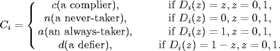
The key concept in methods for dealing with noncompliance is to divide the patient population into subpopulations according to their potential compliance behavior. For the ith patient, let Ci be the compliance behavior, which is defined as follows:
We observe the compliance behavior of a patient only partially, through the response to the actual treatment assignment the patient receives. If ![]() denotes the actual treatment assignment of the ith individual, we can observe
denotes the actual treatment assignment of the ith individual, we can observe ![]() , but we cannot observe the response to the alternative treatment assignment,
, but we cannot observe the response to the alternative treatment assignment, ![]() , where
, where ![]() . Let
. Let
Based on the compliance behavior, we can partition the population of patients into four subpopulations: ![]() ,
, ![]() ,
, ![]() , and
, and ![]() .
.
We define the ITT causal effect of Z on the outcome Y to be
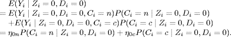
The population average ITT effect can be decomposed as
where
is called the average ITT effect of the treatment assignment (Z) on the outcome (Y) in the subpopulation of individuals whose compliance behavior types belong to ![]() .
.
Of the four subpopulation ITT effects, neither ITTn nor ITTa addresses causal effects of D (e.g., the receipt of flu shot) on Y because ITTn compares the outcomes of two groups that did not receive the treatment, and ITTa compares the outcomes of two groups that received the treatment. Only for the complier subpopulation and defier subpopulation, ITTc and ITTd compare the outcomes of those who received the treatment with the outcomes of those who did not receive the treatment.
From this discussion, we see that it is difficult to define causal effects of D on Y in the whole population without making additional assumptions. Hence, it may be more fruitful to assess causal effects of D on Y in the relevant subpopulations, the complier subpopulation and defier subpopulation. Since the existence of a defier group may not be realistic in practice, we focus on the subpopulation of compliers for the definition of the causal effects of D on Y. For the subpopulation of compliers, we define the average causal effect of D on Y as
called the complier average causal effect (CACE) (Imbens and Rubin, 1997a).
Next, we clarify information associated with each individual (Imbens and Rubin, 1997b). For the ith individual, we have defined five variables, Zi, Di(0), Di(1), Yi(0, Di(0)), and Yi(1, Di(1)), as well as the sixth variable Ci, which is a function of Di(1) and Di(0). Among the five variables, three variables are observable: the treatment assignment, ![]() ; the actual treatment received under the assigned treatment,
; the actual treatment received under the assigned treatment, ![]() ; and the observed outcome under the assigned treatment and actual treatment received,
; and the observed outcome under the assigned treatment and actual treatment received, ![]() . The other two variables are missing: the treatment the ith individual would have received under the alternative treatment assignment to the actual treatment assignment,
. The other two variables are missing: the treatment the ith individual would have received under the alternative treatment assignment to the actual treatment assignment, ![]() , where
, where ![]() ; the outcome the ith individual would have observed under the alternative treatment assignment and corresponding actual treatment received,
; the outcome the ith individual would have observed under the alternative treatment assignment and corresponding actual treatment received, ![]() . Of course, the sixth variable Ci is also missing.
. Of course, the sixth variable Ci is also missing.
To simplify the notation, for observed variables, we omit their subscripts. Hence, the observed data consist of (Zi, Di, Yi), where i = 1, ..., N; here, N is the sample size. Let ηzt = E(Yi(z, Di(z)) | Zi = z, Ci = t), ωt = P(Ci = t), and ξz = P(Zi = z), where z = 0, 1 and t = n, a, c, d. Without additional assumptions, these parameters are not identifiable, which means that different values of the parameters in the model can generate the probability distribution of the observed data. For a formal mathematical definition on model identifiability, see Lehmann and Casella (1998).
To make the model identifiable, we make three additional assumptions: strongly ignorable treatment assignment, monotonicity, and exclusion restriction. The strongly ignorable treatment assignment assumption is given as follows.
Note that a randomized trial satisfies this assumption.
The monotonicity assumption rules out the existence of defiers and is defined as follows.
In the flu shot example, the monotonicity assumption is plausible. It is unlikely physicians decide after receiving the reminder not to give flu shots to patients to whom they would have given a flu shot in the absence of the reminder. In general, for clinical trials with treatments that are believed to have some benefit, the monotonicity assumption is reasonable. Under the monotonicity assumption, ωd = 0. Hence, under the monotonicity assumption, the number of unknown parameters in the model is reduced by one.
The exclusion restriction assumption formalizes the notion that any effect of the treatment assignment on the outcome should be mediated by an effect of the treatment assignment on the actual treatment received. In the flu shot example, the exclusion restriction assumption means that any effect of the reminder on the outcome should be mediated by an effect of the reminder on the actual flu shot received. We only need to make the exclusion restriction assumption for never-takers and always-takers, formally defined as follows.
Under the exclusion restriction assumption, we have ηzt = ηt, t = n, a, and have reduced the number of unknown parameters by two. Under the above four assumptions, it can be shown that the CACE is estimable (Angrist et al., 1996). Next, we will discuss the four methods for making inferences about CACE, including the method of instrumental variables, the moment-based method, the maximum likelihood method, and the Bayesian method.
8.5 Method of Instrumental Variables
The method of instrumental variables is based on equation (8.2) and the exclusion assumption. From equation (8.2), we obtain
From the exclusion restriction, ITTn = ITTa = 0. Therefore,
From this expression, we see that to estimate CACE, we need to estimate ωc and ITT. Because of the strongly ignorable treatment assignment assumption and the exclusion restriction assumption, we have
From this formula, we obtain a moment-based estimator for ωn as follows:
Similarly, we obtain the following moment-based estimator for ωa:
Since ωc + ωa + ωn = 1, we obtain the moment-based estimator for ωc as follows:
We can estimate ITT by the following consistent estimator:
Therefore, the IV estimator for CACE is given as follows:
We can use the delta method to derive the asymptotic variance of ![]() as follows (Imbens and Rubin, 1997a):
as follows (Imbens and Rubin, 1997a):
Hence, we derive a variance estimator for the IV estimator as follows:
where

and

8.6 Moment-based Method
Since CACE = η1c − η0c, to estimate CACE, we need to estimate η0c and η1c. Under the monotonicity assumption, it is relatively easy to estimate ηn, ηa, and ωt (t = c, n, a) directly from the observed data.
We first show that ηzc (z = 0, 1) can be written as functions of ηn, ηa, and ωt as well as quantities that can be directly estimated from the observed data. Under the monotonicity assumption, we have Zi = 0 and Ci = c if and only if Di(0) = 0, Di(1) = 0 or Di(0) = 0, Di(1) = 1. Therefore,
Note that

Hence,
Or,
Similarly, we can obtain the following equation:
Or,
We observe that E(Yi | Zi = 0, Di = 1) and E(Yi | Zi = 1, Di = 1) can be estimated directly from the observed data. Therefore, to estimate η0c and η1c, we need to estimate ηn, ηa, and ωt (t = c, n, a). We next derive moment-based estimators for ηn and ηa. Note that Zi = 1 and Ci = n if and only if Zi = 1 and Di = 0 because of the monotonicity assumption. Hence, we have
Therefore, the moment-based estimator for ηn is
Similarly, we can obtain a moment-based estimator for ηa as follows:
We then derive moment-based estimators for ωt (t = c, n, a). Because of the strongly ignorable treatment assignment assumption, we have
From this formula, we obtain a moment-based estimator for ωn as follows:
Similarly, we obtain the following moment-based estimator for ωa:
Since ωc + ωa + ωn = 1, we obtain a moment-based estimator for ωc as follows:
Using (8.4) and (8.5), we derive moment estimators for η0c and η1c as follows:
and
Hence, the moment-based estimator for CACE is given as follows:
where ![]() and
and ![]() are defined by (8.6) and (8.7), respectively. Similar to derivation of the variance for the IV estimator in Section 8.5, we can also use the delta method to derive the asymptotic variance of
are defined by (8.6) and (8.7), respectively. Similar to derivation of the variance for the IV estimator in Section 8.5, we can also use the delta method to derive the asymptotic variance of ![]() .
.
8.7 Maximum Likelihood and Bayesian Methods
If we are willing to assume a distribution for Y, we can also derive maximum likelihood estimators for CACE. In this section, we assume that Y is binary and that (Z, D, Y) follows a multinomial distribution. The log-likelihood function of the observed data (Y, Z, D) can then be written as follows:
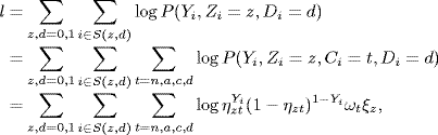
where S(z, d) = {i : Zi = z, Di = d}, which is determined by Zi = z and Ci = t. This likelihood can be further simplified by writing out the likelihood contributions of S(z, d).
- For i
 S(0, 0),

- For i S(0, 1),

- For i S(1, 0),

- For i S(1, 1),

Therefore, the log-likelihood function is given as follows:
Maximization of the above likelihood function would give us the ML estimate for θ = (ηtz, ωt, ξ).
Since the observed-data likelihood, given above, has a complicated form, involving a mixture structure over a large amount of missing data, directly maximizing the observed-data likelihood may present a computational challenge. To overcome this computational problem, we can use the expectation–maximization (EM) algorithm for computing the ML estimator ![]() for θ by treating Ci as missing data because the complete-data likelihood has a simple form if Ci were known for all patients.
for θ by treating Ci as missing data because the complete-data likelihood has a simple form if Ci were known for all patients.
The complete data would include Yi, Ci, Zi, and Di. The complete-data likelihood function is given by
Let ![]() , the number of subjects with Yi = y, Zi = z, and Ci = t, which is unobserved. We obtain the complete-data log-likelihood as follows:
, the number of subjects with Yi = y, Zi = z, and Ci = t, which is unobserved. We obtain the complete-data log-likelihood as follows:
The observed data consist of Y = (Y1, ..., YN), D = (D1, ..., DN), and Z = (Z1, ..., ZN).
As described in Chapter 4, the EM algorithm consists of iterations between E steps and M steps until convergence. In the (k + 1)th step of the E step, we take the expectation of the complete-data log-likelihood, given the observed data and the previous parameter estimate θ = θ(k) at tth step, E(lc(θ) | Y, D, θ = θ(k)). It is easy to show that

where

with d = Di(z).
The M step involves maximizing E(lc(θ) | Y, D, θ = θ(k)) with respect to θ, which gives us the following ML updated estimates:
and
We iterate between the E and M steps until ![]() converges, and the convergent value
converges, and the convergent value ![]() is the ML estimator of θ. The variance of the ML estimator can be obtained from the Fisher information matrix.
is the ML estimator of θ. The variance of the ML estimator can be obtained from the Fisher information matrix.
By assuming a prior distribution for θ, the Bayesian analysis makes inferences about θ, based on the posterior distribution of θ, which is defined as the conditional probability of θ, given the observed data. Since CACE is a function of θ, we can also compute the posterior distribution of CACE from the posterior distribution of θ.
It is worth noting that the analysis of a nonidentified model is less an issue with the Bayesian method as frequentist-based methods as long as a proper prior is used. This is because a proper prior always leads to a proper posterior distribution, even with a non-identified model for observed data. With a proper posterior distribution, all model parameters can be estimated using the posterior distribution (Eberly and Carlin, 2000). However, Gelfand and Sahu 1999) pointed out that priors that are too informative can dominate the inference and priors near to be improper would produce ill-behaved posteriors. Hence, a Bayesian method with a proper prior may be used to estimate CACE using fewer assumptions, for example, without assuming the exclusion restriction.
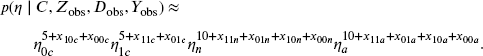
We use the data augmentation (DA) to find the posterior distribution of θ, given the observed data, p(θ | Zobs, Dobs, Yobs), because the complete-data likelihood function of (Zobs, Dobs, Yobs, C) has a much simpler form than the observed-data likelihood function.
Similar to the EM algorithm, we obtain the complete-data likelihood as follows:

DA requires three steps: (1) an initial draw from the prior for θ, (2) a draw from the complete-data posterior function, and (3) a draw from the conditional predictive distribution of Ci given Yi, Di, and Zi.
The posterior distribution can be sensitive to the choice of a prior distribution, because the observed-data likelihood has a mixture structure over a large amount of missing data.
We can choose a proper prior distribution with a simple conjugate form. The prior below corresponds to adding to the likelihood function 30 extra observations: there are 10 additional observations for each complier type; for each complier type, the 10 additional observations are split into 2.5 for each of the four combinations of the binary variables (Zi, Yi):
With prior independence of parameters, the complete-data posterior distribution of θ can be written as the product of five distributions: one for xi,
three for the compliance types,
and one for the outcomes,
8.8 Noncompliance and Missing Outcome Data
In practice, some clinical trials may also have missing outcomes for some subjects, in addition to noncompliance. Many methods have been proposed for dealing with both noncompliance and missing data. To get key ideas across, in this section, we introduce moment and maximum likelihood methods for estimating CACE under the latent ignorability assumption for the missing data mechanism when the outcome variable is binary in a randomized trial (Frangakis and Rubin, 1999; Zhou and Li, 2006).
To make a parameter identifiable, we need to make additional assumptions about the missing data mechanism. Here, we are making the latent ignorability assumption and the compound exclusion assumption proposed by Frangakis and Rubin 1999).
- Latent Ignorability: Potential outcomes and associated potential nonresponse indicators are independent within each level of the latent compliance covariate, that is,

- Compound Exclusion Restrictions for Never-Takers and Always-Takers: For never-takers and always-takers, Z influences Y and R only through D.
Here, the compound exclusion restriction for never-takers embodies the twin assumptions that within the subpopulation of never-takers, the distributions of the two potential outcomes P[Y(1, 0) = 1|Z = 1, D = 0] and P[Y(0, 0) = 1|Z = 0, D = 0] are identical, and that the distributions of the two missing data indicators P[R(1) = 1|Z = 1, D = 0] and P[R(0) = 1|Z = 0, D = 0] are also identical. In other words, the treatment assignment does not affect the outcome or missing data distributions for never-takers. The compound exclusion restriction for always-takers, similarly, comprises the twin assumptions that within the subpopulation of always-takers, the treatment assignment does not affect the outcome or missing data distributions.
To derive estimators for CACE, we need additional notations. Let γzt ≡ P[Ri = 1|Zi = z, Ci = t] be the probability of observing outcome Y for subjects with Zi = z and Ci = t. Let us define
the conditional probability of outcome Yi(z, Di(z)), given the complier type and the treatment assignment. We further define
the probability of complier type, given the observed treatment assignment and receipt.
Under the compound exclusion assumption, we have
Furthermore, under our assumptions, many of the conditional probabilities of complier types, given the observed data, are known:
Therefore, among ψzdt, only ψn00 and ψa11 are unknown parameters. To simplify notation, we denote the two parameters of interest: ψn00 = ψn and ψa11 = ψa.
The marginal distributions of potential outcomes and the missing data mechanism are defined by 10 parameters: ψn, ψa, ηn, ηa, η0c, η1c, γn, γa, γ0c, and γ1c. Let θ be a vector of these parameters; that is, θ = (ψn, ψa, ηn, ηa, η0c, η1c, γn, γa, γ0c, γ1c).
We first introduce some notation to describe data.
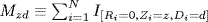
- Let
 , which represents the total number of subjects in the sample who have observed outcomes and who assigned to the treatment assignment z and who actually received the treatment assignment d.
 - Let
 , which is the total number of hospitalized subjects assigned to the treatment group z, receiving treatment d, and having the observed outcome.
 - Let
 , which is the total number of subjects in the sample who are missing the outcome and who assigned to the treatment assignment z and who actually received the treatment assignment d.
Next, we describe two estimation methods for θ: the moment-based method and the maximum likelihood method. We start with finding moment-based estimators for parameters in noncomplier subpopulations.
We first derive moment-based estimators for ψn and ψa. Under randomization, we expect P[Z = 0|C = n] = P[Z = 1|C = n]. Because never-takers, by definition, have Di = 0, we expect P[Z = 0, D = 0|C = n] = P[Z = 1, D = 0|C = n]. Hence, the expected number of never-takers with (Zi = 0, Di = 0) is the same as the number of never-takers with (Zi = 1, Di = 0). Similarly, the expected number of always-takers with (Zi = 1, Di = 1) is the same as the number of always-takers with (Zi = 0, Di = 1). Then, we obtain that
and
Therefore, the moment-based estimators for ψn and ψa are given as follows:
We next derive the moment-based estimators for ηn, ηa, γn, and γa. By the latent ignorability assumption, we have P[Y = 1|Z = 1, C = n] = P[Y = 1|Z = 1, C = n, R = 1] and P[Y = 1|Z = 0, C = a] = P[Y = 1|Z = 0, C = a, R = 1]. Hence, we have
and
It follows that the moment-based estimators for ηn and ηa are given by
respectively.
Using the compound exclusion assumption, we have the following results:
and
Hence, the moment-based estimators for γn and γa are given by
respectively.
We then derive moment-based estimators for parameters in complier sub-populations. We first observe that we can express the directly estimable quantity P(R = 1 | Z = z, D = d) as mixtures of parameters of the noncomplier population, γzt and ψzdt, as well as the ratio of P(R = 1, Z = z, D = πzd) and P(Z = z, D = ξzd). That is,

By taking z = 0 and 1 in the above expression, we obtain
Solving γ0c and γ1c in (8.8), we obtain
and
Since
are unbiased estimators of πzd and ξzd, respectively, the moment-based estimators for γ0c and γ1c are
and
respectively, where
and
Using the same idea as before, we express parameters for the complier population, η0c and η1c, as a function of estimable quantities. We can show that
By simple calculation, we can show that
and
Therefore,
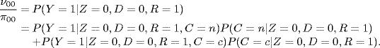
Similar to the expression for ν00/π00, we obtain
By solving for η0c and η1c in the above equations, we obtain
and
Hence, we obtain the following moment-based estimators for η0c and η1c:

Using the above results, we can also estimate the proportions of the three complier types, ωn, ωa, and ωc, as follows:
where N is the total number of subjects in the sample. The resulting estimator for the local CACE is given as
We apply the bootstrap method to compute the standard errors for the moment estimators.
One potential problem with the moment estimators is that they are not constrained to the range of the parameters they estimate. Next, we develop maximum likelihood estimators for estimating causal parameters.
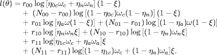
It can be shown by simple calculation that the observed-data log-likelihood l(θ) ≡ log L(θ) is given by

To obtain the maximum likelihood estimator ![]() for θ, we can directly solve the score function of θ, which is the partial derivative of the log-likelihood with respect to θ, S(θ) = ∂ l(θ)/∂ θ. Using the Fisher information matrix, we obtain standard error estimates for these parameters.
for θ, we can directly solve the score function of θ, which is the partial derivative of the log-likelihood with respect to θ, S(θ) = ∂ l(θ)/∂ θ. Using the Fisher information matrix, we obtain standard error estimates for these parameters.
The above direct ML estimation, based on the observed data, has one major drawback: the observed-data likelihood, given in equation (8.9), has a complicated form, involving a mixture structure over a large amount of missing data. To overcome this drawback, we propose to use the EM algorithm for computing the ML estimator ![]() for θ by treating Ci as missing data because the conditional complete-data likelihood has a simple form if Ci were known for all patients.
for θ by treating Ci as missing data because the conditional complete-data likelihood has a simple form if Ci were known for all patients.
In the E step of the EM algorithm, we compute the conditional expectation of the complete-data likelihood function, given the previous parameter estimate, denoted by θ(k), and the observed data. In the M step, we maximize this expectation with respect to θ, typically by differentiation, to obtain the new parameter estimate θ(k+1). We repeat the E and M steps until the process converges at step K, where ![]() . Here,
. Here, ![]() is a very small constant. The one major advantage of using the EM algorithm here is that the EM algorithm yields an explicit solution for θ(k+1) in terms of θ(k) and the observed data, which simplifies computation. Next, we give the details on the E and M steps.
is a very small constant. The one major advantage of using the EM algorithm here is that the EM algorithm yields an explicit solution for θ(k+1) in terms of θ(k) and the observed data, which simplifies computation. Next, we give the details on the E and M steps.
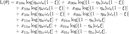
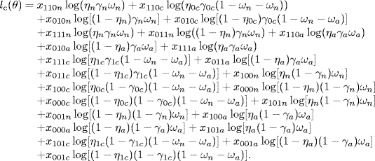
Let xyrzt be the number of subjects with Yi = y, Ri = r, Zi = z, and Ci = t, 1 ≤ i ≤ N. Then, we obtain the following complete-data log-likelihood:
In the E step, we take the expectation of the complete-data log-likelihood, given the observed data and the previous parameter estimate θ = θ(k), and obtain the following results:
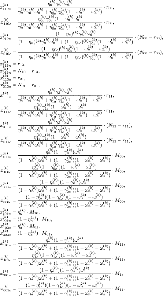
In the M step, we find the next iteration estimate θ(k+1) by finding the roots of the partial derivatives of E[lc(θ)|Y, D, Z, θ = θ(k))] with respect to θ,
where Yobs = (R1Y1, ..., RNYN) = (Y1, ..., Yn), D = (D1, ..., Dn), and Z = (Z1, ..., Zn) are observed data. We can show that Sc(θ) has the following elements:
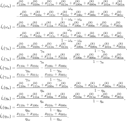
Solving the above functions would give us the estimates of ![]() ,
, ![]() ,
, ![]() ,
, ![]() ,
, ![]() ,
, ![]() ,
, ![]() ,
, ![]() ,
, ![]() , and
, and ![]() . We can also obtain
. We can also obtain ![]() and
and ![]() by noting that ψn = ωn/(1 − ωa) and ψa = ωa/(1 − ωn).
by noting that ψn = ωn/(1 − ωa) and ψa = ωa/(1 − ωn).
8.9 Analysis of the Two Examples
We illustrate the methods introduced in the previous sections with the two examples, described in Section 8.2.
8.9.1 Analysis of Vitamin A Supplement Example
Returning to the vitamin A supplement example, we are interested in estimating the causal effect of taking the vitamin A supplement on mortality. Since the mortality rate for children who were assigned the intervention but did not take the vitamin A supplement is 0.014, much higher than the mortality rate of control children, 0.006, it seems like intervention children who did not take vitamin A supplement are more sick than the control children who also did not take vitamin A supplement. Hence, the per-protocol analysis, which discard all intervention children who did not take vitamin A supplement, would produce a biased estimate of the effect of taking vitamin A supplement versus not taking vitamin A supplement because the intervention group of children was healthier than the control group.
To obtain unbiased estimates, we need to use IV methods. In this example, since no subjects from the control group receive vitamin A supplements, we have Di(0) = 0, but Di(1) = 0 or 1, where Di denotes the receipt of vitamin A supplement for subject i. Hence, monotonicity holds, and ωa = ωd = 0. The estimated IV estimate is 0.0032 with a 90% confidence interval of (0.0009, 0.0055) (Imbens and Rubin, 2014).
Applying the ML and Bayesian methods to this data set under the exclusion restriction assumption, we obtain the MLE for CACE as 0.0032 with the 90% confidence interval of (0.0012, 0.0051). The mean of posterior mean under the exclusion is 0.0031 and 90% posterior confidence interval is (0.0012, 0.0051) (Imbens and Rubin, 2014).
8.9.2 Flu Shot Example
In the flu shot example, described in Section 8.2.2, we have the problem of both missing data and noncompliance. We apply the moment-based and ML methods, which were introduced in Section 8.8 and can handle the problem of both missing data and noncompliance.
With the ML method, we obtain the estimated CACE of −0.009 with a standard error of 0.112. With the moment method, we obtain the estimated CACE of 0.009 with a standard error of 0.479. The corresponding 95% confidence intervals for CACE using the ML and moment methods are (− 0.211, 0.229) and (− 0.948, 0.930), respectively.
Although the moment and ML estimates of CACE are different, both give the same conclusion that influenza vaccination is not associated with reduced risk of hospitalization for respiratory illness.
8.10 Other Methods for Dealing with both Noncompliance and Missing Data
In the previous section, we introduced the moment-based and ML methods for dealing with the problem of both noncompliance and missing data. There are other methods available for dealing with this problem. Taylor and Zhou (2009b) further extended the results of Zhou and Li (2006) by developing the asymptotic theory for their moment estimator and proposed a method to assess sensitivity of the moment method for violation of the assumption of latent ignorability.
Taylor and Zhou (2009a) have also developed the multiple imputation (MI) method for CACE. As discussed in the previous chapters, the MI method has several advantages over the ML methods. An important advantage of the MI analysis (and the Bayesian analysis) over and above the likelihood methods is that neither the monotonicity nor the compound exclusion restriction, which have been used to develop and justify estimation procedures, is essential, and violations of these assumptions can be addressed. However, for both Bayesian and MI methods, identification is based entirely on a carefully thought-out (or mathematically tractable) prior distribution.
MI has statistical properties that closely match the optimality of maximum likelihood methods (although not exactly optimal since ML involves no simulation), with the principal advantage being that it can be used in almost any situation, whereas ML is much more restricted in its applications, perhaps requiring specially designed EM algorithms and sometimes difficult analytic or numerical integration on the log-likelihood for interval estimates.
Another important advantage of the MI analysis over the Bayesian and ML methods is that MI works in conjunction with standard complete-data methods and software so that after the imputations are generated, data analysts who are not professional statisticians can apply standard complete-case analysis to the multiply imputed data sets. And since the imputation phase is operationally distinct from subsequent analysis, given a set of m imputations, many different analyses can be performed, making it unnecessary to reimpute when a new analysis is considered. By using a Bayesian framework for imputation and a frequentist approach to examining the estimator, one is also able to take advantage of the Bayesian framework, for example, by relaxing certain assumptions while having the ability to make direct comparisons with other frequentist methods. MI is especially promising when standard complete-case analysis is difficult to modify analytically in the presence of missing data, as in the case of nonignorable missing data or multivariate outcomes.
The above-discussed methods may still yield biased estimators of the CACE if the missing data mechanism is a different type of not missing at random (NMAR) from latent ignorability. Often, the mechanism of missing outcome Y can depend on missing values of Y. For example, some subjects may drop out of a study because of patient's worsening condition, Y; that is, the outcome Y has a direct effect on the missing data mechanism, which is called completely nonignorable missing data.
Chen et al. 2009) showed that, under certain conditions, the parameters of interest were identifiable even under completely nonignorable missing data. They then derived their maximum likelihood and moment estimators and evaluated their finite sample properties in simulation studies in terms of bias, efficiency, and robustness. Their simulation studies show that the proposed estimators behave reasonably well for finite sample sizes.
Appendix 8.A: Multivariate Delta Method
The delta method is a powerful tool for deriving asymptotic distribution of a function of vector of random variables. Suppose that X1, X2, ... are a sequence of some k-dimensional random vectors, which satisfy the following condition:
where Y is some k-dimensional random vector. Also, suppose that g is a mapping from ![]() to
to ![]() with the finite first derivative with respect to a, ∂g(a)/∂ a, with
with the finite first derivative with respect to a, ∂g(a)/∂ a, with ![]() . Then, the multivariate delta method states the following result:
. Then, the multivariate delta method states the following result:
A proof of this result can be obtained by using the first-order multivariate Taylor expansion (DasGupta, 2008; Vaart, 2000).