
CHAPTER 9
Analysis of Equity Risk Using Fundamentals Factor Models
Throughout this book, we have described various measures computed from financial statements and ratios that have combined financial statement data and market data. We discussed how these measures can be used to evaluate the economic prospects of a company. In Chapter 5, we began the process of showing how a company's stock can be valued using a discounted value approach and we presented several dividend discount models that are used by practitioners. In this chapter, we look at another approach to valuation, factor models. While there are different types of factor models, our focus in this chapter is on fundamental factor models, which use the various measures discussed in this book as inputs to the model.
Our objective is not to discuss how factor models are built. Rather, our objective is simply to demonstrate how various measures are used in models to estimate the expected return on stocks and to manage portfolios.
MEASURING RISK
It is well known that there is a positive relationship between risk and expected return. That is, the greater the risk, the higher the expected return that investors want. This is a basic principle of financial theory. The tough part is figuring out the appropriate way to define risk and to how to quantify that risk.
The term “risk” is used very casually in the financial press and in day-to-day conversations about investments. Financial theory provides a more specific definition of risk. There are several models in financial theory that define risk quantitatively and relate that risk to the expected return. We refer to these models as asset pricing models.
Total Risk
The first major step in the development of asset pricing models was to show how to think about and quantify risk in general. Harry Markowitz explained that the risk of an individual stock should be quantified by using the standard deviation or variance of possible returns.1
Specifically, we can measure risk by the standard deviation or variance of the stock's anticipated returns. This measure of risk is referred to as total risk and we will see why it bears this label shortly. Thus, according to financial theory, the total risk that an investor faces from investing in a stock is the standard deviation or variance of a stock's return.
Consider a simple example. Suppose a stock has the following possible returns, with a probability (or likelihood) associated with each one:
| Scenario | Probability | Possible Return |
| Boom market | 30% | 15% |
| Normal market | 50% | 8% |
| Bust market | 20% | −2% |
The expected return is the weighted average of the possible returns, where each return is weighted by its probability of occurrence. The expected return is 8.1%. The more challenging part of the calculations is to determine the variance and standard deviation of this distribution. Like a standard deviation for a sample, we consider that each possible return deviates from the expected return. The next step is to weight these squared deviations by the probabilities; the sum of the weighted squared deviations is the variance. The square root of the variance is the standard deviation of the possible returns. We provide the general steps in this calculation in Exhibit 9.1 and detail these calculations for our example in Exhibit 9.2.
EXHIBIT 9.1 Process for Calculating a Standard Deviation of Possible Returns
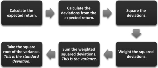
EXHIBIT 9.2 Calculation of the Expected Return and Standard Deviation of Returns
The calculation of the standard deviation of the possible returns, though helpful in understanding how investors may use expectations in pricing, is not realistic of what investors or analysts actually do. A more practical approach to estimating a standard deviation is calculating historical returns and using the distribution of these returns as an estimate of the standard deviation of future returns. Of course, when using this approach we are assuming that the variability of stock prices in the past is representative of the volatility of stock prices in the future.
Consider the returns of Apple, Inc. Using sample statistics, we can calculate the mean monthly return and the standard deviation.2 We start with month-end stock prices and then calculate each month's returns. Because the mean and standard deviation will be different for different periods, the investor or analyst must apply judgment and care in forecasting the mean and dispersion of returns based on historical returns:
| Period | Mean | Standard Deviation |
| 1987-2011 | 2.50% | 13.90% |
| 1992-2011 | 2.44% | 13.92% |
| 2002-2011 | 3.67% | 11.05% |
| 2007-2011 | 3.23% | 10.67% |
The standard deviation is a measure of the dispersion of the possible returns: the greater the dispersion, the greater the risk. Therefore, the larger the standard deviation of an asset's returns, the greater the asset's total risk.
Markowitz shows that the total risk of a portfolio of stocks is not found by simply adding up the total risk of the individual stocks included in the portfolio. Rather, the total risk of a portfolio, as measured by the variance of the portfolio's return, depends on the correlation (or covariance) between each pair of assets in the portfolio.
A key element of Markowitz's demonstration is that the lower the correlation, the lower the total risk of the portfolio. The procedure for diversification is then to combine stocks in a portfolio, giving recognition to the correlation between assets.
Markowitz then went on to show how an efficient portfolio can be created. An efficient portfolio is a portfolio where for a given level of expected return, the portfolio's total risk will be the smallest of all possible portfolios that can be created.
Systematic Risks and Unsystematic Risk
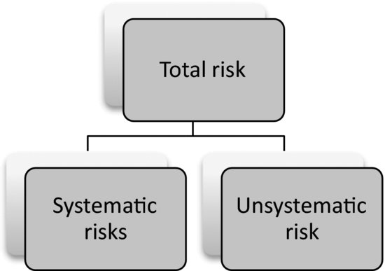
Subsequent analysis of risk developed two principles. The first is that in a reasonably efficient stock market, investors are only rewarded for accepting risks that cannot be diversified away by an investor. The second principle is that total risk, as measured by the variance of an asset's return, can be decomposed into two general categories of risk—risks that can be diversified away and risk that cannot be diversified away.
We refer to the risks that an investor cannot diversify away as nondiversifiable risk or systematic risk. We refer to any remaining risk as unsystematic risk or residual risk. We diagram this decomposition in Exhibit 9.3. Investors should be compensated for the systematic risks but not for unsystematic risk.
EXHIBIT 9.3 Risk Composition
ASSET PRICING MODEL
There are asset pricing models in financial theory that define risk quantitatively and relate that risk to the expected return.
Key to these models is identifying systematic risks. We refer to such risks as factors or risk factors. Asset pricing models show the relationship between the expected return for an asset and risk factors. The two dominant asset pricing models are the capital asset pricing model and the arbitrage pricing theory model.
Capital Asset Pricing Model
Let's look at a popular asset pricing model, the capital asset pricing model (CAPM). Based on certain assumptions, CAPM says that there is only one form of systematic risk. This systematic risk is the movement of the market in general. Mathematically, we can express the return based on the CAPM as the sum of the risk-free rate of return, Rf, and the premium for bearing market risk, βi [E(Rm – Rf)]:
![]()
| where | Rm is the expected return on the market index. |
| βi is the measure of systematic risk for asset i. |
In theory, the market is defined as all assets. However, in practice, in the application of the CAPM to stocks, the market is defined as a broad-based equity market index such as the Standard & Poor's 500.
The βi is the stock's beta. Mathematically, it is the ratio of the covariance of the stock's return with the market to the total risk (variance) of the market. It is a measure of systematic risk because it quantifies how the stock's return systematically varies with the market's return. The CAPM asserts that the expected (or required) return on an individual asset is a positive, linear function of its index of systematic risk as measured by beta. The higher the beta, the higher the expected return. Notice that it is only an asset's beta that determines its expected return—which is what we noted earlier that the CAPM assumes only one form of systematic risk.
There are two approaches used to estimate beta. The first is to use a time series of monthly or weekly returns to estimate the following relationship between the return on the stock and the return on the market:
![]()
| where | Ri is the observed return for period t for stock i. |
| Rmt is the observed return on the market index for period t. | |
| Bi is the slope for stock i which we refer to as the historical beta. |
This regression equation that we use to obtain the estimate for beta for the CAPM is the market model. The intercept (α) and slope (β) are the parameters to be estimated and the latter is the estimate used for the beta of stock i in the CAPM.
The problem with using historical beta is that beta captures fundamental attributes of a company such as leverage, size, earnings growth, and liquidity, and these attributes change over time. What is important is that the analyst use the future beta in estimating the expected return when employing the CAPM. Because company attributes change, historical beta may not be a good predictor of future beta.
This problem leads to the second approach to estimating beta. The approach involves first calculating historical beta for all firms using the market model. Suppose there are N firms and therefore N estimated betas denoted by i. Then suppose that there are k fundamental attributes that have been found to affect the beta of firms. We will denote these attributes at a given point in time as X. Then we estimate the following cross-sectional multiple regression:
![]()
where the α ‘s are the parameters to be estimated and the Xk,i is the observed fundamental attribute k for firm i.3
Given the estimates for the parameters, we estimate a company's beta by substituting its fundamental attributes into the previous equation. The resulting estimated beta is a fundamental beta.4
The assumption in using this procedure is that for all companies the fundamental beta is affected in the same way for each fundamental attribute. For example, it assumes that an increase in the leverage ratio by a certain amount affects the fundamental beta of Microsoft in the same way it affects Kmart.
Consider an application of this to the analysis of a single company. Suppose we have the estimates for the coefficients in the fundamental beta equation. If the company we are analyzing is acquiring another company and its liquidity returns, leverage, and other fundamental factors are expected to change, the analyst can use this equation and the estimated coefficients to estimate the company's new beta.
The research into the fundamental factors of beta indicates that operating leverage and financial leverage are drivers of a company's systematic risk.5 In addition, researchers have found that companies in industries that are more cyclical have higher betas.6 In their analysis of the drivers of betas of value and growth stocks, John Campbell, Christopher Polk and Tupmo Vuolteenaho find that betas are driven, in large part, by the cash flow characteristics of the companies.7
Arbitrage Pricing Theory Model
In 1976, Stephen Ross developed an alternative equilibrium asset pricing model He derived this model based purely on arbitrage arguments, and hence he called it the arbitrage pricing theory (APT) model.8 In its simplest form, arbitrage is the simultaneous buying and selling of a security at two different prices in two different markets. The arbitrageur profits without risk by buying cheap in one market and simultaneously selling at the higher price in the other market.
In the APT model there may be more than one systematic risk, whereas the CAPM asserts that there is only one systematic risk. Further, unlike the CAPM, the APT model does not specify the identity of the factors—just that they may exist.
Using the APT model, we can specify the return on asset i in terms of the returns on the risk-free rate of interest and the returns on the excess returns associated with the K factors:
![]()
| where | βi,Fj is the sensitivity of asset i to the j-th factor, and |
| [E(RFj) – Rf] is the excess return of the j –th sensitivity factor over the risk-free rate. |
We can think of the excess return as being the risk premium associated with the j-th systematic risk.
The APT model states that investors want to be compensated for all the factors that systematically affect the return of a stock. The compensation is the sum of the products of the each factor's systematic risk (βi,Fh), and the risk premium assigned to it by the market [E(RFh − RF)]. As in the case of the CAPM, an investor is not compensated for accepting unsystematic risk. Examining the APT and CAPM, we can see that if the only factor in the APT is market risk, the APT model reduces to the CAPM.
Supporters of the APT model argue that it has several major advantages over the CAPM. First, it makes less restrictive assumptions about investor preferences toward risk and return. Second, no assumptions are made about the distribution of security returns.
FACTOR MODELS
CAPM and APT are equilibrium models that tell us the relationship between risk and expected return. In practice, there are three types of factor models that seek to identify a parsimonious set of factors that explain stock returns: statistical factor models, macroeconomic factor models, and fundamental factor models. We briefly describe the first two models below and then provide more detail on the model of principal interest to us, fundamental factor models. The key in the application of factor models to equity valuation is identifying the risk factors.
In a statistical factor model, historical and cross-sectional data on stock returns are tossed into a statistical model. Using a statistical technique, principal components analysis, “factors” are derived that best explain the variance of the observed stock returns. For example, suppose you start with the monthly returns for 3,000 companies for 10 years. The goal of principal components analysis is to produce “factors” that best explain the observed stock returns. Let's suppose that there are six “factors” that do this. These “factors” are statistical artifacts and referred to as latent factors. The objective in a statistical factor model is to determine the economic meaning of each of these statistically derived factors.
Because of the problem of interpretation, it is difficult to use the factors from a statistical factor model for valuation and risk control. Instead, practitioners prefer the two other models that allow them to pre-specify meaningful factors, and thus produce a more intuitive model. In a macroeconomic factor model, the inputs to the model are historical stock returns and observable macroeconomic variables. These variables are raw descriptors or simply descriptors. The goal is to determine the macroeconomic variables that are pervasive in explaining historical stock returns; those variables are the factors and we include them in the model. We estimate the responsiveness of a stock's return to these factors using historical time series data.
FUNDAMENTAL FACTOR MODELS
Fundamental factor models use company and industry attributes and market data as the basic inputs to the model. Examples of the basic inputs are price/earnings ratios, book/price ratios, earnings momentum, and financial burden measures. The fundamental factor model uses stock returns and the basic inputs about a company and tries to identify which basic inputs are important in explaining stock returns. Those basic inputs about a company that are found to be important in explaining stock returns comprise a fundamental factor model. In practice, an investor can either develop a fundamental factor model or purchase one from a commercial vendor.
Commercial vendors of fundamental factor models include:
- MSCI Barra
- Axioma
- APT
- Northfield
- RSquared
We discuss the MSCI Barra fundamental factor model next and then describe a popular model developed by Eugene Fama and Kenneth French, referred to as the three-factor model.
MSCI Barra Fundamental Factor Model
In the MSCI Barra fundamental factor model, there are eight risk indexes that are specific to the stock:
We provide definitions of the risk indices and related descriptors in Exhibit 9.4. Three of the risk indexes include at least one of the measures of earnings, earnings forecast, or price-to-earnings ratio—the growth risk index, the earnings yield risk index, and the earnings variability risk index. The growth index and the dividend yield risk index have raw descriptors using one of the dividend measures.
EXHIBIT 9.4 Sample Fundamental Data Used in MSCI Barra Models
These risk factors are obtained from data from both a firm's financial statements and equity market information. In Exhibit 9.5 we show sample fundamental data used in the model. As you can see in this exhibit, several of these descriptors are financial ratios that we have discussed in Chapter 4 as well as other measures taken or constructed from the financial statements.
EXHIBIT 9.5 MSCI Barra Global Equity Model (GEM2)
| Risk Indexes | Description | Descriptors |
| Momentum | This risk index captures common variation in returns related to recent stock price behavior. | Historical α from the market model Relative strength, 6 months Relative strength, 12 months |
| Volatility | This risk index captures relative volatility using measures of both long-term historical volatility and near-term volatility. | Historical beta Daily standard deviation of returns Cumulative range of returns over time Historical standard deviation of the error in the market model |
| Size | This risk index captures differences in stock returns due to differences in the market capitalization of companies. | Log of market capitalization |
| Size nonlinearity | This risk index captures deviations from linearity in the relationship between returns and log of market capitalization. | Cube of the log of market capitalization |
| Growth | This risk index uses historical growth and profitability measures to predict future earnings growth.a | Long-term predicted earnings growth Sales growth, five year Earnings growth, five year |
| Liquidity | This risk index relates to the relative trading activity of the stock.a | Average share turnover, previous 12 months Average share turnover, previous 3 months Share turnover, previous one month |
| Value | This risk index distinguishes between value stocks and growth stocks using the ratio of book value of equity to market capitalization.a | Forward earnings to price ratio Book to price ratio Cash earnings to price ratio Trailing earnings to price ratio Dividend to price ratio |
| Leverage | This risk index measures the financial leverage of a company.a | Market leverage (i.e., market value of invested capital to market capitalization) Book leverage (i.e., book value invested capital to book value of equity) Debt-to-assets |
| aStandardized on a country-relative basis. Source: Jose Menchero, Andrei Morozov and Peter Shepard, “The Barra Global Equity Model (GEM2),” Research Notes, September 2008, MSCI Barra. |
||
Fama-French Three-Factor Model
Now let's look at the factor models suggested by Eugene Fama and Kenneth French in their 1992 and 1993 studies.10 They examine the relationship between stock returns, beta, and several fundamental factors, including the earnings-price ratio, leverage, size, and book-to-market value of equity. They observe that, in addition to the market index, stock returns can be explained by size (that is, market capitalization) and the book-to-market equity ratio. For example, in their three-factor model, Fama and French present factors that are comparisons of returns:
| SMB: Small minus big | Average return for the three smallest portfolios, less the average return on the three largest portfolios. |
| HML: High minus low | Average return on the two value portfolios (that is, stocks with high book-to-market ratios), less the average return on the two growth portfolios (that is, stocks with low book-to-market ratios). |
| RM – Rf | Return on the market, less the return on a risk-free security |
In general, smaller capitalization firms have greater returns than larger capitalization firms. Further, firms with high book-to-market ratios have higher returns than firms with lower book-to-market ratios. Notice that the market index is still a factor in the Fama-French model. The difference between their model and the CAPM (an equilibrium model) is due to the presence of the book-to-market and capitalization in their model.
Applications of Fundamental Factor Models
The output of a fundamental factor model is the expected return for a stock after adjusting for all of the risk factors. This return is the expected excess return. From the expected excess return for each stock, we can compute an expected excess return for a portfolio comprised of stocks. This is the weighted average of the expected excess return for each stock in the portfolio. The weights are the percentage of a stock's value in the portfolio relative to the market value of the portfolio. Similarly, a portfolio's sensitivity to a given factor risk is a weighted average of the factor sensitivity of the stocks in the portfolio.
The set of factor sensitivities is then the portfolio's risk exposure profile. Consequently, the expected excess return and the risk exposure profile can be obtained from the stocks comprising the portfolio. Since a stock market index or benchmark is nothing more than a portfolio that includes the universe of stocks making up the index, an expected excess return and risk exposure profile can be determined for an index. This allows a manager to compare the expected excess return and the risk profile of a stock and/or a portfolio to that of a market index whose performance the portfolio manager is measured against.
Portfolios can be constructed by managers so as to have the desired exposure to fundamental factors and, hence, risk. To understand what this means, it is necessary to understand what the manager is attempting to do. A client specifies a benchmark for a manager. The goal of the manager is to outperform the benchmark. A common benchmark is the S&P 500. The benchmark has the risk exposures as defined by the fundamental factor model. The distinction between active portfolio management and passive portfolio management is that the latter tries to match the performance of the benchmark while the former seeks to outperform the benchmark.
In terms of fundamental factor models, a portfolio manager who follows a passive strategy known as indexing will seek to construct a portfolio to match the factor exposures of the benchmark. Of course, the manager can do this by buying all the stocks in the benchmark. Alternatively, the manager can use an optimization program to construct a portfolio whose exposure to the factors is such that the portfolio constructed has minimal risk of not matching the performance of the benchmark. That is, the constructed portfolio has minimal “tracking error.”
Active portfolio management requires that the manager make active bets. In terms of fundamental factor models, the bets are in the form of departures of the constructed portfolios exposure to the factors from the exposure of the factors in the benchmark.
SUMMARY
We can measure the total risk of a stock by the variance or standard deviation of the stock's return. The risk of a portfolio, however, depends on the correlation of returns of the stocks in the portfolio.
We can divide the total risk of a stock into systematic risk and unsystematic risk. Investors should be rewarded, in terms of a higher return, only for accepting systematic risks.
An asset pricing model shows the relationship between the systematic risks and expected return. The key is to determine the systematic risks. The capital asset pricing model asserts that there is only one systematic risk, whereas the arbitrage pricing model allows for more than one systematic risk.
Factor models assume that there may be more than one systematic risk. There are three types of factor models: statistical factor models, macroeconomic factor models, and fundamental factor models. The factors in a statistical factor model are statistical artifacts and are therefore difficult to interpret, and such models are rarely used by practitioners. The more common factor models are the macroeconomic factor model and the fundamental factor model. The raw descriptors in a macroeconomic factor model are macroeconomic variables; in a fundamental factor model the raw descriptors are fundamental variables for a company. In a factor model, the sensitivity of a stock's return to a factor is estimated.
The risk exposure profile of a stock is identified by the set of factor sensitivities. The risk exposure profile of a portfolio is the weighted average of the risk exposure profile of the stocks in the portfolio. The power of a factor model is that given the risk factors and the factor sensitivities, a portfolio's risk exposure profile can be quantified and controlled.
REVIEW
1. Harry M. Markowitz, “Portfolio Selection,” Journal of Finance 7, no. 1 (1952): 77–91.
2. The mean and standard deviation calculations for a sample of returns are calculated in a manner similar to the expected return and standard deviation, but in the case of the sample statistic each observation is weighted equally instead of being weighted by a probability. We calculate the monthly returns using the month end stock prices of Apple Inc. from finance.yahoo.com.
3. The estimated α's provide information on the change in β for a given one unit change in XK.
4. The term fundamental beta was first coined by Barr Rosenberg and Vinay Marthe in “The Prediction of Investment Risk Systematic and Residual Risk,'' Proceedings of the Seminar of the Analysis of Security Prices, University of Chicago, November 1975: 85-225.
5. See, for example, Baruch Lev, “On the Association Between Operating and Risk,'' Journal of Financial and Quantitative Analysis 9, no. 4 (1974): 627-642; and Stewart Myers, “The Relationship Between Real and Financial Measures of Risk and Return,'' in Risk and Return in Finance, Irwin Friend and James Bicksler (eds.), Cambridge, MA: Ballinger, 1977).
6. Myers, “The Relationship Between Real and Financial Measures of Risk and Return,'' 1977.
7. John Y. Campbell, Christopher Polk and Tuomo Vuolteenaho, “Growth or Glamour? Fundamentals and Systematic Risk in Stock Returns,'' Review of Financial Studies, 23 (2008): 305-344. In their analysis, they break betas into two parts: that which is driven by changes in cash flow estimates and that which is driven by discount rate changes. The authors explain the differences in betas for value and growth stocks with these drivers. For example, they find that growth stock's higher betas are attributed to the higher cash-flow uncertainty of these companies.
8. Stephen Ross, “The Arbitrage Theory of Capital Asset Pricing,'' Journal of Economic Theory 13 (1976): 341-60, and Stephen Ross, “Risk, Return and Arbitrage,'' Risk Return in Finance ed. I. Friend and J. Bicksler, Cambridge, Mass.: Ballinger (1976).
9. The firm updates its fundamental factor model periodically.
10. Eugene F. Fama and Kenneth R. French, “The Cross-Section of Expected Stock Returns,'' Journal of Finance 47, no. 2 (1992): 427-465, and Eugene F. Fama and Kenneth R. French, “Common Risk Factors in the Returns on Stocks and Bonds,'' Journal of Financial Economics 33, no. 1 (1993): 3-56.