
12. Tools and Procedures
,Our two purposes in this chapter are (1) to provide you with a handy tool for assessing risks and (2) to give you some grounding in how to make use of it. The tool, called RISKOLOGY, is freely downloadable from our Website (http://www.systemsguild.com/riskology). It’s a risk model in the sense described in the previous chapter. The tool is meant to be used in conjunction with your own production model or parametric estimator. Our tool will not estimate how long your project will take; all it will do is tell you how much uncertainty ought to be associated with whatever estimate you come up with.
The model is presented in the form of a spreadsheet. It comes with the logic needed to work with a set of quantified risks, as well as a starter database for four of the core risks of software development. (We discuss the core risks in Chapter 13.)
Just as you can drive a car without understanding all the intricacies of its motor and control systems, so too can you use the risk model without an insider’s knowledge of how it works. In this chapter, though, we’ll give you a peek inside the model. This will serve to demystify it a bit, and to give you a leg up if you decide to customize the spreadsheet to better match your own circumstances. Customization may be important because it enables you to eliminate at least some of the apparent uncertainty about your projects. Your locally collected data may be more optimistic and also more applicable than our industry-wide data.
Before we launch into the details, here’s a promise to set your mind at ease: We haven’t put any hairy mathematics into this chapter. If you can handle a bit of arithmetic, the chapter should be accessible to you. If you are up to using a spreadsheet to forecast your retirement income, for example, you shouldn’t have any trouble taking the risk model apart and putting it back together, in case you decide to customize it.
Complex Mixing
At the heart of any risk model is a technique for determining the combined effect of two or more uncertainties:
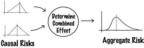
Toward the end of the next chapter, we’ll show how this works for software projects. Right here, though, we’re going to demonstrate the concept on an admittedly contrived problem that’s a bit easier to grasp.
Let’s say that you’re a runner. You jog every day, faithfully, but vary the time depending on your other commitments. Your daily workout takes anywhere from fifteen minutes to nearly an hour. You keep records and find that, fairly independent of distance (within this time range), your running speed varies from six-and-a-half to nine miles an hour. You’ve done this for so long that you have a respectable record:

The actual data was probably in the form of a bar chart; what we’ve shown here is the envelope curve that approximates that bar chart. This looks like an uncertainty diagram, and that’s exactly what it is. In fact, it can be presented in the two usual forms, as shown below:

This distribution of past results can be seen as a representation of uncertainty about how fast you’ll run the next time out.
Suppose your speed is not the only uncertainty affecting your next run. Suppose you’ve decided to run around a path of unknown length: the perimeter of a golf course. Since you’ve never run there before, you’re not at all sure just how long a run it will be. You do have some data, however, from the Professional Golfers’ Association, about course perimeters, telling you that the distance around the courses varies from two to four miles, with the most likely perimeter at approximately 2.8 miles. This, too, can be expressed as a distribution:

The data here is more granular, due to the paucity of data points.
Now, how long will your next run take you? You remember that time is distance divided by rate (miles run divided by miles per hour of speed). If the distance and the speed were fixed numbers, you could do the arithmetic, but in this case, both parameters are uncertain, expected to vary over a range. This assures that there will be some uncertainty in the result, as well:

In order to derive the output curve that is the composite of the two input curves, we would need to adopt a method from integral calculus. But such hairy mathematics is not allowed in this chapter. So, what can we do?
Instead of deriving the curve, we’re going to approximate it by simulating a series of successive runs. To achieve this, we’ll need to build a sampling tool that gives us a series of sample data points from any uncertainty pattern, while at the same time guaranteeing to respect the shape of the pattern over time. Such a tool applied to the speed diagram would look like this:

If you were the sampler in this case, how would you proceed? Delivering the first point is easy; you look over the spread from minimum to maximum and come up with any point in between. Who can fault you, no matter what number you come up with? But if you have to do this more than once, the requirement that you “respect the shape of the pattern over time” gives you pause. How do you deliver a series of data points that respects the spread of possibilities exactly as shown in the original uncertainty diagram?
However you do it, the pattern of delivered data points will have to eventually replicate the uncertainty diagram of the input. To check yourself, you might want to collect your results over time—pigeonholed into convenient groupings—and use them to produce a bar chart of your sampled outputs. If you’ve correctly figured out the sampling process, successive bar charts (for more and more samples) might look like this:

Eventually, once you have a few hundred data points, the envelope containing your bar chart will look pretty much like the uncertainty diagram you started out with:

The Monte Carlo Effect
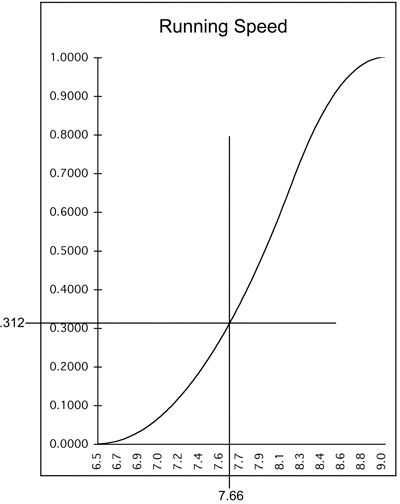
Monte Carlo sampling is an approach that guarantees to respect the shape of the observed pattern over time. A Monte Carlo sampler makes use of past observed data, in the form of a cumulative uncertainty diagram, together with a simple random number generator that picks samples. If you pick enough of them, the bar chart of samples will begin to approximate the pattern of your observed data. The generator is configured to produce random numbers between zero and one. The trick is to use each generated number to pick a value along the vertical of the uncertainty diagram and to draw a horizontal line across. If the first generated number is .312, for example, you draw a horizontal line at .312 on the vertical axis (see the top graph on the next page).
You then draw a vertical line through the point where your horizontal intersects the curve. The value read from the horizontal axis is your first sample point (see the bottom graph on the next page).
The second graph says that for the first sample run, you can expect a speed of 7.66 mph over the course. Now repeat for more random numbers, each one yielding a sample value of speed. If you carry on with this process long enough and make a bar chart of the results, the envelope of the bar chart will begin to approximate the uncertainty diagram you began with (its incremental form).

Simulating the Two-Uncertainty Run
The sampler constructed with this simple rule can now be applied to the running problem. We’ll need two of these samplers, one to give us data points from the speed diagram and the other to give us data points from the distance diagram:

This approach allows us to perform arithmetic on the samples instead of integral calculus on the curves. The first time you invoke this process, it tells you that you ran the course in, for example, 33 minutes. This result is not terribly meaningful—it’s just a calculated time for randomly chosen values from the speed and distance ranges. Using the process over and over, however, will produce a distribution of results that begins to approximate the uncertainty in the expected time of the run.
The diagram shown above is a Monte Carlo simulator for the two-uncertainty problem. It allows you to simulate n instances of the problem and to portray the results in the form of a resultant uncertainty diagram. Here is the result for one hundred instances:

The technique used here is not limited to two uncertainties. It can be used for an entire portfolio of the risks plaguing a software project.
The Software Project Risk Model
RISKOLOGY is a Monte Carlo simulator that we created for the software risk manager. It is a straightforward implementation of Monte Carlo sampling, expressed in spreadsheet logic. We’ve written it in Excel, so you’ll need a legal copy of the program to make use of the tool. RISKOLOGY comes packaged with our own data about some of the risks likely to be facing your project. You can use our data or override with your own.
Download a copy of the RISKOLOGY simulator from our Website:
http://www.systemsguild.com/riskology
Also available there are some templates and instructions for using and customizing the simulator.
A Side-Effect of Using Simulation
Once you’ve simulated sufficient instances of your project, the simulator will provide you with an acceptably smooth output curve. The curve can be made to show the aggregate risks around your project delivery date or around delivered functionality as of a fixed end date. In risk management terms, the result is conveyed as an aggregate risk diagram.
For people who are not in the know about risk management, or for those who have particular difficulty grappling with uncertainty, we suggest that you present it instead as the result of simulation. “We ran this project five hundred times in the simulator,” you might say, “and the result is this”:

“As you can see,” you say, “it shows us delivering before the end of Month 30 only about 15 percent of the time. That doesn’t mean the date is impossible, only that it’s risky. You can count on it with only a 15-percent confidence factor. If you wanted a 75-percent confidence factor, you’d be better off advertising a delivery date in Month 40.”
Alternatives to RISKOLOGY
Our RISKOLOGY simulator is not your only option. There are similar products available for sale. Rather than provide direct pointers here, we will maintain a set at the RISKOLOGY Website (see the URL above). Also described there are at least two meta-risk tools—kits for building your own risk simulators. These products are inexpensive and fairly easily mastered.
Next, as promised, we turn to what we consider the most common, core risks faced by those who run software projects.