
Chapter 2
Introduction to High-Performance Computing
Abstract
This chapter introduces high-performance computing (HPC). High-performance computing is used in every field of science and engineering and cannot be taken for granted. The pioneers of HPC and their contribution are discussed and the world's top five computers are mentioned and discussed in detail. Sparse matrices, libraries necessary to run an HPC environment, such as LAPACK and BLAS, are also discussed in detail.
Keywords
BLAS; Engineering; High-performance computing; LAPACK; Science; Sparse matrix; Top5001. A Short History
“Necessity is the mother of invention” is a famous proverb. Science and technology have led us to a stage in which everything depends on computers. Modern computers are ubiquitous compared with earlier times. Everything is becoming smaller and smarter. Calculations that took half a year to solve now take a month; what took months now takes hours and what took hours now takes minutes. Innovations have also made size increasingly smaller. The big machines of 60–70 years ago, which were called “mainframes,” can be seen on your desktop today. But sky is still the limit, and so after humans created big machines, they created big problems to solve using them. Because every problem has a solution, scientists and engineers have devised ways to run those problems; they have made the machines stronger and smarter and called the machine “supercomputers.” Those giant monsters are state-of-the-art computers that use their magnificent power to solve big “crunchy” problems.
What is a supercomputer? It is a machine that has the highest performance rating at the time of its introduction into the world. But because the world changes dramatically quickly, this means that the supercomputer of today will not be a supercomputer tomorrow. Today, supercomputers are typically a kind of custom design produced by traditional companies such as Cray, IBM, and Hewlett–Packard (HP), which had purchased many of the 1980s companies to gain experience. The first machine generally referred to as a supercomputer was the IBM Naval Ordinance Research Calculator. It was used at Columbia University from 1954 to 1963 to calculate missile trajectories. It predated microprocessors, had a clock speed of 1 μs (1 MHz), and was able to perform about 15,000 operations per second. In the embryological years of supercomputing, the Control Data Corps (CDC's) early machines had very fast scalar processors, some 10 times the speed of the fastest machines offered by other companies at that time. Here, it would be unfair to neglect to mention the name of Seymour Cray (Figure 2.1), who designed the first officially designated supercomputer for control data in the late 1960s. His first design, the CDC 6600, had a pipelined scalar architecture and used the RISC instruction set that his team developed. In that architecture, a single central processing unit (CPU) overlaps fetching, decoding, and executing instructions to process one instruction each clock cycle.

Figure 2.1 Seymour Cray. Courtesy of the history of computing project. http://www.tcop.net.
Cray pushed the number-crunching speed with the CDC 7600 before developing four-processor architecture with the CDC 8600. Multiple processors, however, raised operating system and software issues. When Cray left CDC in 1972 to start his own company, Cray Research, he ignored multiprocessor architecture in favor of vector processing. A vector is a single-column matrix, so a vector processor was able to implement an instruction or a set of instructions that could operate on one-dimensional arrays. Seymour then took over the supercomputer market with his new designs, holding the top spot in supercomputing for 5 years (1985–1990).
Throughout their early history, supercomputers remained the province of large governmental agencies and government-funded institutions. The production runs of supercomputers were small and their export was carefully controlled because they were used in critical nuclear weapons research. When the United States (US) National Science Foundation (NSF) decided to buy Japanese-made NEC supercomputer, it was believed to be a nightmare for US technology greatness. But later on, the world saw something different.
The early and mid-1980s saw machines with a modest number of vector processors working in parallel to become the standard. Typical numbers of processors were in the range of four to sixteen. In the later 1980s and 1990s, massive parallel processing became more popular than vector processors that contained thousands of ordinary CPUs.
Microprocessor speed found on desktops had overtaken the computing power of past supercomputers. Video games use the kind of processing power that had previously been available only in government laboratories. By 1997, ordinary microprocessors were capable of over 450 million theoretical operations per second. Today, parallel designs are based on server-class microprocessors such as the Xeon, AMD Opteron, and Itanium, and coprocessors such as NVIDIA Tesla General Purpose Graphics Processing Unit, AMD GPUs, and IBM Cell. Technologists began building distributed and massively parallel supercomputers and were able to tackle operating system and software problems that had discouraged Seymour Cray from multiprocessing 40 years before. Peripheral speeds had increased so that input/output was no longer a bottleneck. High-speed communications made distributed and parallel designs possible. This suggests that the future of vector technology will not survive. However, NEC produced the Earth Simulator in 2002, which uses 5104 processors and vector technology. According to the top 500 list of supercomputers (http://www.top500.org), the simulator has achieved 35.86 trillion floating point operations per second (teraFLOPs).
Supercomputers are used for highly calculation-intensive tasks such as problems involving quantum physics, climate research, molecular modeling (computing the structures and properties of chemical compounds, biological macromolecules, polymers, and crystals), physical simulations (such as simulating airplanes in wind tunnels, simulating the detonation of nuclear weapons, and research on nuclear fusion).
Supercomputers are also used for weather forecasting, Computational Fluid Dynamics (CFD) (such as modeling air flow around airplanes or automobiles), as discussed in the previous chapter, and simulations of nuclear explosions—applications with vast numbers of variables and equations that have to be solved or integrated numerically through an almost incomprehensible number of steps, or probabilistically by Monte Carlo sampling.
2. High-Performance Computing
High-performance computing (HPC) and supercomputing terms are not different. In fact, people use these terms interchangeably. Although the term “supercomputing” is still used, HPC is used much more frequently in the field of science and engineering. High-performance computing is a technology that focuses on the development of supercomputers (mainly), parallel processing algorithms, and related software such as Message Passing Interface and Linpack. High-performance computing is expensive but if we talk about CFD (which is our main focus), HPC is less costly than usual experimentation done in fluid dynamics. High-performance computing is needed in the areas of:
1. Research and development
2. Parallel programming algorithm development
3. Crunching numerical codes
Why do we need that? The answer to this question is simple. It is because we want to solve big problems. The question arises, “How big?” This really needs some justification, which we will explore. Computational fluid dynamics has been maturing in the past 50 years. Scientists want to solve flow, which requires the equations of fluid dynamics. As mentioned in the chapter on CFD, these equations (Navier–Stokes) are partial differential equations (PDEs), which we have been unable to solve completely until now. For this purpose, we use numerical methods, in which PDEs are broken down into a system of algebraic equations. Partial differential equations through numerical methods need a grid or mesh upon which to run. This is the basic root—the mesh, which solely depends on how powerful the machines are that you would need. If simple laminar flow is to be solved, a simple desktop personal computer (PC) will run the job (with a mesh size in the thousands). If a Reynolds Averaged Navier–Stokes (RANS) equation is needed, I can still use a desktop PC with its multiple cores. However, if we want to run unsteady (a time-dependent simulation), we might need a workstation and large storage. This situation is parallel to the case in which the mesh increases from 1 million cells (1 million is sufficient for RANS most of the time), when two workstations may be required. If more complexity is added like, for large eddy simulation, multiple workstations and a large amount of storage will be required. Thus, where to stop depends on our need and the budget the user would have to play with; between them, we can arrive at a reasonable solution. Computational fluid dynamics needs a lot of effort from both the user's end and the computational part. Scientists and engineers are trying to develop methods that take less effort to solve, are less prone to errors, and are computationally less expensive.
3. Top Five Supercomputers of the World
Top500 is a well-known Web site for the HPC community. It is updated annually in June and November by the National Energy Research and Scientific Computing Center, University of Tennessee in Knoxville, Tennessee, US, and the University of Mannheim in Germany. Top500 contains the list of the top 500 supercomputers. It is not possible to discussing all of them here. Interested readers can visit http://www.top500.org. In this chapter, the top five supercomputers will be discussed.
3.1. Tianhe 2 (Milky Way 2)
Tianhe 2 is the second generation of China's National University of Defense Technology's (NUDT's) first HPC, Tianhe 1 (Tianhe means “Milky Way”). Tianhe 2 became the world's number one system, with a peak performance of 33.86 petaFLOPs/s (PFLOP/s) of LINPACK benchmark [1]; in mid-2013. It has 16,000 compute nodes, each carrying two Intel Ivy Bridge Xeon processor chips and three Xeon Phi coprocessor chips. Thus, the total number of cores is 3,120,000. It is not known which model of the two processors was used: for example, the Intel Ivy Bridge Xeon processor is available with six, eight, or even 10 cores. Each of the 16,000 nodes possesses 88 GB memory and the total memory of the cluster is 1.34 PiB. Figure 2.2 shows the Tianhe 2 supercomputer.
Tianhe beat the Titan (the first-place holder before that), offering double peak performance. According to statistics from Top500, China houses 66 of the top 500 supercomputers, which makes it second compared with the US, which has 252 systems in the Top500 ranking. Without doubt, in the next 5 years most of the supercomputers in the Top500 market list will be owned by China.

3.1.1. Applications
The NUDT declared that Tianhe 2 will be used for simulations, analysis, and government security applications (cybersecurity, for example). After it was placed and assembled at its final location, the system had a theoretical peak performance of 54.9 PFLOP/s. The system draws about 17.6 MW of power for this performance. If the total amount of cooling is considered, this amount of power ends up at 24 MW. The system occupies 720 m2 of space.
3.1.2. Additional Specs
The front-end node is equipped with 4096 Galaxy FT-1500 CPUs developed by NUDT. Each FT-1500 has 16 cores and 1.8 GHz clock frequency. The chip has a performance of 144 gigaFLOPs and runs on 65 W.
The interconnect is called TH Express-2 and was also designed by NUDT; and it has fat tree topology carrying 13 switches each with 576 ports.
The operating system (OS) is Kylin Linux. Because Linux has a GNU license it was modified by NUDT for their requirements. The Kylin OS was developed under the name Qilin, which is a mythical beast in China. This 14-year-old OS was initially developed for the Chinese military and other government organizations, but more recently, a version called NeoKylin that was announced in 2010 was developed. Linux resource management is done with Simple Linux Utility for Resource Management.
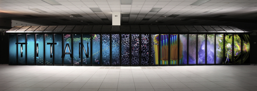
3.2. Titan, Cray XK7
Titan, a Cray XK7 system installed at the Department of Energy's (DOE) Oak Ridge National Laboratory, remains the number two system. It achieved 17.59 PFLOP/s on the Linpack benchmark whereas the theoretical performance was claimed to be 27.1 PFLOP/s. It is one of the most energy-efficient systems on the list, consuming a total of 8.21 MW and delivering 2.143 gigaFLOPs/s per watt (Figure 2.3). On the Green500 list, it ranks third in terms of the energy efficiency rating. It contains more than 18,000 nodes of KX7 with total AMD Opteron 6000 series CPUs with 32 GB of memory and K20X GPU with 6 GB of memory.
XK7 is a state-of-the-art machine that composed of both CPUs and GPUs. Specialized programming scheme required for such a hybrid system will be discussed in Chapter 8. XK7 is the second platform from Cray, Inc to employ a hybrid system. Besides Titan, Cray has also offered the product to the Swiss National Supercomputing Centre, with 272 node machines and Blue.
In the overall architecture of XK7, each blade contains four nodes, each with 1 CPU and 1 GPU per node. The system is scalable to 500 cabinets that can carry 24 blades.
Each CPU contains 16 cores of AMD Opteron 6200 Interlagos series and the GPU model is the Nvidia Tesla K20 Keplar series. Each CPU can be paired with 16 or 32 GB of error-correcting code memory, whereas GPUs can be paired with 5 or 6 GB of memory, depending on the model used. The interconnect is Gemini servicing two nodes with a capacity of 160 GB/s. Power consumption is between 45 and 54 kW for a full cabinet. These cabinets are air- or water-cooled. The OS is SUSE Linux, which can be programmed according to need.
3.3. Sequoia BlueGene/Q
Sequoia, an IBM BlueGene/Q system installed at DOE's Lawrence Livermore National Laboratory (LLNL), is again the number three system. It was first delivered in 2011 and achieved 17.17 PFLOP/s on the Linpack benchmark.
To achieve 17.7 PFLOP/s, Sequoia ran LINPACK for about 23 h with no core failure. However, division leader Kim Cupps, from the owner of the system, LLNL, said that the system is capable of hitting 20 PFLOP/s. In this way, it is more than 80% efficient, which is excellent. She added, “For a machine with 1.6 million cores to run for over 23 h 6 weeks after the last rack arrived on our floor is nothing short of amazing.”
The system consumes 7890 kW of power. Cooling is basically done by running water through tiny copper pipes.
The cluster is extremely efficient for one so large, with 7,890 kW of power, compared with 12,659 kW for the second-best K computer. It is primarily cooled by water running through tiny copper pipes encircling the node cards. Each card holds 32 chips, each of which has 16 cores.
3.3.1. Sequoia's Architecture
The whole system is Linux-based. Computer node Linux runs on 98,000 nodes, whereas Red Hat Enterprise Linux runs on 786 input-output nodes that connect to the file system network.
Use of the Sequoia has been limited since February 2013 because, Kim Cupps said, “To start, the cluster is on a relatively open network, allowing many scientists to use it. But after IBM's debugging process is over around February 2013, the cluster will be moved to a classified network that isn't open to academics or outside organizations. At that point, it will be devoted almost exclusively to simulations aimed at extending the lifespan of nuclear weapons.” She added that “The kind of science we need to do is lifetime extension programs for nuclear weapons, that requires suites of codes running. What we're able to do on this machine is to run large numbers of calculations simultaneously on the machine. You can turn many knobs in a short amount of time.” Figure 2.4 shows the detailed architecture of the Sequoia supercomputer.
Blue Gene/Q uses a PowerPC architecture that includes hardware support for transactional memory, allowing more extensive real-world testing of technology.
In November 2011, in the Top500 list, only three of the top five supercomputers were gaining benefit from GPU. By 2013, more than 60 supercomputers were equipped with GPUs.
Devick Turek, IBM Vice President of High Performance Computing, said that “The use of GPUs in supercomputing tends to be experimental so far; the objective of this is to do real science.”
3.4. K-Computer
Fujitsu's K-Computer, installed at the RIKEN Advanced Institute for Computational Science (AICS) in Kobe, Japan, is the number four system with 10.51 PFLOP/s on the Linpack benchmark. The K-supercomputer has been included in the top of the list in June 2011, Figure 2.5. The K-supercomputer is a Japanese supercomputer. The K-supercomputer has 68,544 CPUs, each with eight cores. This is twice as many as any other supercomputer on the Top500. The letter “K” is short for the Japanese word Kei, which means “Ten Quadrillions.” Thus, the K-Computer is capable of performing 8 quadrillion calculations per second. It contains more than 800 racks. In 2004, the Earth Simulator was the world's fastest computer (with a speed of about 36 teraFLOPs); in June 2011, Japan has held the first position for the first time in world ranking. Something strange thing about the K-Computer was that, like other top supercomputers, it contained neither NVIDIA cores nor the conventional x86 processors from Intel or AMD. It used Fujitsu-designed SPARC processors. The late Hans Warner Meuer (died in 2014) and Ex-Chairman of International Super Computers said, “The SPARC architecture breaks with a couple of trends which we have seen in the last couple of years in HPC and the Top500. It is a traditional architecture in the sense it does not use any accelerators. That's the difference compared to the number two and number four systems, which both use NVIDIA accelerators. The SPARC architecture breaks with a couple of trends which we have seen in the last couple of years in HPC and the Top500.”

Figure 2.4 Sequoia packaging hierarchy. Courtesy of LLNL and Top500.org.
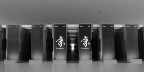
Figure 2.5 K-computer. Courtesy of Top500.org.
These sophisticated Japanese computers are also energy efficient. Although it is surprisingly power hungry and pulls over 9.8 MW of power to make its computations, the system is the second most power-efficient system in the entire Top500 list. In comparison, Rackspace's main UK data center consumes 3.3 MW. Hans Meuer told the audience at a conference, “It's not because of inefficiencies; it's simply driven by its size. It's very large computer.” Based on developments, Meuer added that the ISC expected a system to reach an exaFLOP/s by around 2019. Intel General Manager of Data Centers, Kirk Skaugen said in a conference briefing, “It has impressive efficiency for sure, but it already uses up half the power at around 8 PFLOP/s of what we're going to try and deliver with 1,000 PFLOP/s [in 2018].” [2].
Another interesting feature of the K-Computer is the mesh-tours network to pass information between processes. The topology is designed so that each node is connected to six others, and individual computing jobs can be assigned to a number of interconnected processors. In addition, the Japanese machine uses an HPC six-dimensional mesh-torus network to pass information between processors. The network topology means that every computing node is connected to six others, and individual computing jobs can be assigned to groups of interconnected processors, at which point it will have around 15% more processors.
3.5. Mira, BlueGene/Q system
Mira, a BlueGene/Q system, is the fifth in the world, with 8.59 PFLOP/s on the LINPACK benchmark. The IBM Blue Gene/Q supercomputer, at the Argonne Leadership Computing Facility, is equipped with 786,432 cores and 768 terabytes of memory and has a peak performance of 10 PFLOP/s. Mira's 49,152 compute nodes have a PowerPC A2 1600-MHz processor containing 16 cores, each with four hardware threads, running at 1.6 GHz, and 16 GB of DDR3 memory. A 17th core is available for the communication library. The system nodes are connected in 5D torus topology and the hardware covered area is 1632 ft2.
The system contains a quad Floating Point Unit (FPU) that can be used to execute scalar FPU. The Blue Gene/Q system also features a quad FPU that can be used to execute scalar floating point instructions, four-wide SIMD instructions, or two-wide complex arithmetic SIMD instructions. This quad FPU provides higher single-thread performance for some applications.
The file system is a general parallel file system that has a capacity of 24 PB and 240 GB/second bandwidth. All of these resources are available through high-performance networks including ESnet's recently upgraded 100-GB/s links [3]. The system is shown in Figure 2.6.
The performance of the world's five top supercomputers is listed in Table 2.1.
Since the advent of the IBM roadrunner, which touched the barrier of PFLOP/s in 2008, speed has become a yardstick to measure the performance of the world's supercomputers even until now. The next generation of these supercomputers has to cross the exa-scale line; all of the leading companies, such as HP, Dell, IBM, and Cray, are working hard to achieve massive exa-scale supercomputing.
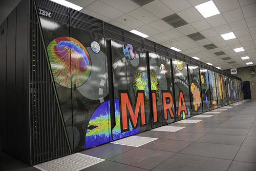
Table 2.1
Peak performance of the top five supercomputers
| Tianhe 2 | Titan, Cray XK 7 | Sequoia | K-Computer | Mira, BlueGene | |
| System family | Tianhe | Cray XK7 | IBM BlueGene/Q | K-Computer | BlueGene |
| Installed at | NUDT | DOE's Oak Ridge National Laboratory | LLNL | AICS | Argonne Leadership Computing Facility |
| Application area | Research | Research | Research | Research | Research |
| Operating system | Linux (Kylin) | Linux | Linux | Linux | Linux |
| Peak performance | 33.86 PFLOP/s | 17.59 PFLOP/s | 17.17 PFLOP/s | 10.51 PFLOP/s | 8.59 PFLOP/s |

4. Some Basic but Important Terminology Used in HPC
When a cluster is ready to run, a few steps are still needed to check its performance before particular applications are started. There are two steps in this regard: the first is the testing phase of the hardware and the second is benchmarking to make sure that the desired test requirements are met. For this purpose, several terms are used in HPC, so the reader must be familiar with them.
4.1. Linpack
Linpack is a code for solving matrices of linear equations and least-square problems. Linpack consists of FORTRAN subroutines and was conventionally used to measure the speed of supercomputers in FLOP/s. The term later overlapped with “linear algebra package” (LAPACK). LAPACK benchmarks are system floating point computing power. The scheme was introduced by Jack Dongarra and was used to solve an N × N system of linear equations of the form Ax = b. The solution was then obtained using the conventional Gaussian elimination method but with partial pivoting. Floating point operations are 2/3N3 + 2N2, the results of which are presented in the form of FLOP/s. There have been some drawbacks to Linpack because it does not push the interconnect between nodes, but focuses on floating point arithmetic units and cache memory. Thom Dunning, Director of the National Center for Supercomputing Applications, said about Linpack: “The Linpack benchmark is one of those interesting phenomena—almost anyone who knows about it will decide its utility. They understand its limitations but it has mindshare because it's the one number we've all bought into over the years” [4].
The Linpack benchmark is a CPU- or compute-bound algorithm. Typical efficiency figures are between 60% and 90%. However, many scientific codes do not feature the dense linear solution kernel, so the performance of this Linpack benchmark does not indicate the performance of a typical code. A linear system solution through iterative methods, for instance, is much less efficient in an FLOP/s sense, because it is dominated by the bandwidth between CPU and memory (a bandwidth-bound algorithm).
4.2. LAPACK
The basic issue in CFD is storage of data. Data are usually in the form of linear equations that are compacted in matrix form. If you are an undergraduate, you have learned that linear equations can easily be written in matrix form and then solved either using iterative or direct methods. In a similar manner, a computer uses these methods to solve matrices.
4.2.1. Matrix Bandwidth and Sparse Matrix
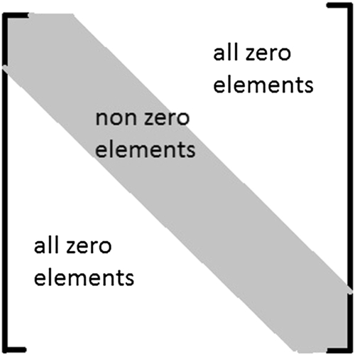
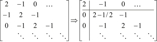
In the case of implicit methods, the values of a variable at all points are computed at a new time step with a single value known at a previous time step. In this way, because there are many unknowns, the number of equations (which is only one), matrix is formed and solved with various procedures. If the approximation (the number of points taken to solve the difference equation) is three points, the matrix would be tri-diagonal. In the case of a five-point approximation, the matrix would be pent-diagonal. This means that the matrix would contain elements necessarily lying along diagonal to as well as one strip above and below it in the case of tri-diagonal, or two in the case of pent-diagonal; the rest of the elements in the matrix are zero. Such a matrix is called a sparse (widely open) matrix. In HPC, we take the advantage of this zero matrix operation.
The matrix form is shown in Figure 2.7. Here, the dominant elements lie in the diagonal stream. In terms of computing, what happens is that the diagonals are stored consecutively in memory. If the matrix is tri-diagonal with a three-point stencil, we can name the diagonal strip just from the first row, first column; then the top strip is a super-strip and the bottom strip is a sub-strip. The most economical storage scheme is 2n – 2 elements consecutively.
The bandwidth of a matrix is defined as b = k1 + k2 + 1, where k1 is the left diagonal(s) below the main diagonal and k2 is the right diagonal(s) above the main diagonal that was mentioned as the sub-strip and super-strip just above. So if k1 = k2 = 0 then the matrix is diagonal only while if k1 = k2 = 1 then matrix is called tri-diagonal. However, if a matrix has dimensions n × n and bandwidth b, then for storage the matrix would be n × b. For example, consider the following matrix:
In the case of diagonal storage, the computer shifts the first row toward the right, making the first element zero; i.e., for the above case, it would be a 6 × 3 matrix
where the first and last elements represent the zero upper right and lower left triangles, respectively. For conversion between array elements A(i,j) and matrix elements Aij, this can be easily done in Fortran. If we allocate the array with dimension
dimension A(n,−1:1)
the main diagonal Aii is stored in A(∗,0). For instance, A(2,0) is similar to a21. The next location in the same row of matrix A would be A(2,1), which is similar to a22. We can write this in a general format as
A(1,j) ∼ ai,i+j
4.2.2. Lower Upper (LU) Factorization
As mentioned earlier, LAPACK is the linear algebra package. The package contains subroutines for solving systems of simultaneous linear equations, least-square solutions of linear systems of equations, eigenvalue, and singular value problems. LAPACK software for linear algebra works on an LU factorization routine that overwrites the input matrix with the factors.
The original goal of LAPACK was for Linpack libraries to run efficiently on shared memory vector and parallel processors. LAPACK routines are written so that, as much as possible, computations are performed by calling up a library called Basic Linear Algebra Sub-programs (BLAS). The BLAS helps LAPACK to achieve high performance with the aid of portable software.
Certain levels of operations are built into these libraries: levels 1, 2, and 3. Level 1 performs vector operations. Level 2 performs matrix–vector operations such as matrix vector product and implicit calculations such as LU decomposition. Level 3 defines matrix–matrix operations, most notably the matrix–matrix product. LAPACK uses the blocked operations of BLAS level 3. This is surely to achieve high performance on cache-based CPUs. However, with modern supercomputers, several projects have come up that extended LAPACK functionality to distributed computing, such as Scalapack and PLapack (Parallel LAPACK) [5].
4.2.3. LU Factorization of Sparse Matrices
Consider a tri-diagonal matrix, as shown below. Applying Gaussian elimination will lead to a second row in which one element is eliminated. One important point is that the zero elements did not become disturbed owing to Gaussian operation. Second, the operation did not affect the tri-diagonality of the matrix. The treatment suggests that L + U factorization takes the same amount of memory as the previous method; however, the case is not limited to tri-diagonal matrices.
4.2.4. Basic Linear Algebra Sub-program Matrix Storage
Following are key factors on the basis of which matrices are stored in BLAS and LAPACK.
4.2.4.1. Array Indexing
In a FORTRAN environment, 1-based indexing is used, whereas C/C++ routines usually use index arrays such pivot points in LU factorization.
4.2.4.2. FORTRAN Column Major Ordering
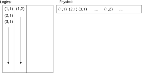
FORTRAN stores the indices in the form of column priority, i.e., elements in a column are stored consecutively. Informally, programmers call thus this trick “the leftmost varies quickest.” See Figure 2.8 for how the elements are stored.
4.2.4.3. Submatrices and Leading Dimension of A Parameter
Using the above storage scheme, it is evident how to store an m×n matrix in mn memory locations. But, there are many cases in which software needs access to a matrix that is a sub-block of another, larger matrix. The sub-block is no longer being shared in memory, as can be seen in Figure 2.9. The way to describe this is to introduce a third parameter in addition to M, N: the leading dimension of A, or the allocated first dimension of the surrounding array, which is illustrated in Figure 2.10.


Now, suppose that you have a matrix A of size 100×100 which is stored in an array 100×100. In this case LDA is the same as m. Now suppose that you want to work only on the submatrix A(91:100, 1:100); in this case the number of rows is 10 but LDA=100. Assuming the fortran column-major ordering (which is the case in LAPACK), the LDA is used to define the distance in memory between elements of two consecutive columns which have the same row index. If you call B = A(91:100, 1:100) then B(1,1) and B(1,2) are 100 memory locations far from each other according to the following formula, B(i,j)=i+(j−1)∗LDA, implies that, B(1,2)=1+(2−1)∗100= 101th location in memory.
4.2.5. Organization of Routines in LAPACK
LAPACK is organized through three levels of routines:
1. Drivers. These are powerful, top-level routines for problems such as solving linear systems or computing a singular value decomposition (SVD). In linear algebra, the SVD is a decomposition of a real or complex matrix. It is mostly used in scientific computing and statistics. Formally, the singular value decomposition of an m × n real or complex matrix M is a factorization of the form M = UΣV∗, where U is an m × m real or complex unitary matrix, meaning that UU∗ = I, Σ is an m × n rectangular diagonal matrix with non-negative real numbers on the diagonal, and V∗ (the conjugate transpose of V, or simply the transpose of V if V is real) is an n × n real or complex unitary matrix. The diagonal entries Σi,i of Σ are known as the singular values of M. The m columns of U are called the left-singular vectors and the n columns of V are called the right-singular vectors of M.
3. Auxiliary routines:
Routines conform to a general naming scheme: XYYZZZ where,
X is the precision: S, D, C, Z stands for single and double, single complex and double complex, respectively.
YY is the storage scheme: general rectangular, triangular, and banded. It indicates the type of matrix (or the most significant matrix). Most of these two-letter codes apply to both real and complex matrices; a few apply specifically to one or the other.
BD: Bi-diagonal.
DI: Diagonal.
GB: General band.
GE: General (i.e., asymmetric or rectangular).
GG: General matrices, generalized problem (i.e., a pair of general matrices).
GT: General tri-diagonal.
HB: (Complex) Hermitian band.
HE: (Complex) Hermitian.
HG: Upper Hessenberg matrix, generalized problem (i.e., a Hessenberg and a triangular matrix).
HP: (Complex) Hermitian, packed storage.
HS: Upper Hessenberg.
OP: (Real) orthogonal, packed storage.
OR: (Real) orthogonal.
PB: Symmetric or Hermitian positive definite band.
PO: Symmetric or Hermitian positive definite.
PP: Symmetric or Hermitian positive definite, packed storage.
PT: Symmetric or Hermitian positive definite tri-diagonal.
SB: (Real) symmetric band.
SP: Symmetric, packed storage.
ST: (Real) symmetric tri-diagonal.
SY: Symmetric.
TB: Triangular band.
TG: Triangular matrices, generalized problem (i.e., a pair of triangular matrices).
TP: Triangular, packed storage.
TR: Triangular (or in some cases quasi-triangular).
TZ: Trapezoidal.
UN: (Complex) unitary.
ZZZ is the matrix operation. They indicate the type of computation performed. For example, SGEBRD is a single precision routine that performs a bi-diagonal reduction BRD of a real general matrix. If it is in qrf form, the factorization is QR factorization, and for lqf it is LQ factorization. Thus, the routine sgeqrf forms the QR factorization of general real matrices in single precision; consequently, the corresponding routine for complex matrices is cgeqrf.
The names of the LAPACK computational and driver routines for the FORTRAN 95 interface in an Intel compiler are the same as FORTRAN 77 names but without the first letter that indicates the data type. For example, the name of the routine that forms the QR factorization of general real matrices in the FORTRAN 95 interface is geqrf. Handling different data types is done by defining a specific internal parameter referring to a module block with named constants for single and double precision.
..................Content has been hidden....................
You can't read the all page of ebook, please click here login for view all page.