
Chapter 6
HPC Benchmarks for CFD
Abstract
This chapter is about the use of high-performance computing in computational flow dynamics, a real devourer of resources. Various types of comparative studies are analyzed in detail and commented on in terms of interconnectivity, storage, and memory requirements. The ANSYS® Fluent®, CFX®, and OpenFOAM benchmarks provide an overview of the nature of problems run on the various types of hardware.
Keywords
ANSYS CFX; ANSYS FLUENT; Benchmarks; CFD; HPC; OpenFOAM1. How Big Should the Problem Be?
Computational Fluid Dynamics (CFD) problems are resource-hungry applications. They require a large amount of computer power to be solved. Let us start with the smallest problem. Consider a one-dimensional (1D) partial differential equation. To solve it, you would need at least three points. For its first-order accurate solution, these three points in space and a certain number of points (for example, 300) for time steps are needed. A single core processor such as Pentium IV with 512 MB RAM will easily solve it in a few minutes. Now, add some complexity: make it 2D and go for more grid points. This would need more computational power, such as 1 GB memory. Now, make it 3D and solve the Navier–Stokes equation with 0.5 million grid points. This would add more complexity and you would need at least a dual-core processor and 2 GB RAM. For Reynolds-averaged Navier–Stokes (RANS) simulations this is a reasonably good machine. This may not be of paramount importance because for real physics one may need to capture turbulence. For this, it will become mandatory to add turbulence model to the simulation.
For wall-bounded flows, whether internal or external, the mesh is kept fine near the wall to capture near-wall viscous effects, whether turbulent or laminar. From the viewpoint of computational expense, the mesh is usually stretched in terms of geometric progression near the wall, which can make cell size very large at the far field boundaries. Ideally, one should keep all the points equally spaced, but this can make mesh size very fine. Even in the case of mesh stretching when the mesh size has been increased, a dual-core PC would also be useless. The user may require a quad core with 64-bit architecture support so that he or she can use the whole 4 GB of RAM, at least if the operating system is 32-bit. To get maximum power out of your computer, all four cores can be used. In summary, it can be said that high power is required when:
1. There is a 3D problem to solve
2. There is a need to solve turbulence
Table 6.1
Number of cores suitable for a particular mesh size for Fluent simulation
| Cluster size (no. of cores) | Fluent case size (no. of cells/mesh size) | No. of simultaneous Fluent simulations |
| 8 | Up to 2–3 million | 1 |
| 16 | Up to 2–3 million | 2 |
| 16 | Up to 4–5 million | 1 |
| 32 | Up to 8–10 million | 1 |
| 32 | Up to 4–5 million | 2 |
| 64 | Up to 16–20 million | 1 |
| 64 | Up to 8–10 million | 2 |
| 64 | Up to 4–5 million | 4 |
| 128 | Up to 30–40 million | 1 |
| 256 | Up to 70–100 million | 1 |
| 256 | Up to 30–40 million | 2 |
| 256 | Up to 8–10 million | 4 |
| 256 | Up to 4–5 million | 16 |
4. There is unsteady flow
5. There is a need for direct numerical simulation, large eddy simulations (LES), or detached eddy simulations (DES).
Thus, an obvious question is how big the problem must be to run on a cluster for HPC. Performance benchmarks are done for this purpose. Guidelines based on the number of cores to be used with respect to the problem size are given in Table 6.1. The benchmark was performed on Sun machines [1]. It is common to see performance benchmarks for CFD with mesh size limits crossing 100 million grid points.
2. Maximum capacity of the critical components of a cluster
2.1. Interconnect
Interconnect sometimes becomes a bottleneck in the performance of a cluster. This becomes tiring especially when one does not understand where the problem is because everything looks fine in terms of functionality. A fast interconnect usually solves the problem. The term “low latency high bandwidth” is used in the networking field; it means that the time for communication between nodes must be as low as possible and the data transfer rate must be high, i.e., large data packets can be transferred in no time. Currently, the largest vendor of Infiniband in the world is the Mellanox.
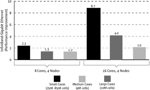
Figure 6.1 shows a performance histogram for the ratio of Infiniband to gigabit Ethernet. Again, the reference benchmark has been used with respect to the Sun machine [1] with ANSYS® Fluent, v. 12 (thanks to Sun, Inc.). The curve has two parts: one is for four nodes each of eight core processors and the other is for four nodes with 16 cores each. The curve is self-explanatory. For a smaller number of cores, a low-size mesh gives subsequent performance but the performance decays and the ratio is increased with the problem size. The ratio of Infiniband to gigabit does not show high values, which indicates that for a low to medium-size mesh (4–10 million), if there is a smaller number of cores, using gigabit Ethernet is sufficient. If the number of cores is increased, Infiniband will have an impact. The first bar has a peak at 8.7, which means that it has an advantage when the number of cores is larger. Consequently, the bars shorten with an increase in problem size because of the large amount of data transfer between nodes. Obviously, the calculations increase as the mesh size increases.
2.2. Memory
Memory requirements for the test cases span from a few hundred megabytes to about 25 GB. As the job is distributed over multiple nodes, the memory requirements per node are reduced correspondingly. As a starting point, 2 GB per core (e.g., 8 GB per dual-processor, dual-core node) is recommended. The total memory requirement for one Fluent 12 simulation on the cluster (distributed across multiple nodes) can scale linearly with the Fluent model size (measured in number of cells) and can be on the order of the estimates listed in Table 6.2. The author has personally noticed that for steady simulations in almost all versions from 6 to 14, Fluent consumes memory only while reading the case and data files and when it is distributing the mesh over the compute nodes. Figure 6.2 shows the performance of DDR with respect to the software-defined ratio for different meshes on Sun clusters on Fluent 12. The best performance can be obtained with a larger number of cores for a heavy mesh or with an intermediate number of cores on a medium mesh.
2.3. Storage
Adequate storage capacity is also required to run ANSYS Fluent. Data file sizes created by ANSYS Fluent differ with the CFD simulation model size, which is usually measured by the number of cells. With unsteady simulations, the typical data file size increases because of the increasing amount of data to store at each time step. Typical file sizes for a steady case are shown in Table 6.3.
3. Commercial Software Benchmarks
3.1. ANSYS Fluent Benchmarks
ANSYS Fluent has several benchmarks available [2]. These benchmarks are versatile in that they contain problems of different scales and have been tested on a number of different platforms. These have been included here so that the reader can have an idea about how the problem depends on the type of hardware used. ANSYS defines benchmarks in terms of the performance rating, speedup, and efficiency. The definition of each term is given below:
1. Performance Rating: The performance rating is the basic measure used to report performance results of ANSYS Fluent benchmarks. It is defined as the number of benchmarks that can be run on a given machine (in sequence) in a 24 h period. It is computed by dividing the number of seconds required to run the benchmark by the number of seconds in a day (86,400 s). A higher rating means faster performance.
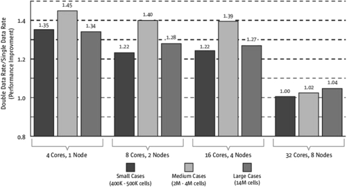
Table 6.3
Storage needs for a particular problem setup in ANSYS Fluent
| Fluent case size (no. of cells/mesh size) | Space requirements |
| 2 Million | 200 MB |
| 5 Million | 1 GB |
| 50 Million | 5 GB |
2. Speedup: Speedup is the ratio of wall-clock time required to complete a give calculation using a single processor compared with that of the equivalent calculation performed on a concurrent machine. Its value ranges from 0 to the number of processors used for the parallel run. When speedup is equal to the number of processors used, it is called perfect or linear. Sometimes speedup exceeds the number of processors. This is referred to as super-linear speedup and is often caused by the availability and use of larger amounts of fast memory (e.g., cache or local memory) compared with a single processor run.
3. Efficiency: Efficiency is speedup normalized by the number of processors used, presented as a percentage. It indicates the overall use of the central processing units (CPUs) during a parallel calculation. An efficiency of 100% indicates that each CPU is completely occupied by computation during the run period and corresponds to linear speedup. An efficiency of 60% indicates that each CPU is performing useful computation only 60% of the time. The remaining time is spent waiting for other functions, such as parallel communication or work on other processors, to complete. The curves will be shown for the benchmarks with respect to the performance rating and not the standard speedup. The reason is that for speedup performance is measured on the basis of a serial process that is not possible until the benchmark is performed on a single core. Because the technology has made a core to act as a single CPU and in most machines each processor chip contains a minimum of four cores, sometimes it is not possible to measure performance on the basis of a single core, as in most IDM machines. The performance rating thus gives an equivalent measure of speedup with almost the same trend as that depicted in the usual speedup curves.
3.1.1. Flow of Eddy Dissipation
The eddy case consists of the flow modeling of reacting flow with an eddy-dissipation model such as k-ε. Here, ANSYS Fluent has used the k-ε model along with an implicit solver. It has been reported in [2] that this simulation was attempted with 417,000 cells and all-structured mesh. The benchmark results are shown in Figure 6.3. Three machines and their different configurations were used, including the famous hardware of Bull, Fujitsu, and IBM. For the Bull machine, the model was B710 with an Intel E5-2680 processor with a speed of 2.8 GHz with turbo-boost on, and the operating system was Redhat 6 with connectivity of FDR Infiniband by Mellanox. Two models of Fujitsu were tested, each with a difference in CPU speed of 2.7 and 3 GHz, respectively. IBM machines also differ in CPU rating; one is IBM DX 360 M3 with a 2.6 GHz processor and the other is IBM DX360 M4 with a 2.7 GHz processor. All used the same operating system, Redhat Linux 6, and FDR Infiniband of Mellanox for connectivity.
If you look carefully at Figure 6.3, you will see that IBM machine with a 2.6 GHz processor is taking the lead. However, that this machine started at 16 cores at a minimum, which means that the problem is not large enough to require a high number of cores. This is indicated by 256 cores, showing that all of the curves are fading; this is not true with the IBM with a 2.6 GHz processor, which is still a bit straight on 1024 cores compared with others. Table 6.4 mentions other parameters that were described previously. The core solver speedup and core solver efficiency are also listed. ANSYS Fluent described solver efficiency on one core as 100% because there are no communication bottlenecks and no shared memory headache. Because the solver speedup and efficiency are tabulated with respect to a single core, the columns are shown as not applicable (N/A) for IBM machines, because the minimum number of cores is 16.

Table 6.4
Core solver rating, core solver speedup, and efficiency details for the problem of eddy dissipation
| Processes | Machines | Core solver rating | Core solver speedup | Core solver efficiency |
| Bull with 2.8 GHz turbo | ||||
| 1 | 1 | 243.9 | 1 | 100% |
| 20 | 1 | 2773.7 | 11.4 | 57% |
| 40 | 2 | 4753.8 | 19.5 | 49% |
| 80 | 4 | 7125.8 | 29.2 | 37% |
| 160 | 8 | 9846.2 | 40.4 | 25% |
| 320 | 16 | 11,443.7 | 46.9 | 15% |
| Fujitsu with 2.7 GHz processor | ||||
| 1 | 1 | 185.4 | 1 | 100% |
| 2 | 1 | 361.1 | 1.9 | 97% |
| 4 | 1 | 661.3 | 3.6 | 89% |
| 8 | 1 | 1185.6 | 6.4 | 80% |
| 10 | 1 | 1470.6 | 7.9 | 79% |
| 12 | 1 | 1489.7 | 8 | 67% |
| 24 | 1 | 2421.9 | 13.1 | 54% |
| 48 | 2 | 4670.3 | 25.2 | 52% |
| 96 | 4 | 7697.1 | 41.5 | 43% |
| 192 | 8 | 9573.4 | 51.6 | 27% |
| Fujitsu with 3 GHz processor | ||||
| 1 | 1 | 206.4 | 1 | 100% |
| 2 | 1 | 402 | 1.9 | 97% |
| 4 | 1 | 756.7 | 3.7 | 92% |
| 8 | 1 | 1318.1 | 6.4 | 80% |
| 10 | 1 | 1644.1 | 8 | 80% |
| 20 | 1 | 2769.2 | 13.4 | 67% |
| 40 | 2 | 5112.4 | 24.8 | 62% |
| 80 | 4 | 8093.7 | 39.2 | 49% |
| 160 | 8 | 7819 | 37.9 | 24% |
| 320 | 16 | 8037.2 | 38.9 | 12% |
| IBM with 2.6 GHz processor | ||||
| 16 | 1 | 2168.1 | N/A | N/A |
| 24 | 2 | 3083 | N/A | N/A |
| 32 | 2 | 3945.2 | N/A | N/A |
| 48 | 3 | 5228.4 | N/A | N/A |
| 64 | 4 | 6376.4 | N/A | N/A |
| 96 | 6 | 7783.8 | N/A | N/A |
| 128 | 8 | 9118.7 | N/A | N/A |
| 384 | 24 | 9959.7 | N/A | N/A |
| 1024 | 64 | 11,220.8 | N/A | N/A |
| Table Continued | ||||

| Processes | Machines | Core solver rating | Core solver speedup | Core solver efficiency |
| IBM with 2.7 GHz processor | ||||
| 16 | 1 | 2341.5 | N/A | N/A |
| 32 | 2 | 4148.9 | N/A | N/A |
| 48 | 2 | 5693.6 | N/A | N/A |
| 64 | 3 | 6996 | N/A | N/A |
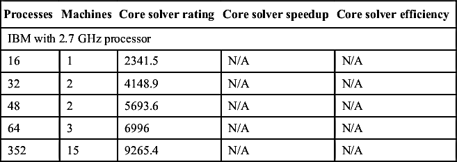
| 352 | 15 | 9265.4 | N/A | N/A |
3.1.2. Flow Over Airfoil
Figure 6.4 shows benchmarking for the case of flow over an airfoil with about 2 million cells. All of the cells used in the simulation were hexahedral. The turbulence model used was realizable k-ε with a density-based implicit solver. Based on the solver rating, Fluent scales up very well for a higher number of cores. The problem of 2 million, however, dictates that almost all of the curves start to decelerate after 256 cores. This means that for this problem on all of the machines tested, 256 cores are enough. No significant increase in performance is expected if the cores are extended beyond this number. In comparison, IBM has slightly better performance than Fujitsu and Bull. Table 6.5 shows the results of core solver rating, speedup, and efficiency.

Table 6.5
Core solver rating, core solver speedup, and efficiency details for the problem of flow over aircraft
| Processes | Machines | Core solver rating | Core solver speedup | Core solver efficiency |
| Bull with 2.8 GHz turbo | ||||
| 1 | 1 | 210.3 | 1 | 100% |
| 20 | 1 | 2583 | 12.3 | 61% |
| 40 | 2 | 4958.4 | 23.6 | 59% |
| 80 | 4 | 9340.5 | 44.4 | 56% |
| 160 | 8 | 15,853.2 | 75.4 | 47% |
| 320 | 16 | 22,012.7 | 104.7 | 33% |
| Fujitsu with 2.7 GHz processor | ||||
| 1 | 1 | 164.9 | 1 | 100% |
| 2 | 1 | 329.9 | 2 | 100% |
| 4 | 1 | 640.4 | 3.9 | 97% |
| 8 | 1 | 1092.3 | 6.6 | 83% |
| 10 | 1 | 1442.4 | 8.7 | 87% |
| 12 | 1 | 1757 | 10.7 | 89% |
| 24 | 1 | 2921.4 | 17.7 | 74% |
| 48 | 2 | 5374.8 | 32.6 | 68% |
| 96 | 4 | 9735.2 | 59 | 61% |
| 192 | 8 | 14,521 | 88.1 | 46% |
| 384 | 16 | 25,985 | 157.6 | 41% |
| Fujitsu with 3 GHz processor | ||||
| 1 | 1 | 184.2 | 1 | 100% |
| 2 | 1 | 368.5 | 2 | 100% |
| 4 | 1 | 719.1 | 3.9 | 98% |
| 8 | 1 | 1327.2 | 7.2 | 90% |
| 10 | 1 | 1575.2 | 8.6 | 86% |
| 20 | 1 | 2721.3 | 14.8 | 74% |
| Table Continued | ||||

| Processes | Machines | Core solver rating | Core solver speedup | Core solver efficiency |
| 40 | 2 | 4979.8 | 27 | 68% |
| 80 | 4 | 7500.3 | 43 | 50% |
| 160 | 8 | 16,225.4 | 88.1 | 55% |
| 320 | 16 | 25,600 | 139 | 43% |
| IBM with 2.6 GHz processor | ||||
| 16 | 1 | 2076.9 | N/A | N/A |
| 24 | 2 | 3110.7 | N/A | N/A |
| 32 | 2 | 3958.8 | N/A | N/A |
| 48 | 3 | 5877.6 | N/A | N/A |
| 64 | 4 | 7697.1 | N/A | N/A |
| 96 | 6 | 11,041.5 | N/A | N/A |
| 128 | 8 | 14,163.9 | N/A | N/A |
| 256 | 16 | 22,887.4 | N/A | N/A |
| 384 | 24 | 27,212.6 | N/A | N/A |
| 512 | 32 | 30,315.8 | N/A | N/A |
| IBM with 2.7 GHz processor | ||||
| 16 | 1 | 2192.9 | N/A | N/A |
| 24 | 1 | 3005.2 | N/A | N/A |
| 48 | 2 | 5798.7 | N/A | N/A |
| 64 | 3 | 7731.5 | N/A | N/A |
| 96 | 4 | 11,006.4 | N/A | N/A |
| 128 | 6 | 13,991.9 | N/A | N/A |
| 192 | 8 | 18,782.6 | N/A | N/A |
| 256 | 11 | 22,736.8 | N/A | N/A |
| 360 | 15 | 26,584.6 | N/A | N/A |

3.1.3. Flow Over Sedan Car
The problem of a Sedan car was simulated with about 4 million cells. The actual number of cells was 3.6 million. It was a hybrid grid, obviously, owing to the complexity of the geometry especially in the regions where the car wheel is present. k-ε was used as a turbulence model with a pressure-based implicit solver. Figure 6.5 compares benchmarking for this problem; almost all of the machines behave similarly, but the Bull machine is linear until the end and we can expect performance to continue (if not perfectly) if the cores are extended. The behavior is not drifting away from a linear trend, aside from IBM, which shows the curves for the two machines starting to come down at 1024. However, it is expected that after about one x-axis unit all of the curves will start to come down because the problem size is not extravagant. In this problem case, we can say that Bull performed the best. Table 6.6 tabulates Figure 6.5.

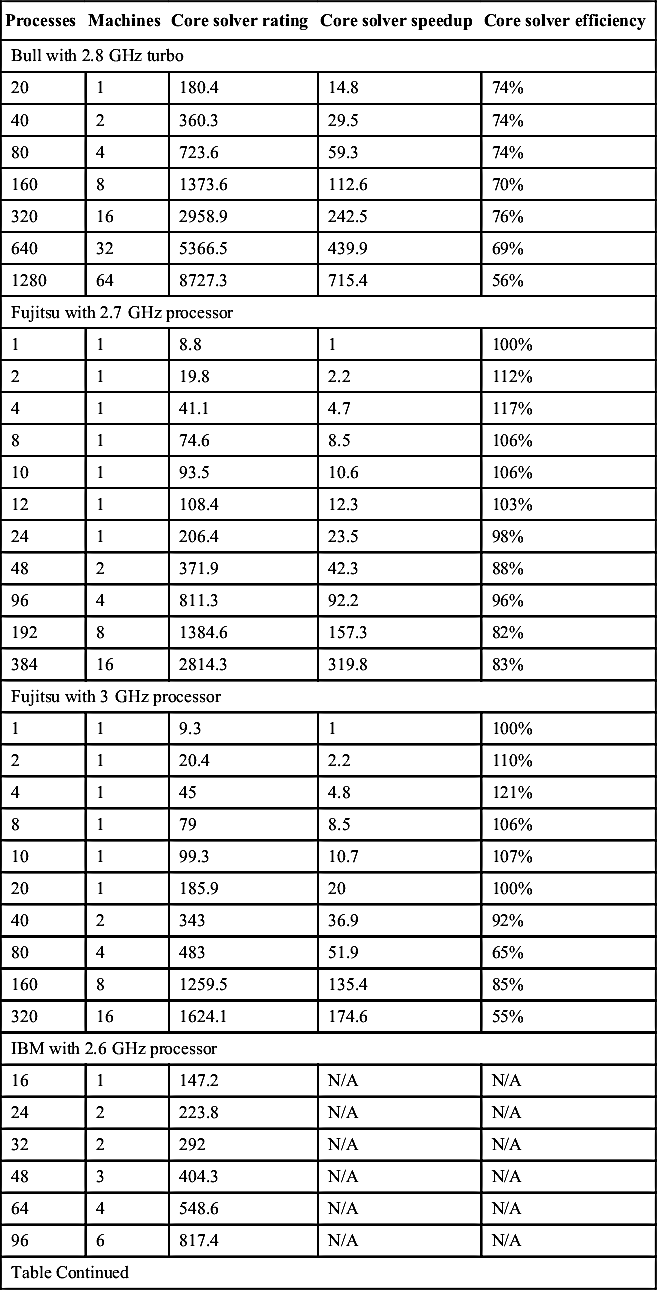
3.1.4. Flow Over Truck Body with 14 Million Cells
A truck is an interesting problem from an aerodynamics point of view. Usually, because of their bulky mass, trucks do not attain high velocity on highways. Hence, their drag is reduced by certain geometrical modifications. For example, a fairing is mounted on the roof to reduce drag and thereby increase speed. Also the base drag decreases the speed many fold. Thus, it is the testing through CFD that tells us the contribution of drag on its performance and true simulation can be performed only using techniques like DES. Therefore, HPC is the best possible solution to run these kind of simulations. The benchmark was performed by ANSYS Fluent on a truck body with about a 14-million hybrid type of grid (Figure 6.6). A pressure-based implicit solver was used for simulations. Details regarding the machines used and the efficiency are shown in Table 6.7. Figure 6.6 also shows that the Bull machine performed better than the others. The curve was almost linear until the end.

Table 6.6
Core solver rating, core solver speedup, and efficiency details for the problem of flow over a sedan car
| Processes | Machines | Core solver rating | Core solver speedup | Core solver efficiency |
| Bull with 2.8 GHz turbo | ||||
| 1 | 1 | 157.4 | 1 | 100% |
| 20 | 1 | 1882.4 | 12 | 60% |
| 40 | 2 | 3818.8 | 24.3 | 61% |
| 80 | 4 | 7663 | 48.7 | 61% |
| 160 | 8 | 15,926.3 | 101.2 | 63% |
| 320 | 16 | 30,315.8 | 192.6 | 60% |
| 640 | 32 | 55,741.9 | 354.1 | 55% |
| Fujitsu with 2.7 GHz processor | ||||
| 1 | 1 | 125.9 | 1 | 100% |
| 2 | 1 | 222 | 1.8 | 88% |
| 4 | 1 | 502.8 | 4 | 100% |
| 8 | 1 | 882.3 | 7 | 88% |
| 10 | 1 | 1175.9 | 9.3 | 93% |
| 12 | 1 | 1125.4 | 8.9 | 74% |
| 24 | 1 | 2053.5 | 16.3 | 68% |
| 48 | 2 | 4085.1 | 32.4 | 68% |
| 96 | 4 | 7944.8 | 63.1 | 66% |
| 192 | 8 | 16,149.5 | 128.3 | 67% |
| 384 | 16 | 29,793.1 | 236.6 | 62% |
| Fujitsu with 3 GHz processor | ||||
| 1 | 1 | 141.2 | 1 | 100% |
| 2 | 1 | 284 | 2 | 101% |
| 4 | 1 | 562.1 | 4 | 100% |
| 8 | 1 | 1066.7 | 7.6 | 94% |
| 10 | 1 | 1269.2 | 9 | 90% |
| 20 | 1 | 1916.8 | 13.6 | 68% |
| 40 | 2 | 3831.5 | 27.1 | 68% |
| 80 | 4 | 7464.4 | 52.9 | 66% |
| 160 | 8 | 14,961 | 106 | 66% |
| 320 | 16 | 27,648 | 195.8 | 61% |
| IBM with 2.6 GHz processor | ||||
| 16 | 1 | 1508.5 | N/A | N/A |
| 24 | 2 | 2285.7 | N/A | N/A |
| 32 | 2 | 3091.2 | N/A | N/A |
| 48 | 3 | 4632.7 | N/A | N/A |
| Table Continued | ||||

| Processes | Machines | Core solver rating | Core solver speedup | Core solver efficiency |
| 64 | 4 | 6149.5 | N/A | N/A |
| 96 | 6 | 9118.7 | N/A | N/A |
| 256 | 16 | 23,351.4 | N/A | N/A |
| 384 | 24 | 32,000 | N/A | N/A |
| 512 | 32 | 38,831.5 | N/A | N/A |
| 1024 | 64 | 54,857.1 | N/A | N/A |
| IBM with 2.7 GHz processor | ||||
| 16 | 1 | 1519.8 | N/A | N/A |
| 24 | 1 | 2068.2 | N/A | N/A |
| 48 | 2 | 4199.3 | N/A | N/A |
| 64 | 3 | 5610.4 | N/A | N/A |
| 96 | 4 | 8307.7 | N/A | N/A |
| 128 | 6 | 11,184.5 | N/A | N/A |
| 192 | 8 | 16,776.7 | N/A | N/A |
| 256 | 11 | 21,735.8 | N/A | N/A |
| 360 | 15 | 29,042 | N/A | N/A |
| 16 | 1 | 1519.8 | N/A | N/A |
| 24 | 1 | 2068.2 | N/A | N/A |

Table 6.7
Core solver rating, core solver speedup, and efficiency details for the problem of flow over a truck body with 14 million cells
| Processes | Machines | Core solver rating | Core solver speedup | Core solver efficiency |
| Bull with 2.8 GHz turbo | ||||
| 20 | 1 | 180.4 | 14.8 | 74% |
| 40 | 2 | 360.3 | 29.5 | 74% |
| 80 | 4 | 723.6 | 59.3 | 74% |
| 160 | 8 | 1373.6 | 112.6 | 70% |
| 320 | 16 | 2958.9 | 242.5 | 76% |
| 640 | 32 | 5366.5 | 439.9 | 69% |
| 1280 | 64 | 8727.3 | 715.4 | 56% |
| Fujitsu with 2.7 GHz processor | ||||
| 1 | 1 | 8.8 | 1 | 100% |
| 2 | 1 | 19.8 | 2.2 | 112% |
| 4 | 1 | 41.1 | 4.7 | 117% |
| 8 | 1 | 74.6 | 8.5 | 106% |
| 10 | 1 | 93.5 | 10.6 | 106% |
| 12 | 1 | 108.4 | 12.3 | 103% |
| 24 | 1 | 206.4 | 23.5 | 98% |
| 48 | 2 | 371.9 | 42.3 | 88% |
| 96 | 4 | 811.3 | 92.2 | 96% |
| 192 | 8 | 1384.6 | 157.3 | 82% |
| 384 | 16 | 2814.3 | 319.8 | 83% |
| Fujitsu with 3 GHz processor | ||||
| 1 | 1 | 9.3 | 1 | 100% |
| 2 | 1 | 20.4 | 2.2 | 110% |
| 4 | 1 | 45 | 4.8 | 121% |
| 8 | 1 | 79 | 8.5 | 106% |
| 10 | 1 | 99.3 | 10.7 | 107% |
| 20 | 1 | 185.9 | 20 | 100% |
| 40 | 2 | 343 | 36.9 | 92% |
| 80 | 4 | 483 | 51.9 | 65% |
| 160 | 8 | 1259.5 | 135.4 | 85% |
| 320 | 16 | 1624.1 | 174.6 | 55% |
| IBM with 2.6 GHz processor | ||||
| 16 | 1 | 147.2 | N/A | N/A |
| 24 | 2 | 223.8 | N/A | N/A |
| 32 | 2 | 292 | N/A | N/A |
| 48 | 3 | 404.3 | N/A | N/A |
| 64 | 4 | 548.6 | N/A | N/A |
| 96 | 6 | 817.4 | N/A | N/A |
| Table Continued | ||||
| Processes | Machines | Core solver rating | Core solver speedup | Core solver efficiency |
| 128 | 8 | 1082.7 | N/A | N/A |
| 256 | 16 | 2112.5 | N/A | N/A |
| 384 | 24 | 3130.4 | N/A | N/A |
| 512 | 32 | 4056.3 | N/A | N/A |
| 1024 | 64 | 6912 | N/A | N/A |
| IBM with 2.7 GHz processor | ||||
| 16 | 1 | 157 | N/A | N/A |
| 24 | 1 | 203.4 | N/A | N/A |
| 48 | 2 | 400 | N/A | N/A |
| 64 | 3 | 539.3 | N/A | N/A |
| 96 | 4 | 799.3 | N/A | N/A |
| 128 | 6 | 1057.5 | N/A | N/A |
| 192 | 8 | 1627.1 | N/A | N/A |
| 256 | 11 | 2138.6 | N/A | N/A |
| 360 | 15 | 2851.5 | N/A | N/A |

3.1.5. Truck with 111 Million Cells
This was the largest benchmark performed by ANSYS Fluent. It consisted of the same problem as discussed before but with 111 million cells. Obviously, with such a huge grid it is difficult to manage the whole grid structure; therefore, mixed-type cells were built. The model was DES turbulence and a pressure base solver was used to solve the governing equations. A perfect linear curve was obtained for Bull machine whereas the worst performance was shown by Fujitsu with a 2.7 GHz processor (see Figure 6.7). Table 6.8 shows the core solver efficiency and speedup.
3.1.6. Performance of Different Problem Sizes with a Single Machine
We have seen that the best machine so far is Bull. We now compare the performance of each problem tested on the Bull machine, shown in Figure 6.8.
Figure 6.8 shows that scalability is good for larger mesh sizes. The smallest mesh of the eddy-dissipation problem, 4000 cells, moves downward after 64 cores. Truck 111 million is still scalable because of the larger mesh size. We can conclude that if one wants to put up a cluster in a laboratory, the first thing is to know the size of the problem size and how large it may be in future. Will you run larger meshes in the future, or unsteady simulations? Then, you need to know, if your possible mesh size may be millions of cells, how many cores would be sufficient. Keeping in mind the components of Infiniband, the operating system, and the MPI software constant, these benchmark curves will guide you as to how many cores will be sufficient for your case. The last step is to select the machine. Keeping the budget in mind, you will select a vendor and then compare prices in the market. If a vendor is the best for your problem but is expensive, go to the next best one, and so on. A flowchart will help you select an appropriate machine, as shown in Figure 6.9.

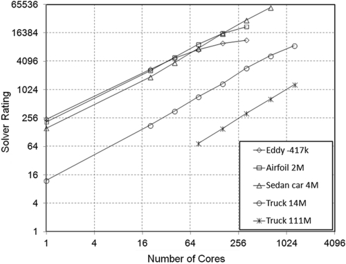
Figure 6.8 Benchmarking for a number of problems on the bull machine with a 2.8 GHz turbo processor.
Table 6.8
Core solver rating, core solver speedup, and efficiency details for the problem of flow over a truck body with 111 million cells
| Processes | Machines | Core solver rating | Core solver speedup | Core solver efficiency |
| Bull with 2.8 GHz turbo | ||||
| 80 | 4 | 74 | N/A | N/A |
| 160 | 8 | 154.2 | N/A | N/A |
| 320 | 16 | 322.7 | N/A | N/A |
| 640 | 32 | 654 | N/A | N/A |
| 1280 | 64 | 1303.2 | N/A | N/A |
| Fujitsu with 2.7 GHz processor | ||||
| 96 | 4 | 56.3 | N/A | N/A |
| 192 | 8 | 110 | N/A | N/A |
| 384 | 16 | 318.5 | N/A | N/A |
| Fujitsu with 3 GHz processor | ||||
| 80 | 4 | 56.3 | N/A | N/A |
| 160 | 8 | 128 | N/A | N/A |
| 320 | 16 | 208.2 | N/A | N/A |
| Table Continued | ||||

| Processes | Machines | Core solver rating | Core solver speedup | Core solver efficiency |
| IBM with 2.6 GHz processor | ||||
| 64 | 4 | 56.7 | N/A | N/A |
| 96 | 6 | 79.6 | N/A | N/A |
| 128 | 8 | 107 | N/A | N/A |
| 256 | 16 | 249.9 | N/A | N/A |
| 384 | 24 | 378.9 | N/A | N/A |
| 512 | 32 | 501.7 | N/A | N/A |
| 1024 | 64 | 998.8 | N/A | N/A |
| IBM with 2.7 GHz processor | ||||
| 64 | 3 | 61.4 | N/A | N/A |
| 96 | 4 | 93 | N/A | N/A |
| 128 | 6 | 121.6 | N/A | N/A |
| 192 | 8 | 185.3 | N/A | N/A |
| 256 | 11 | 246.7 | N/A | N/A |
| 360 | 15 | 348.8 | N/A | N/A |


Alternately, you may obtain quotations from all of the vendors and then compare them and select the best one. You may need to compromise between performance and your budget. Vendors sell their machines mostly on the basis of teraflops per second. This is based on the LINPACK benchmark, but for software such as ANSYS Fluent and CFX or OpenFOAM, you need to look at the number of cores for your problem and choose a machine on this basis. Second, Infiniband is offered by Mellanox, which is the sole vendor in the HPC market, like NVIDIA in GPU technology. Infiniband is expensive equipment, but whatever machine you are going to buy, its price is fixed, so determine whether the vendor is offering it as a package. Otherwise, you will have to make room in the budget for it, as well.
3.2. Benchmarks for CFX
3.2.1. Automotive Pump Simulation
This CFX benchmark was used for an automotive pump problem consisting of 596,252 cells. There were mixed types of elements, including tetrahedrons and prisms. The models used were k-ε and a moving reference frame to inculcate the motion of the rotor and make the stator stationary. A density-based solver was employed in the simulations.
CFX benchmarks differ from ANSYS Fluent benchmarks, in that ANSYS mentions different processor architectures on which the benchmarks are run rather than specifying different vendors. The pump problem was also run with different types of processors, Infiniband architecture, operating systems, etc. The pump problem was mainly run with various Intel processors. The first was with an Intel E5-2670 processor with a 2.6 GHz processor, which had the best performance overall. It had 64 GB RAM per machine and the operating system was Redhat Linux. Next was Intel E5-2680 with a 2.7 GHz processor. This processor was Intel Sandy Bridge, a dual-CPU, 16-core processor with 28 GB RAM and CentOS as the operating system. The last (but not least) was Intel x5650, with a 2.67 GHz processor with 39 GB RAM and SLES as the operating system, as shown in Figure 6.10. The SLES operating system is from SUSE Linux Enterprise Service. This is a much more stable, secure, and user-friendly version of Linux. Figure 6.10 shows the values only for the solver rating; core solver speed and efficiency are listed in Table 6.9.
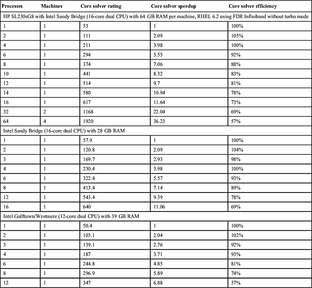
3.2.2. Le Mans Car Simulation
Millions of dollars are spent improving the design of sports cars. Le Mans is an example. The CFX team performed an analysis fn this car using a mesh size of 1,864,025 cells. All of the elements were tetrahedral. The turbulence model was k-ε with a density-based implicit solver. Figure 6.11 shows the benchmark curve and Table 6.10 lists the detailed parameters. Figure 6.11 also shows that Intel E5 2670 depicted a linear trend for even 64 cores, and that this was the best among the three processors tested.
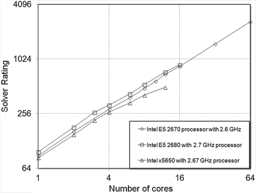
Table 6.9
Benchmarks performed with CFX software for the pump simulation problem
| Processes | Machines | Core solver rating | Core solver speedup | Core solver efficiency |
| HP SL230sG8 with Intel Sandy Bridge (16-core dual CPU) with 64 GB RAM per machine, RHEL 6.2 using FDR Infiniband without turbo mode | ||||
| 1 | 1 | 88 | 1 | 100% |
| 2 | 1 | 162 | 1.84 | 92% |
| 4 | 1 | 285 | 3.24 | 81% |
| 6 | 1 | 381 | 4.33 | 72% |
| 8 | 1 | 483 | 5.49 | 69% |
| 10 | 1 | 580 | 6.59 | 66% |
| 12 | 1 | 691 | 7.85 | 65% |
| 16 | 1 | 847 | 9.63 | 60% |
| 32 | 2 | 1490 | 16.93 | 53% |
| 64 | 4 | 2618 | 29.75 | 46% |
| Intel Sandy Bridge (16-core dual CPU) with 28 GB RAM | ||||
| 1 | 1 | 96.9 | 1 | 100% |
| 2 | 1 | 180.8 | 1.87 | 93% |
| 3 | 1 | 262.6 | 2.71 | 90% |
| 4 | 1 | 317.6 | 3.28 | 82% |
| 6 | 1 | 421.5 | 4.35 | 73% |
| Table Continued | ||||

| Processes | Machines | Core solver rating | Core solver speedup | Core solver efficiency |
| 8 | 1 | 533.3 | 5.51 | 69% |
| 12 | 1 | 732.2 | 7.56 | 63% |
| 16 | 1 | 881.6 | 9.1 | 57% |
| Intel Gulftown/Westmere (12-core dual CPU) with 39 GB RAM | ||||
| 1 | 1 | 83.4 | 1 | 100% |
| 2 | 1 | 149.2 | 1.79 | 89% |
| 3 | 1 | 214.9 | 2.58 | 86% |
| 4 | 1 | 265 | 3.18 | 79% |
| 6 | 1 | 334.9 | 4.02 | 67% |
| 8 | 1 | 407.5 | 4.89 | 61% |
| 12 | 1 | 496.6 | 5.95 | 50% |


Table 6.10
Core solver rating, core solver speedup, and efficiency details for the problem of flow over a Le Mans car body with ANSYS CFX software
| Processes | Machines | Core solver rating | Core solver speedup | Core solver efficiency |
| HP SL230sG8 with Intel Sandy Bridge (16-core dual CPU) with 64 GB RAM per machine, RHEL 6.2 using FDR Infiniband without turbo mode | ||||
| 1 | 1 | 53 | 1 | 100% |
| 2 | 1 | 111 | 2.09 | 105% |
| 4 | 1 | 211 | 3.98 | 100% |
| 6 | 1 | 294 | 5.55 | 92% |
| 8 | 1 | 374 | 7.06 | 88% |
| 10 | 1 | 441 | 8.32 | 83% |
| 12 | 1 | 514 | 9.7 | 81% |
| 14 | 1 | 580 | 10.94 | 78% |
| 16 | 1 | 617 | 11.64 | 73% |
| 32 | 2 | 1168 | 22.04 | 69% |
| 64 | 4 | 1920 | 36.23 | 57% |
| Intel Sandy Bridge (16-core dual CPU) with 28 GB RAM | ||||
| 1 | 1 | 57.9 | 1 | 100% |
| 2 | 1 | 120.8 | 2.09 | 104% |
| 3 | 1 | 169.7 | 2.93 | 98% |
| 4 | 1 | 230.4 | 3.98 | 100% |
| 6 | 1 | 322.4 | 5.57 | 93% |
| 8 | 1 | 413.4 | 7.14 | 89% |
| 12 | 1 | 543.4 | 9.39 | 78% |
| 16 | 1 | 640 | 11.06 | 69% |
| Intel Gulftown/Westmere (12-core dual CPU) with 39 GB RAM | ||||
| 1 | 1 | 50.4 | 1 | 100% |
| 2 | 1 | 103.1 | 2.04 | 102% |
| 3 | 1 | 139.1 | 2.76 | 92% |
| 4 | 1 | 187 | 3.71 | 93% |
| 6 | 1 | 244.8 | 4.85 | 81% |
| 8 | 1 | 296.9 | 5.89 | 74% |
| 12 | 1 | 347 | 6.88 | 57% |
3.2.3. Airfoil Simulation
Airfoil simulation was conducted with 9,933,000 cells. All of the elements were hexahedral. Shear stress transport was used as a turbulence model whereas coupled implicit simulation was used to solve the flow equations. Figure 6.12 shows the curves and Table 6.11 lists the values of performance parameters.
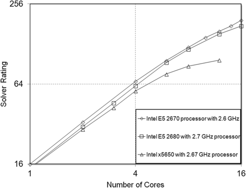
Table 6.11
Core solver rating, core solver speedup, and efficiency details for the problem of flow over an airfoil
| Processes | Machines | Core solver rating | Core solver speedup | Core solver efficiency |
| HP SL230sG8 with Intel Sandy Bridge (16-core dual CPU) with 64 GB RAM per machine, RHEL 6.2 using FDR Infiniband without turbo mode | ||||
| 1 | 1 | 16 | 1 | 100% |
| 2 | 1 | 33 | 2.06 | 103% |
| 4 | 1 | 67 | 4.19 | 105% |
| 6 | 1 | 96 | 6 | 100% |
| 8 | 1 | 121 | 7.56 | 95% |
| 10 | 1 | 143 | 8.94 | 89% |
| 12 | 1 | 159 | 9.94 | 83% |
| 14 | 1 | 175 | 10.94 | 78% |
| 16 | 1 | 193 | 12.06 | 75% |
| Intel Sandy Bridge (16-core dual CPU) with 28 GB RAM | ||||
| 1 | 1 | 14.9 | 1 | 100% |
| 2 | 1 | 30.6 | 2.06 | 103% |
| 3 | 1 | 46.1 | 3.09 | 103% |
| 4 | 1 | 62 | 4.17 | 104% |
| Table Continued | ||||

| Processes | Machines | Core solver rating | Core solver speedup | Core solver efficiency |
| 6 | 1 | 92.9 | 6.24 | 104% |
| 8 | 1 | 116.6 | 7.83 | 98% |
| 12 | 1 | 151.8 | 10.2 | 85% |
| 16 | 1 | 174.9 | 11.75 | 73% |
| Intel Gulftown/Westmere (12-core dual CPU) with 39 GB RAM | ||||
| 1 | 1 | 14.8 | 1 | 100% |
| 2 | 1 | 29.2 | 1.97 | 98% |
| 3 | 1 | 42.4 | 2.86 | 95% |
| 4 | 1 | 56.7 | 3.82 | 96% |
| 6 | 1 | 76.1 | 5.13 | 86% |
| 8 | 1 | 87.3 | 5.88 | 74% |
| 12 | 1 | 96.9 | 6.53 | 54% |

4. OpenFOAM® Benchmarking
Throughout the text we have been discussing commercial codes, mainly ANSYS Fluent. We now focus on open source codes as well. Open source means that you can modify the code according to your need. You may add subroutines, programs, functions, and so on, according to your needs. The most well-known open source code for CFD simulations is OpenFOAM, in which “Open” refers to the open source and “FOAM” stands for Field Operation and Manipulation. The benchmark presented here is for the problem of cavity flow—a famous problem in the CFD community. The case was simulated with the 2.2 version of OpenFOAM.
The following table (Table 6.12) illustrates the conditions under which the problem was simulated.
An Altix system contains processors that are connected by the NUMALINK in a fat-tree topology. The terminology of fat-tree evolves from the fact that branches become thinner as they move from bottom to top; here, network branches become thicker until they reach the master node. Thus, it is like a tree, but inverted.
Like conventional clusters, and in this case as well, each node is fitted into a blade that later fits into an enclosure or chassis; it is also called the individual rack unit (IRU). The IRU is a 10-unit enclosure that contains the necessary components to support the blades, such as power supplies, two router boards (one for every five blades), and an L1 controller. Each IRU can support 10 single-width blades or two double-width blades and eight single-width blades. The IRUs are mounted in a 42-U-high rack; thus, each rack supports up to four IRUs. The Altix ICE X blade enclosure features two 4x DDR Infiniband switch blades.
Table 6.12
Flow conditions for the cavity flow problem
| Reynolds number | 1000 |
| Kinematic viscosity | 0.0001 m2/s |
| Cube dimension | 0.1 × 0.1 × 0.1 m |
| Lid velocity | 1 m/s |
| deltaT | 0.0001 s |
| Number of time steps | 200 |
| Solutions written to disk | 8 |
| Solver for pressure equation | Preconditioned conjugate gradient (PGC) with diagonal incomplete Cholesky smoother (DIC) |
| Decomposition method | Simple |
The process was expedited on an SGI machine by Silicon Graphics, Inc®. The model was an Altix Ice X computer with 1404 nodes, each carrying two eight-core Intel Xeon E5-2670 CPUs and 32 GB memory per node. The interconnect was FDR and FDR-10 Infiniband. For this problem, for larger mesh sizes, the case was split into nodes in multiples of 9. You may consider them to be cores. Here, the nodes are grouped in IRUs of 18 nodes each, where each IRU has two switches connecting 9 × 9 nodes together. It is beneficial to fill these IRUs, with respect to both communication and fragmentation of the job queue.
The simulated cases are shown in Table 6.13. The 27-million mesh size on one node was not run because the RAM was not adequate. On the other hand, smaller mesh sizes are not run on a large number of nodes not because of memory, but because extra time latency in communication causes a drop in parallel performance.
The results of this scaling study are presented as plots indicating speedup and parallel efficiency. All results are based on total analysis time, including all startup overhead.
Speedup and parallel efficiency are calculated with the lowest number of nodes as a reference; i.e., speedup is computed relative to one node for all meshes except the 27-million cell mesh, in which the speedup is relative to two nodes. In Figure 6.13, a trend is evident in that the highest performance is achieved by 27 million cores. The smallest mesh size case does not show linear behavior because efficiency drops with a higher number of processes as a result of intercommunication, as shown in Figure 6.13. Figure 6.14 plots parallel efficiency. The ideal behavior is obviously one corresponding to 100% efficiency. It is normal to obtain efficient results and then to see efficiency drop after a certain number of cores (depending on the problem size and other overheads), just as the speedup drops after a certain number of cores.

Table 6.13
Problem scale span and number of cores
| Nodes | Mesh size | ||||
| 1M | 3.4M | 8M | 15.6M | 27M | |
| 1N (16 cores) | Yes | Yes | Yes | Yes | No |
| 2N (32 cores) | Yes | Yes | Yes | Yes | Yes |
| 4N (64cores) | Yes | Yes | Yes | Yes | Yes |
| 9N (145 cores) | Yes | Yes | Yes | Yes | Yes |
| 18N (288 cores) | Yes | Yes | Yes | Yes | Yes |
| 27N (432 cores) | Yes | Yes | Yes | Yes | Yes |
| 36N (576 cores) | Yes | Yes | Yes | Yes | Yes |
| 72N (1152 cores) | Yes | Yes | Yes | Yes | Yes |
| 144N (2304 cores) | Yes | Yes | Yes | Yes | Yes |
| 288N (4608 cores) | No | No | Yes | Yes | Yes |


5. Case Studies of Some Renowned Clusters
5.1. t-Platforms' Lomonosov HPC
t-Platform is a leading company from Russia in the field of HPC. Germany, the United States, and China are the main competitors in the field of HPC, but the Russians are also on their way to take the lead. This became clear to the world in November 2009, when Lomonosov became the 12th in the Top500 Web site list of the world's largest supercomputers. Figure 6.15 shows the history of supercomputing in Russia. The graph shows the increment in teraflops achieved in the past decade of supercomputing at Moscow State University (MSU). The last three years show that HPC machines in Russia have broken the barrier of teraflops per second by entering into the petaflop range. A number of supercomputing centers working in Russia are shown in Figure 6.16 [3].
5.2. Lomonosov
The Lomonosov is the largest supercomputer in Moscow, Russia, located at MSU. It was named after renowned Russian scientist M.V. Lomonosov [3]. The peak performance of Lomonosov is 420 teraflops and LINPACK measured performance is 350 teraflops. System efficiency is 83%, which is considered the best in the world in terms of the performance of supercomputers. The Lomonosov is based on the T-Blade 1.1i and T-Blade 2T and TB2-TL, which are equipped with GP-GPU nodes. All of the system is in-house except the processors, which are Intel or NVIDIA Tesla, power supply units, and cooling fans. Figure 6.17 shows the hall in which the Lomonosov cluster was installed.


5.2.1. Engineering Infrastructure
The Lomonosov cluster consumes around 1.36 MW of power and has redundant power supply units in case of failure. The uninterruptible power supply (UPS) system is guaranteed to provide sufficient power and cool down the system for the time required to shut down running tasks gracefully and shut the system down appropriately. Two UPS units provide separate power to the two segments of Lomonosov, each with a performance of 200 teraflops.
In addition, in case of power loss, one compute segment can be powered down to allocate more power to the critical computational segment. The specialty of the UPS system is 97%, which is above the conventional 92% used at the industrial level. High efficiency is a must for such huge computational systems.
Another feature of Lomonosov that makes it ubiquitous is its high-scale computational density workload, which draws 65 kW of power per a 42-U, approximately 73.5 in rack. A separate cooling system (Figure 6.18) that occupies an 800 m2 room provides cooling for this massive structure. Because of the long winters in Russia, the system is also cooled by the free outside atmosphere, by cutting off compressors running through water chillers. This helps reduce power consumption for about half the year. The system is also equipped with a fire security system. Within a half second the automatic fire system fills the entire room with a gas, terminating fire without damaging any of the equipment components. The fire is suppressed but it does not lower the concentration of oxygen in the room, and thus it is relatively safe for personnel.
5.2.2. Infrastructure Facts
Preparation for this gigantic mega-structure involves reinforcing floors to accommodate rack cabinets weighing more than 1100 kg each, as well as insulating the data center walls to keep a nominal 50% humidity. Six water tanks are used for the water circulation system, carrying over 31 tons of water to provide necessary cooling. The UPS and the cooling and management subsystems are tightly coupled. The system has a two-stage scenario in which it analyzes the first 3 min of an event to determine whether the power loss was temporary, in which case normal operation can be restored, or whether it is a permanent situation, in which case the system will restart a proper shutdown procedure, creating backups for all running jobs. In the event of external power loss, the entire system takes 10 min to shut down completely. The cooling system consists of an innovative hot–cold air containment system; high-velocity air outlets provide efficient, even air mixed with minimal temperature deviations in the hot aisle zones.
Table 6.14
Key features of the Lomonosov cluster
| Features | Values |
| Peak performance | 420 teraflops/s (heterogeneous nodes) |
| Real performance | 350 teraflops/s |
| LINPACK efficiency | 83% |
| Number of compute nodes | 4446 |
| Number of processors | 8892 |
| Number of processor cores | 35,776 |
| Primary compute nodes | T-Blade 2 |
| Secondary compute nodes | T-Blade 1.1 peak cell S |
| Processor type of primary compute node | Intel Xeon X5570 |
| Processor type of secondary compute node | Intel Xeon X5570, power cell 8i |
| Total RAM installed | 56 TB |
| Primary interconnect | QDR Infiniband |
| Secondary interconnect | 10G ethernet, gigabit ethernet |
| External storage | Up to 1350 TB, t-Platforms ready storage SAN 7998–Lustre |
| Operating system | ClusterX t-Platforms edition |
| Total covered area occupied by system | 252 m2 |
| Power consumption | 1.36 MW |
5.2.3. Key Features
Key features of the Lomonosov cluster are given in Table 6.14. The details consider only the Intel Xeon Westmere series and not NVIDIA GPUs.
5.3. Benchmarking on TB-1.1 Blades
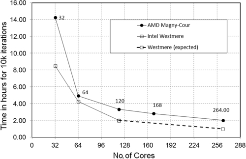
This benchmarking was performed on TB-1.1 blades. These blades are made by MSU HPC team and contained 264 cores in 16 blade enclosures. Thus, each blade contained two processors. The tests were performed in two stages. In the first stage the processors used were AMD Opteron 6174 (Magny-Cour), each with 12 cores, and so 24 cores per blade. In the second stage the processors used were Intel Westmere X5670, each with a hex core, and so 12 cores in a single blade. The performance curves were tested for 3 million and 8 million cells of a CFD problem. The problem consisted of an NACA 0012 aerofoil. These curves were tested for 256 cores of an AMD Magny-Cour processor and a 128 Intel Xeon Westmere processor. Figure 6.19 shows the curve for the 3-million cell problem in ANSYS Fluent and Figure 6.21 shows a plot of the 8-million cell problem in ANSYS Fluent performed with AMD Opteron 6174 (Magny-Cour) processors. Figure 6.20 and Figure 6.22 show the performance curves of Intel Westmere X5670 and a comparison with AMD cores.
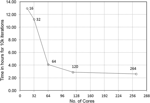
Figure 6.19 Performance results of 3-million mesh size problem run on an Intel Westmare hex core processor.


Figure 6.21 Performance results of an 8-million mesh size problem run on an Intel Westmare hex core processor.
This shows that Intel performs much faster than an AMD processor. An expert from t-Platforms discussed this and said that Intel Xeon performance is much better with AMD Magny-Cour. This is because of the overall clock speed of Intel and AMD. The AMD Magny is 2.2 GHz whereas the Intel Xeon is 2.93 GHz. Overall, for both AMD and Intel it is obvious that for a single problem, as the number of cores increases the time to complete 10,000 iterations decreases until it show no significant decrease with increasing cores. The IST team is thankful to t-Platform for this ultimate support in benchmarking.
5.4. Other t-Platform Clusters
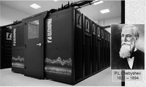
5.4.1. Chebyshev Cluster
The MSU Chebyshev supercomputer (Figure 6.23) with 60 teraflops/s of peak performance was the most powerful computing system in Russia and eastern European countries before Lomonosov. It was named after the Russian mathematician P.L. Chebyshev. The Chebyshev, with 60 teraflops/s of peak performance, was based on 625 blades designed by t-Platform, incorporating 1250 quad-core Intel Xeon E5472 processors. The LINPACK real performance test result was 47.17 teraflops/s or 78.6% peak performance. The MSU Chebyshev supercomputer incorporated the most recent technological findings from the industry and used several in-house developed technologies. Its computing core used the first Russian-developed blade systems, which incorporate 20 quad-core Intel Xeon 3.0 GHz 45 nm processors in a 5-U chassis, providing the highest computing density among all Intel-based blade solutions on the market.
5.4.2. SKIF Ural Supercomputer
The SKIF Ural Supercomputer incorporates advanced technical solutions. It incorporates over 300 up-to-date, 45 nm Intel Hypertown quad-core processors. Along with the SKIF MSU supercomputer, SKIF Ural was the first Russian supercomputer of the time built using the Intel Xeon E5472 processors. This supercomputer is also equipped with advanced engineering software for research involving analysis and modeling. FlowVision is an example and is Russia's indigenous computer product. There are many application areas, the foremost of which is CFD. Others include nanotechnology, optics, deformation and fracture mechanics, 3D modeling and design, and large database processing. In March 2008, SKIF Ural occupied the fourth position in the eighth edition of the Top50 list of the fastest computers in the Commonwealth of Independent States countries.
5.4.3. Shaheen Cluster
The Shaheen cluster consists of a 16-rack IBM Blue Gene/P supercomputer owned and operated by King Abdullah University of Science and Technology (KAUST). Built in partnership with IBM, Shaheen is intended to enable KAUST faculty and partners to research both large- and small-scale projects, from intuition to realization. Shaheen is the largest and most powerful supercomputer in the Middle East. Originally built at IBM’s Thomas J. Watson Research Center in Yorktown Heights, New York, Shaheen was moved to KAUST in mid-2009 [4]. The creator of Shaheen is Majid Alghaslan, KAUST's founding interim chief information officer and the university’s leader in the acquisition, design, and development of the Shaheen supercomputer. Majid was part of the executive founding team for the university and the person who named the machine.
5.4.3.1. System Configuration
Shaheen includes 16 racks of Blue Gene/P, with a peak performance of 222 teraflops. It also contains 128 IBM System X3550 Xeon nodes, with a peak performance of 12 teraflops. The supercomputer contains 65,536 independent processing cores. The Blue Gene/P is technology evolved from Blue Gene/L. Each Blue Gene/P motherboard chip contains four PowerPC 450 processor cores running at 850 MHz. The cores are cache coherent and the chip can operate as a four-way symmetric multiprocessor. The memory subsystem on the chip consists of small private L2 caches, a central shared 8 MB L3 cache, and dual DDR2 memory controllers. The chip also integrates the logic for node-to-node communication, using the same network topologies as Blue Gene/L, but at more than twice the bandwidth. A compute card contains a Blue Gene/P chip with 4 or 4 GB DRAM, comprising a compute node. A single compute node has a peak performance of 13.6 gigaflops. Thirty-two compute cards are plugged into an air-cooled node board. A rack contains 32 node boards (thus, 1024 nodes and 4096 processor cores).
6. Conclusion
This discussion shows how various supercomputer manufacturers market their product by benchmarking. It gives the idea that if users want to make their own cluster or want to hire some vendor, they can easily obtain their desired machine by analyzing standard benchmark curves. However, users must know mesh requirements beforehand. Also, only the speedup curves are important, but also the efficiency, as shown in tabular form for ANSYS Fluent and CFX and in graphical form for OpenFOAM. Budgeting is also important; it is not advisable to buy an expensive machine (such as IBM) if your problems usually run on less than 250 cores. IBM machines are useful for big problem sizes of more than 10 million. This chapter had no rocket science behind it; it was an information guide for establishing an economical and productive HPC cluster.
..................Content has been hidden....................
You can't read the all page of ebook, please click here login for view all page.