CHAPTER 33. Routing Protocols

SOME OF THE MAIN TOPICS IN THIS CHAPTER ARE

---

Basic Types of Routing Protocols 636

Multi-Protocol Label Switching (MPLS) 643

Routers are devices that examine Network layer protocol addresses and make decisions based on those addresses on how best to send a network packet on its way to its destination. Routers can be used in a corporate network to interconnect various LAN segments, to connect to a wide area network (WAN)—for connecting branch offices to the headquarters, other companies or business units for example—or, more commonly, to connect a local network to the Internet.

Routers also play an important part in firewalls, which are covered in Chapter 45, “Firewalls.”

However, to make decisions on the best path a packet needs to take as it travels through the network, a router must keep a table in memory that it can use to locate the destination network for each packet that passes through it. Using the table, the router can find the interface in which the remote network is connected and send it out that interface. Because routers generally are used to connect many different networks, and because networks usually undergo changes frequently, there must be a method for keeping the routing table up-to-date. Network transport protocols (such as TCP/IP) are used to transfer data across a network. Routers use routing protocols to communicate with other routers to exchange information, such as routes or routes that no longer exist.

Chapter 24, “Overview of the TCP/IP Protocol Suite,” not only gives you a detailed overview of TCP/IP, but also contains a great deal of information about address classes, subnet masks, subnetting, and the Classless Interdomain Routing (CIDR), among other basic TCP/IP topics. I strongly recommend that you read Chapter 24 before this one to make it easier for you to comprehend the topics covered here.

For example, suppose that an important router suddenly fails. All other routers that have this router in their routing table need to know this so that they can discover another route, if there is one, that can be used to bypass this failed device. Routing protocols come in all sizes and shapes, but all generally perform the same function: keeping routing tables up-to-date.

Basic Types of Routing Protocols

There are two general types of routing protocols: interior and exterior protocols. Interior protocols perform routing functions for autonomous networks. Exterior routing protocols handle the routing functions between these autonomous networks and glue the Internet together. These routing types are more commonly referred to as Interior Gateway Protocols (IGP) and Exterior Gateway Protocols (EGP). The network you manage for your business is an independent domain that functions internally as a unit. It is an autonomous system within which you can make decisions about which hosts use a particular address and how routing is done. When you connect your network to the Internet, the ISP or other provider manages routers that allow your autonomous system to exchange information with other routers connected to other autonomous systems throughout the Internet.

For the most part, the network administrator is concerned with IGP protocols. The most commonly seen (though not necessarily used) non-proprietary protocols in use today are the Routing Information Protocol (RIP) and Open Shortest Path First (OSPF).

The Routing Information Protocol (RIP)

By default, RIP is the most widely deployed routing protocol for autonomous systems in use today, though that doesn’t mean it’s the best, nor does it mean it’s widely used where it’s deployed. There are newer IGP protocols that give additional functionality, but RIP, due to its low overhead, is still in wide-spread use.

RIP is a distance-vector protocol, which means that it judges the best route to a destination based on a table of information that contains the distance (in hops) and vector (direction) to the destination. A hop is simply another router along the route that the packet will take. There is a limit to the number of hops a packet can take, and this is defined by which routing protocol is used. This value limits the number of routers a packet can pass through before it is dropped. Without this value, it would be possible for a packet to continue to travel through the Internet endlessly if the routers were not correctly configured.

The simplest explanation for how RIP works is that it forwards packets to the router closest to the destination network regardless of link speed or utilization. So if there is a “shortest” way to get to a destination, RIP will forward the packet to the destination network via the shortest hop count it can calculate.

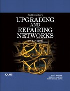
Figure 33.1 shows two company sites that are connected through two links that have routers between them. The user on Workstation A wants to connect to a resource in the remote network that resides on Server A.

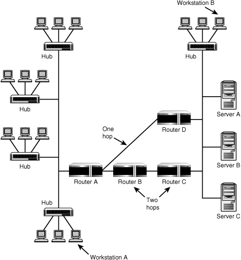
Figure 33.1. RIP decides the best route based on the number of hops between two nodes.

When Router A sees the first packet from workstation A and realizes that it cannot be delivered on the local network, it consults its routing tables to first determine whether it can find a path that will get the data to its destination. If more than one path exists, as it does here, it then makes a decision on which path to take. A simplified version of the routing table information would look like this:

Destination   Next Hop    Metric
Server A    Router D     1
Server A    Router B     2

Router A has two paths it can use to get the packet delivered. The routing table it keeps in memory doesn’t tell it the actual names of the servers, as is shown here. Instead, it uses network addresses. It also doesn’t show every single router through which the packet will pass on its route to its destination. It shows only the next router to send the packet to and the total number of routers through which it will have to pass.

Earlier versions of RIP routing made simple decisions based solely on the metric called a hop count. In this case, RIP would decide to send the packet to Router D, because that route indicates that the packet has to pass through only one additional router to reach its destination network. If it were to route the packet through Router B, it would take two hops.

The number of hops to a destination cannot be infinite. In RIP routing, the maximum number of hops that will be considered is 15. If a destination lies more than 15 hops away from the router, it is considered to be an unreachable destination and the router will not attempt to send a packet. When this happens, the router will send an ICMP Destination Unreachable message back to the source of the network packet. Because RIP is considered an IGP, most packets should never have to pass through more than 15 hops.

For more information about ICMP (the Internet Control Message Protocol), see Chapter 24.

Another situation that needs to be taken into account is that a network administrator can configure a router to use up more than a single hop or metric value. Because of this, it is possible that a network packet may be dropped before it passes through 15 actual routers.

As simple and straightforward as this might seem, it might not be the best route to take. One of the problems that RIP routing has is that it never takes into consideration the bandwidth of the route. The path from Router A to Router C might be made up of high-speed T1 links, and the line between Router A and Router D might be a slower connection. For small simple packets, such as an email delivery, this might not make a great deal of difference to the end user, because a few seconds or a minute or two won’t make much difference for this type of application. For a large amount of traffic, though, this can make a significant difference. Routing a lot of traffic over slow links can significantly impact performance.

Another problem with RIP is that it doesn’t load balance. If a lot of users are trying to get to the remote system, it will not use both of the available routes and divide up the traffic. RIP continues to select what it considers the best route and just sends the packets on their way.

You can also manipulate the metric value used in the routing table to make it appear that one route—usually a slower link—is farther away than a faster route simply by modifying the routing table to change the hop count of the slow route to a number larger than that of the faster route link. Thus, although a faster link might actually send packets through more routers than the slower link, you can “fool” RIP into using the faster link.

Updating Routers

RIP routers periodically exchange data with each other (through the User Datagram Protocol, or UDP, using port 520) so that each router can maintain a table of routing information that is more or less up-to-date. In earlier versions of RIP, a router would broadcast its entire routing table. Newer versions allow a router to send only changes or to respond to routing requests from other routers (called triggered RIP updates).

The format of the RIP message for version 1 appears in Figure 33.2. For version 1 of the protocol, the largest RIP message that can be sent in a UDP datagram is 504 bytes. When you combine this with the 8-byte UDP header, the maximum size of the datagram is 512 bytes.

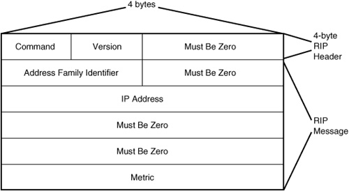
Figure 33.2. The format of the RIP message for version 1 of the protocol.

In Figure 33.2, the portion following the first 4 bytes can be repeated as many as 25 times, depending on the number of routes that are being sent in a single message. The fields labeled Must Be Zero should contain all zero bits. The first field, Command, can have the following values, which indicate the purpose of the message:

1 Request—This message requests that the recipient of the message send all or part of its routing table to the sender of this message.

2 Response—This message is a response to a request, and contains all or part of the sender’s routing table to the requestor. Additionally, this message can be sent as an update message that does not correspond with any particular request.

3 Traceon—This is an obsolete command that should be ignored.

4 Traceoff—This is an obsolete command that should be ignored.

5—This is a value reserved by Sun Microsystems for its own use. Implementations of RIP might or might not ignore this type of command.

The Version field denotes the version of the RIP protocol. For version 1 this field contains, of course, a value of 1. The Address Family Identifier field was defined in RFC 1058, but only one address type (the IP address) was defined, and the value for this field should be 2. The IP Address field is 4 bytes long and is used to store a network address or a host address. For most request messages, this value is set to the default route of 0.0.0.0.

The final field is used to store the hop count, or metric, for the route. This field can contain a value ranging from 1 to 16. A value of 16 indicates that the destination is unreachable, or to put it in other words, “you can’t get there from here.”

Because RIP version 1 was created before Classless Interdomain Routing (CIDR), and before the concept of subnetting was introduced, there is no subnet field in the message. Because of this, a RIP version 1 router must determine the network ID by examining the first 3 bits of the IP address, which determine to which class (A, B, or C) the network address belongs. From this it can apply the appropriate subnet mask for the class. If the address does not fall into one of these classes, the router will use the subnet mask associated with the interface on which it received the message and apply it to the address to determine whether it is a valid network address. If that subnet mask does not match up to create a network address, the mask of all 1s (255.255.255.255) is applied, and the address is assumed to be a host address instead of a network address.

The message traffic generated by RIP routers can be significant in a large network. RIP routers update their routing tables every 30 seconds by requesting information from neighboring routers. They also announce their existence every 180 seconds—hey, you have to allow for network latency and other network problems, so the 180 seconds value was chosen to give more than 30 seconds for another router to respond when changes are being sent or received. If a router fails to announce itself within this time, other routers will consider it to be down and will modify their routing tables. The router itself might have been taken offline by the network administrator, or it could have simply gone offline due to hardware failure. It’s also quite possible that the network link between the router and the rest of the network has been broken. The thing to remember is that RIP routers dynamically update routing tables so that packets don’t get sent out into the ether and just disappear!

RIP Version 2

Although other protocols, such as OSPF (described later in this chapter) were developed after the original version of RIP and contain more features, you might wonder why RIP version 2 was developed. The reasons are simple: RIP has a large installed base, and it’s easy to implement and configure. And, for small to medium-sized networks, you don’t necessarily need a more complex routing protocol when RIP will do the job just as well.

Version 2 of the protocol uses a slightly different message format, as shown in Figure 33.3.

Figure 33.3. Format of the RIP message for version 2 of the protocol.

As you can see, the message format is the same size, but some of the fields that were previously reserved for all zeros have been put to use in version 2 of the protocol. Specifically, they contain Route Tag, Subnet Mask, and Next Hop fields.

The Route Tag field is an administrative field used to mark certain routes. This field was introduced in RFC 1723 so that routers that support multiple routing protocols could distinguish between RIP-based routes and routes imported from other routing protocols. The Subnet Mask field is used to implicitly store a subnet mask associated with the IP address field so that the router does not have to try to determine the network or host address. Applying the mask can yield this result.

The Next Hop field is used to indicate the IP address to send packets for the destination advertised by this route message. If this field is not set to 0.0.0.0, the address in this Next Hop field must be reachable on the logical subnet from which the routing advertisement originates.

Disadvantages of RIP

RIP is a good routing protocol to use in small networks, but it doesn’t scale very well to very large networks. It became quite popular early on because it was distributed as part of the Berkeley version of Unix, in the form of the routed daemon. The following are the major disadvantages of RIP:

The broadcast messages used to update routing tables can use a significant amount of network bandwidth.

There is no general method to prevent routing loops from occurring.

For larger networks, 15 hops might not be a large enough figure for determining whether a destination is unreachable.

Update messages propagate across the network slowly from one router to the next, hop by hop (called slow convergence), so inconsistencies in routing tables can cause a router to send a packet using a route that no longer exists.

Depending on the version of RIP you use (V1 or V2), you might not be able to support CIDR and VLSMs.

OSPF (Open Shortest Path First)

RIP is a vector-distance protocol, whereas OSPF uses a link-state algorithm. OSPF routers maintain a routing table in memory just as RIP routers do, but instead of sending out the entire routing table in a broadcast every 30 seconds, OSPF routers exchange link-state information every 30 minutes and keep each other updated every 10 seconds with small Link State Advertisements (LSAs), also called hello packets.

The Open Shortest Path First (OSPF) routing protocol (version 2) is defined in RFC 2328, “OSPF Version 2.”

OSPF was developed by the Internet Engineering Task Force and was meant to solve most of the problems associated with RIP. Instead of using a simple hop count metric, OSPF also takes into consideration other cost metrics, such as the speed of a route, the traffic on the route, and the reliability of the route. Also, OSPF does not suffer from the 15-hop limitation that RIP employs. You can place as many routers between end nodes as required by your network topology. Another difference between RIP and OSPF is that OSPF provided for the use of subnet masks at a time when version 1 of RIP did not.

Although OSPF functions more efficiently than RIP, in a large network the exchange of information between many routers still can consume a lot of bandwidth. The time spent recalculating routes can add to network delay. Because of this, OSPF incorporates a concept called an area, which is used to divide up the network. Routers within a specific area (usually a geographical area, such as a building or campus environment) exchange LSAs about routing information within their area.

The Link State Database (LSDB) and Areas

Each router maintains a Link State Database (LSDB), in which it stores the information it receives through LSAs from neighboring routers. Thus, over time, each OSPF router essentially has an LSDB that is identical to other routers with which it communicates. Each router is assigned a router ID, which is simply a 32-bit dotted decimal number that is unique within the autonomous network. This number is used to identify LSAs in the LSDB. This is not to be confused with the actual IP addresses of the router’s interfaces, but is merely a number used to identify the router to other routers. However, most implementations of OSPF will use either the largest or the smallest IP address of a router’s interfaces for this value. Because IP addresses are unique within the autonomous network, Router IDs also will be unique.

A router that is used to connect these areas with a backbone of other routers is called a border router. A hierarchy of routing information is built using this method so that every router does not have to maintain a huge database showing the route to every possible destination. Instead, a border router will advertise a range of addresses that exist within its area instead of each address. Other border routers store this information and therefore have to process only a portion of an address instead of the entire address when making a routing decision. Border routers store this higher level of routing information and the information for routes in their area.

In Figure 33.4, you can see a network that has four major areas, each of which has routers that maintain a database of information about its specific area. These routers exchange information with each other that keeps them updated. Each area has a border router that is part of the area and also part of the backbone area. These border routers exchange summary information about their respective areas with other border routers that are part of the backbone area.

Figure 33.4. OSPF routers are responsible for their areas.

OSPF has the drawback of administrative overhead. Also, low-end routers might not be capable of coping with the amount of information a border router needs to manage.

OSPF Route Calculations

I’ll leave the exact explanation of how OSPF calculates the best route to the mathematicians. However, for those who are interested, the algorithm used is called the Dijkstra algorithm, and it is used to create a shortest path tree (SPF tree) for each router. This tree contains information that is valid only from a particular router’s point of view. That is, each router builds its own tree, with itself as the root of the tree, while the branches of the tree are other routers that participate in the network. Thus, each OSPF router has a different tree than other routers in the network. From this tree, the router can build a routing table that is used for the actual lookup that is performed when deciding which interface a packet should be sent out on.

Multi-Protocol Label Switching (MPLS)

Today the division between routers and switches is a fine line. Whereas switches were initially designed to help segment a LAN into multiple collision domains, and thereby allow you to extend the reach of a particular LAN topology, switches have moved higher up the networking ladder. When switching is used in a LAN to connect individual client and server computers, the process is known as microsegmentation, because the collision domain has been reduced to just the switch and the computer attached to a port. Switches at this level generally work using the hardware (MAC) addresses of the attached computers.

Layer 3 switching moves switching up the ladder by one rung by switching network frames based on the OSI Network layer address—an IP address, for example. But wait, that’s what a router does, isn’t it? Of course. A layer 3 switch is basically a router, but it implements most of its functions in application-specific integrated chips (ASICS) and performs its packet processing much faster than does a traditional router, which uses a microprocessor (much like a computer CPU) for this function.

Details on layer 3 switching can be found in Chapter 8, “Network Switches.”

When you get to the top of the ladder, where large volumes of data need to be routed through a large corporate network—or the Internet, for that matter—even the fastest traditional routers or layer 3 switches easily can become bogged down by the volume of traffic. Because of this, the core of a large network traditionally has been built using ATM or Frame Relay switches, and IP traffic is sent over these switched networks.

To speed up the processing of routing packets at high-volume rates, a newer technology has been developing over the past few years and goes by the name of Multi-Protocol Label Switching (MPLS). MPLS is covered in the next section.

Combining Routing and Switching

Traditional routers have a large amount of overhead processing they must perform to get a packet to its destination. Each router along the packet’s path must open up and examine the layer 3 header information before it can decide on which port to output the packet to send it to its next hop on its journey. If a packet passes through more than just a few routers, that’s a lot of processing time. Remember that IP is a connectionless protocol. Decisions must be made about a packet’s travel plans at each stage of its journey through the network. The solution to this problem lies in newer technology—high-speed switching. Specifically, Multi-Protocol Label Switching, which is discussed in the next section, combines the best of routing techniques with switching techniques.

When you look at concepts such as ATM or Frame Relay, which are connection-oriented protocols, this isn’t the case. Instead, virtual circuits (either permanent or switched) are set up to connect to endpoints of a communication path so that all cells (as in the case of ATM) or frames (as in the case of Frame Relay) usually take the same path through the switched network.

For more information about ATM and Frame Relay and how these connection-oriented switched networks function, see Chapter 15, “Dedicated Connections.”

Adding a Label

MPLS is a method that takes the best of both worlds and creates a concept that allows IP packets to travel through the network as if IP were a connection-oriented protocol (which it isn’t). Using special routers called Label Switching Routers (LSRs) does this. These routers connect a traditional IP network to an MPLS network. A packet enters the MPLS network through an ingress LSR, which attaches a label to the packet, and exits the MPLS switched network through an egress LSR. The ingress LSR is the router that performs the necessary processing to determine the path a packet will need to take through the switched network. This can be done using traditional routing protocols such as OSPF. The path is identified by the label that the ingress router attaches to the packet. As you can see, the ingress router must perform the traditional role that a router fills. It must perform a lookup in the routing table and decide to which network the packet needs to be sent for eventual delivery to the host computer.

However, as the packet passes through the switched network, it is only necessary for the switch to take a quick look at the label to make a decision on which port to output the packet. A table called the Label Information Base (LIB) is used in a manner similar to a routing table to determine the correct port based on the packet’s label information. The switch doesn’t perform IP header processing, looking at the IP address, the TTL value, and so on. It just spends a small amount of time doing a lookup of the label in the table and outputting the packet on the correct port.

When the packet reaches the egress LSR, the label is removed by the router, and then the IP packet is processed in the normal manner by traditional routers on the destination network.

If this sounds like a simple concept, that’s because it is. MPLS still is in the development stages, so you’ll find that different vendors implement it in different ways. Several Internet draft documents attempt to create a standard for MPLS. Other features, such as Quality of Service (QoS) and traffic management techniques, are being developed to make MPLS a long-term solution.

Using Frame Relay and ATM with MPLS

One of the best features about the current design of MPLS is that it separates the label-switching concept from the underlying technology. That is, you don’t have to build special switches that are meant for just MPLS networks. MPLS doesn’t care what the underlying transport is. It is concerned only with setting up a path and reducing the amount of processing a packet takes as it travels through the circuit.

Because of this, it’s a simple matter for an ATM or Frame Relay switch vendor to reprogram or upgrade its product line to use MPLS. For ATM switches, the VPI (virtual path identifier) and VCI (virtual channel identifier) fields in the ATM cell are used for the Label field. In Frame Relay switches, an extra field is added to the IP header to store the label. However, don’t get confused and think that an MPLS network is an ATM network or a Frame Relay network. These switches must be reprogrammed to understand the label concept. It’s even possible, for example, for an ATM switch to switch both ATM and MPLS traffic at the same time. By allowing for the continued use of existing equipment (and these switches are not inexpensive items), large ISPs or network providers can leverage their current investment, while preparing to install newer MPLS equipment when the standards evolve to a stage that makes it a good investment.

For the long term it’s most likely that MPLS will be implemented using technology similar to Frame Relay instead of ATM. This is because of the small cell size of the ATM cell (53 bytes) combined with a high overhead (the 5-byte cell header). In a small network with little traffic, this 5-byte cell header seems insignificant. However, when you scale this to large bandwidth network pipes, this amount of overhead consumes a large amount of bandwidth given the small amount of data carried in the 53-byte cell. Thus, variable-length frames are most likely to become the basis for MPLS networks in the next few years.