
Chapter 8
System-Level Specification
So far we have presented the four main enabling technologies of the LTE (Long Term Evolution) standard individually: OFDM (Orthogonal Frequency Division Multiplexing) multicarrier transmission, MIMO (Multiple Input Multiple Output) multi-antenna techniques, channel coding based on turbo coders, and link adaptations. OFDM in downlink and its single-carrier counterpart SC-FDM (Single-Carrier Frequency Division Multiplexing) in uplink provide the backbone of the LTE transmission strategy. As examined in Chapter 7, adaptive modulation and coding provide superior spectral efficiency. Arguably the defining feature that sets LTE apart from the previous standards is the incorporation of various types of MIMO technique. At any given time, the operating mode of the LTE downlink transceiver system is uniquely defined by one of the nine MIMO multi-antenna techniques specified in the LTE standard. As a result, when evaluating the performance of an LTE system we should pay special attention to the type of MIMO technique used and the corresponding channel operating conditions.
In this chapter we will put together a simulation model for the PHY (Physical Layer) of the LTE standard. So far, our pedagogic step-by-step approach has demanded that we focus on a single transmission mode at a time. In this chapter, we develop a simulation model that incorporates multiple transmission modes in both the transmitter and the receiver. We also evaluate various aspects related to the performance of the system.
We will highlight both the common set of processing performed in multiple modes and the specific features used in any particular transmission mode. To stay true to our focus on examining user-plane processing and single-carrier operations, our simulation model will include the first four transmission modes of the LTE standard. Then we will evaluate the performance of the system under changing operating conditions; this includes examining system quality and throughput when using different types of MIMO mode, channel model, channel estimation technique, and MIMO receiver algorithm. Finally, we will create a Simulink model for our LTE PHY system. We will show how easy it is to incorporate the MATLAB® algorithms developed throughout this book as distinct blocks within the Simulink model. Expressing the design as a Simulink model has the added benefit of having Simulink as the simulation testbench. Instead of developing MATLAB scripts to perform various operations in the loop and call the algorithms and visualization functions iteratively, we will use the Simulink model to perform these tasks. In the final section of this chapter, we will undertake a qualitative assessment of the performance of our LTE model. We will use the LTE Simulink model to stream audio signals as the inputs to the downlink transmitter and will listen to and assess the quality of the recovered voice at the receiver after a certain amount of processing delay.
8.1 System Model
In this section, we compose a system model for the PHY of the LTE standard by integrating various enabling technologies. The system model is composed of a transmitter, a channel model, and a receiver. The processing chain in the transmitter is specified in detail by the standard. The standard also specifies various channel models for performance evaluations. The receiver operations, however, are not specified, which provides the opportunity for various system designers to distinguish their implementation with distinct performance profiles.
Figure 8.1 illustrates the overall structure of the LTE downlink transceiver. The payload bits provided by the transport channel are processed by the transmitter. The transmitter output is composed of a sequence of the symbols transmitted on various available transmit antennas. The channel operates on the transmitted symbols of multiple transmit antennas to produce the set of received symbols arriving at each of the receive antennas. The receiver operates on the received symbols. By implementing various strategies aimed at inverting the operations of the transmitter, the receiver generates its best estimate of the transmitted payload bits.
Figure 8.1 LTE downlink PHY transceiver model

8.1.1 Transmitter Model
In the transmitter, the signal processing chain is applied to the payload bits provided by the transport channel. The processing depends on the transmission mode, defined by the downlink scheduler. The transmission mode manifests itself as the choice of MIMO technique used at any given subframe. In this book, we have focused on the first four of the nine transmission modes used in the LTE standard. Figure 8.2 illustrates the processing chain in the downlink transmitter.
Figure 8.2 LTE downlink system model: transmission modes 1–4, transmitter operations

In each subframe, the scheduler selects one of the four transmission modes: the first implements a single-antenna transmission and can be referred to as a SIMO (Single Input Multiple Output) mode. The second employs transmit diversity, where redundant information is transmitted on multiple antennas to boost the overall link reliability. The third and fourth both employ spatial-multiplexing MIMO techniques to boost data rates. The third mode uses open-loop spatial multiplexing and is intended for transmission in high-mobility scenarios, while the fourth uses closed-loop spatial multiplexing intended mostly for low-mobility scenarios and is responsible for the highest data rates achievable by the LTE standard.
In each transmission mode, we go through a series of operations that are a combination of Downlink Shared Channel (DLSCH) and Downlink Shared Physical Channel (PDSCH) processing steps. Many of the PDSCH and DLSCH operations are common to all transmission modes. The distinctive MIMO-specific operations in each mode are the elements that set it apart from the others.
Common operations include the transport block CRC (Cyclic Redundancy Check) attachment, code-block segmentation and attachment, turbo coding, rate matching, and code-block concatenation to generate codewords. The codewords constitute the inputs of the PDSCH processing chain. The LTE downlink specification supports one or two codewords. To make the MATLAB algorithm easier to read, we show here only the closed-loop spatial-multiplexing case (mode 4) with either one or two codewords. In the PDSCH, common operations are scrambling, modulation of scrambled bits to generate modulation symbols, mapping of modulation symbols to resource elements, and generation of OFDM signal for transmission on each antenna port.
Different transmission modes are differentiated by their respective MIMO operations. In the case of the SIMO mode, no particular MIMO operations are performed and the modulation symbols map directly to the resource grid. In the second mode, transmit diversity is applied to the modulated symbols. This operation can be viewed as a combined form of layer mapping and precoding. A transmit-diversity encoder subdivides the modulated stream into different substreams intended for different transmit antennas. This is analogous to a layer-mapping operation. Transmit diversity also assigns to each transmit antenna orthogonally transformed substreams that can be regarded as a special type of precoding.
In spatial multiplexing modes 3 and 4, we explicitly perform layer mapping and precoding operations on the modulated symbols. The outputs of MIMO operations are then placed as resource elements in the resource grid. In mode 3, the open-loop precoding implies that the precoder matrix is independently generated at the transmitter and the receiver and does not require transmission of any precoding data. In closed-loop spatial multiplexing, we use either a constant precoder throughout the simulation or a closed-loop feedback in the receiver to signal which precoder matrix index needs to be transmitted in the following subframe.
8.1.2 MATLAB Model for a Transmitter Model
The following MATLAB function shows the LTE downlink transmitter operations for the transmission mode used in any given subframe. It can be viewed as a combination of the SIMO, transmit-diversity, open-loop, and closed-loop spatial-multiplexing transmitters developed in the previous chapters. The function takes as input the subframe number (nS) and the three parameter structures (prmLTEDLSCH, prmLTEPDSCH, prmMdl). As the function is called in each subframe, it first generates the transport-block payload bits and then proceeds with the common DLSCH and PDSCH operations. Using a MATLAB switch-case statement, it then performs MIMO operations specific to the selected transmitted mode. The MIMO output symbols and the cell-specific resource symbols (pilots) generated are then mapped into the resource grid. The OFDM transmission operations applied to the resource grid finally generate the output transmitted symbols (txSig).
function [txSig, csr_ref] = commlteMIMO_Tx(nS,  dataIn, prmLTEDLSCH, prmLTEPDSCH,
prmMdl)
%#codegen
%  Generate payload
dataIn1 = genPayload(nS,  prmLTEDLSCH.TBLenVec);
% Transport block CRC generation
tbCrcOut1 =CRCgenerator(dataIn1);
% Channel coding includes - CB segmentation, turbo coding, rate matching,
% bit selection, CB concatenation - per codeword
[data1, Kplus1, C1] = lteTbChannelCoding(tbCrcOut1, nS, prmLTEDLSCH,
prmLTEPDSCH);
%Scramble codeword
scramOut = lteScramble(data1, nS, 0, prmLTEPDSCH.maxG);
% Modulate
modOut = Modulator(scramOut, prmLTEPDSCH.modType);
%%%%%%%%%%%%%%%%%%%%%%%
% MIMO transmitter based on the mode
%%%%%%%%%%%%%%%%%%%%%%%
numTx=prmLTEPDSCH.numTx;
dataIn= dataIn1;
Kplus=Kplus1;
C=C1;
Wn=complex(ones(numTx,numTx));
switch prmLTEPDSCH.txMode
    case 1  % Mode 1: Single-antenna (SIMO mode)
        PrecodeOut =modOut;
    case 2   % Mode 2: Transmit diversity
        % TD with SFBC
        PrecodeOut = TDEncode(modOut(:,1),prmLTEPDSCH.numTx);
    case 3   % Mode 3: Open-loop Spatial multiplexing
        LayerMapOut = LayerMapper(modOut, [], prmLTEPDSCH);
        % Precoding
        PrecodeOut = SpatialMuxPrecoderOpenLoop(LayerMapOut, prmLTEPDSCH);
    case 4    % Mode 4: Closed-loop Spatial multiplexing
        if  prmLTEPDSCH.numCodeWords==1
            % Layer mapping
            LayerMapOut = LayerMapper(modOut, [], prmLTEPDSCH);
        else
            dataIn2 = genPayload(nS,  prmLTEDLSCH.TBLenVec);
            tbCrcOut2 =CRCgenerator(dataIn2);
            [data2, Kplus2, C2] = lteTbChannelCoding(tbCrcOut2, nS, prmLTEDLSCH,
prmLTEPDSCH);
            scramOut2 = lteScramble(data2, nS, 0, prmLTEPDSCH.maxG);
            modOut2 = Modulator(scramOut2, prmLTEPDSCH.modType);
            % Layer mapping
            LayerMapOut = LayerMapper(modOut, modOut2, prmLTEPDSCH);
            dataIn= [dataIn1;dataIn2];
            Kplus=[Kplus1;Kplus2];
            C=[C1; C2];
        end
        % Precoding
        usedCbIdx = prmMdl.cbIdx;
        [PrecodeOut, Wn] = SpatialMuxPrecoder(LayerMapOut, prmLTEPDSCH, usedCbIdx);
end
% Generate Cell-Specific Reference (CSR) signals
numTx=prmLTEPDSCH.numTx;
csr = CSRgenerator(nS, numTx);
csr_ref=complex(zeros(2*prmLTEPDSCH.Nrb, 4, numTx));
for m=1:numTx
    csr_pre=csr(1:2*prmLTEPDSCH.Nrb,:,:,m);
    csr_ref(:,:,m)=reshape(csr_pre,2*prmLTEPDSCH.Nrb,4);
end
% Resource grid filling
txGrid = REmapper_mTx(PrecodeOut, csr_ref, nS, prmLTEPDSCH);
% OFDM transmitter
txSig = OFDMTx(txGrid, prmLTEPDSCH);
8.1.3 Channel Model
Channel modeling is performed by combining a MIMO fading channel with an AWGN (Additive White Gaussian Noise) channel. MIMO channels specify the relationships between signals transmitted over multiple transmit antennas and signals received at multiple receive antennas. Typical parameters of MIMO channels include the antenna configurations, multipath delay profiles, maximum Doppler shifts, and spatial correlation levels within the antennas in both the transmitter side and the receiver side. The AWGN channel is usually specified using the SNR (Signal-to-Noise Ratio) value or the noise variance. Figure 8.3 illustrates the operations performed within a fading-channel model, showing an example in which a 4 × 4 MIMO channel connects a single path of the transmitted signals from four transmit antennas to four receive antennas. The uncorrelated white Gaussian noise is then added to each MIMO received signal to produce the channel-modeling output signal.
Figure 8.3 LTE downlink system model: channel model per path

8.1.4 MATLAB Model for a Channel Model
The following MATLAB function shows how channel modeling is performed by combining a multipath MIMO fading channel with an AWGN channel. First, by calling the MIMOFadingChan function, we generate the faded version of the transmitted signal (rxFade) and the corresponding channel matrix (chPathG). The MIMO fading channel computes the faded signal as a linear combination of multiple transmit antennas. As a result, the output signal (rxFade) may not have an average power (signal variance) of one. To compute the noise variance needed to execute the AWGNChannel function, we need to first compute the signal variance (sigPow) and then derive the noise variance as the difference between the signal power and the SNR value in dB.
function [rxSig, chPathG, nVar]  = commlteMIMO_Ch(txSig, prmLTEPDSCH,  prmMdl )
%#codegen
snrdB = prmMdl.snrdB;
% MIMO Fading channel
[rxFade, chPathG] = MIMOFadingChan(txSig, prmLTEPDSCH, prmMdl);
% Add AWG noise
sigPow = 10*log10(var(rxFade));
nVar = 10.^(0.1.*(sigPow-snrdB));
rxSig =  AWGNChannel(rxFade, nVar);
8.1.5 Receiver Model
In the receiver, the signal processing chain is applied to the received symbols following channel modeling. At the receiver, essentially the inverse operations to those of the transmitter are performed in order to obtain a best estimate of the transmitted payload bits. Figure 8.4 illustrates the processing chain in the downlink receiver.
Figure 8.4 LTE downlink system model: transmission modes 1–4, receiver operations

At the receiver, the first few operations are independent of the transmission mode. These include the OFDM receiver, resource element demapping, and Cell-Specific Reference (CSR) signal extraction. Following these common operations, we reconstruct the resource grid at the receiver and extract the user data and the CSR signal from it. Based on the received CSR signals, we then estimate the channel response matrices in each subframe. The channel estimation can be based on multiple algorithms: the ideal estimation algorithm exploits a complete knowledge of channel-state information, while other algorithms are based on various forms of interpolation and averaging.
At this point, we perform the MIMO detection operations based on the scheduled transmission mode in order to recover the best estimates of the modulated symbols. In SIMO mode, receiver detection is same as frequency-domain equalization. In transmit-diversity mode, the transmit-diversity combiner operation is performed. In spatial-multiplexing modes, the MIMO receiver operations are performed in order to solve the MIMO equation for each received symbol given the estimated channel matrix and then different substreams are explicitly mapped back to a single modulated stream using the layer-demapping operation.
The difference between the open-loop (mode 3) and the closed-loop (mode 4) MIMO receivers relates to the precoder matrix. The open-loop algorithm uses different precoder matrix values for different predetection received symbols, whereas the closed-loop algorithm uses a common precoder matrix for all received symbols. After we obtain the best estimates of the modulated symbols, we perform demodulation, descrambling, channel-decoding, and CRC-detection operations in order to obtain best estimates of the payload bits at the receiver. Where a sphere decoder is used as part of the MIMO receiver algorithm, we bypass the demodulation as it is included within the sphere-decoding algorithm. The operations following MIMO detection are repeated according to the number of transmitted codewords.
8.1.6 MATLAB Model for a Receiver Model
The following MATLAB function shows the LTE downlink receiver operations for a given transmission mode used in any subframe. The function takes as input the subframe number (nS), the OFDM signal processed by the channel (rxSig), an estimate of the noise variance per received channel (nVar), the channel-path gain matrices (chPathG), the transmitted cell-specific reference signals (csr_ref), and the three parameter structures (prmLTEDLSCH, prmLTEPDSCH, prmMdl). It generates as its output a best estimate of the transport-block payload bits (dataOut). As described in the last section, the function first performs common OFDM receiver and demapping operations in order to recover the resource grid and estimate the channel response and then, using a MATLAB switch-case statement, performs MIMO receiver operations specific to the selected transmitted mode (represented by the prmLTEPDSCH.txMode variable). Finally, by performing common demodulation, descrambling, channel decoding, and CRC-detection operations, the function computes its output signal.
function dataOut = commlteMIMO_Rx(nS, rxSig, chPathG, nVar, csr_ref,  prmLTEDLSCH,
prmLTEPDSCH, prmMdl)
%#codegen
% OFDM Rx
rxGrid = OFDMRx(rxSig, prmLTEPDSCH);
% updated for numLayers -> numTx
[dataRx, csrRx, idx_data] = REdemapper_mTx(rxGrid, nS, prmLTEPDSCH);
% MIMO channel estimation
if prmMdl.chEstOn
    chEst = ChanEstimate_mTx(prmLTEPDSCH, csrRx,  csr_ref, prmMdl.chEstOn);
    hD     = ExtChResponse(chEst, idx_data, prmLTEPDSCH);
else
    idealChEst = IdChEst(prmLTEPDSCH, prmMdl, chPathG);
    hD =  ExtChResponse(idealChEst, idx_data, prmLTEPDSCH);
end
%%%%%%%%%%%%%%%%%%%%%%%%%%%%
% MIMO Receiver based on the mode
%%%%%%%%%%%%%%%%%%%%%%%%%%%%
dataOut=false(size(dataIn));
switch prmLTEPDSCH.txMode
    case 1
        % Based on Maximum-Combining Ratio (MCR)
        yRec = Equalizer_simo(dataRx, hD, max(nVar), prmLTEPDSCH.Eqmode);
        cwOut = yRec;
    case 2
        % Based on Transmit Diversity  with SFBC combiner
        yRec = TDCombine(dataRx, hD, prmLTEPDSCH.numTx, prmLTEPDSCH.numRx);
        cwOut = yRec;
    case 3
        yRec = MIMOReceiver_OpenLoop(dataRx, hD, prmLTEPDSCH, nVar);
        % Demap received codeword(s)
        [cwOut, ˜] = LayerDemapper(yRec, prmLTEPDSCH);
    case 4
        % Based on Spatial Multiplexing
        yRec = MIMOReceiver(dataRx, hD, prmLTEPDSCH, nVar, Wn);
        % Demap received codeword(s)
        [cwOut1, cwOut2] = LayerDemapper(yRec, prmLTEPDSCH);
        if  prmLTEPDSCH.numCodeWords==1
            cwOut = cwOut1;
        else
            cwOut = [cwOut1, cwOut2];
        end
end
% Codeword processing
Len=numel(dataOut)/prmLTEPDSCH.numCodeWords;
index=1:Len;
for n = 1:prmLTEPDSCH.numCodeWords
    % Demodulation
    if prmLTEPDSCH.Eqmode == 3
        % not necessary in case of Sphere Decoding
        demodOut = cwOut(:,n);
    else
        % Demodulate
        demodOut = DemodulatorSoft(cwOut(:,n), prmLTEPDSCH.modType, max(nVar));
    end
    % Descramble received codeword
    rxCW =  Descramble(demodOut, nS, 0, prmLTEPDSCH.maxG);
    % Channel decoding includes CB segmentation, turbo decoding, rate dematching
    [decTbData, ˜,˜] = TbChannelDecoding(nS, rxCW, Kplus(n), C(n),  prmLT-
EDLSCH, prmLTEPDSCH);
    % Transport block CRC detection
    [dataOut(index), ˜] = CRCdetector(decTbData);
    index = index +Len;
end
8.2 System Model in MATLAB
In this section, we showcase the MATLAB testbench (commlteSystem) that represents the system model for the PHY of the LTE standard. First it calls the initialization function (commlteSystem_initialize) to set all the relevant parameter structures (prmLTEDLSCH, prmLTEPDSCH, prmMdl). Then it uses a while loop to perform subframe processing by calling the MIMO transceiver function composed of the transmitter (commlteSystem_Tx), the channel model (commlteSystem_Channel), and the receiver (commlteSystem_Rx). Finally, it updates the Bit Error Rate (BER) and calls the visualization function to illustrate the channel response and modulation constellation before and after equalization. By comparing the transmitted and received bits, we can then compute various measures of performance based on the simulation parameters.
% Script for LTE (mode 1 to 4, downlink transmission)
%
% Single or double codeword transmission for mode 4
%
clear functions
%%
commlteSystem_params;
[prmLTEPDSCH, prmLTEDLSCH, prmMdl] = commlteSystem_initialize(txMode, …
    chanBW, contReg, modType, Eqmode,numTx, numRx,cRate,maxIter, fullDecode,
chanMdl, Doppler, corrLvl, …
    chEstOn, numCodeWords, enPMIfback, cbIdx);
clear txMode chanBW contReg modType Eqmode numTx numRx cRate maxIter
fullDecode chanMdl Doppler corrLvl chEstOn numCodeWords enPMIfback cbIdx
%%
disp('Simulating the LTE Downlink - Modes 1 to 4');
zReport_data_rate_average(prmLTEPDSCH, prmLTEDLSCH);
hPBer = comm.ErrorRate;
%% Simulation loop
tic;
SubFrame =0;
nS = 0; % Slot number, one of [0:2:18]
Measures = zeros(3,1); %initialize BER output
while (Measures(3) < maxNumBits) && (Measures(2) < maxNumErrs)
    %% Transmitter
    [txSig, csr, dataIn] = commlteSystem_Tx(nS, prmLTEDLSCH, prmLTEPDSCH, prmMdl);
     %% Channel model
     [rxSig, chPathG, ˜]  = commlteSystem_Channel(txSig, snrdB, prmLTEPDSCH,  prmMdl );
     %% Receiver
     nVar=(10.^(0.1.*(-snrdB)))*ones(1,size(rxSig,2));
     [dataOut, dataRx, yRec] = commlteSystem_Rx(nS, csr, rxSig, chPathG, nVar, …
         prmLTEDLSCH, prmLTEPDSCH, prmMdl);
    %% Calculate  bit errors
    Measures = step(hPBer, dataIn, dataOut);
    %% Visualize results
    if (visualsOn && prmLTEPDSCH.Eqmode˜=3)
        zVisualize( prmLTEPDSCH, txSig, rxSig, yRec, dataRx, csr, nS);
    end;
    fprintf(1,'Subframe no. %4d ; BER = %g
', SubFrame, Measures(1));
    %% Update subframe number
    nS = nS + 2; if nS> 19, nS = mod(nS, 20); end;
    SubFrame =SubFrame +1;
end
toc;
8.3 Quantitative Assessments
In this section we look at performance from various different perspectives. By executing the system model in MATLAB with different simulation parameters we can assess the performance of the LTE standard. First we look at performance as a function of transmission mode. Then, given a particular transmission mode, we observe the effect of varying channel models. Next, we validate the proper implementation of MIMO–OFDM equalizers by looking at the BER as a function of the link SNR. Then we verify how the link delay spread and the Cyclic Prefix (CP) of the OFDM transmitter relate to the overall performance. Finally, we observe the effects of receiver operations including the channel estimation and MIMO receiver algorithms on the overall performance.
8.3.1 Effects of Transmission Modes
In this experiment, we examine the BER performance as a function of the transmission mode. We iterate through nine test cases, where each test case is characterized by a transmission mode and a valid antenna configuration. For example, in the SIMO case (mode 1) we examine three valid antenna configurations (1 × 1, 1 × 2, and 1 × 4). For transmit diversity (mode 2) and spatial multiplexing (modes 3 and 4), we examine only antenna configurations of 2 × 2 and 4 × 4. The experiment assigns a common parameter set to the transmitter and receiver and is performed twice, once for a low-distortion channel model and once for a channel with a lot of distortion. The following MATLAB scripts show how easy it is to sweep through these configurations and perform the experiment.
clear all TestCases=[… 1,1,1; 1,1,2; 1,1,4; 2,2,2; 2,4,4; 3,2,2; 3,4,4; 4,2,2; 4,4,4]; NumCases=size(TestCases,1); Ber_vec_Experiment1=zeros(NumCases,1); for Experiment = 1:NumCases txMode = TestCases(Experiment,1); % Transmisson mode one of {1, 2, 3, 4} numTx = TestCases(Experiment,2); % Number of transmit antennas numRx = TestCases(Experiment,3); % Number of receive antennas _______________________________________________ copyfile('commlteSystem_params _distorted.m','commlteSystem_params.m'); commlteSystemModel; _______________________________________________ Ber_vec_Experiment1(Experiment)= Measures(1); end |
clear all TestCases=[… 1,1,1; 1,1,2; 1,1,4; 2,2,2; 2,4,4; 3,2,2; 3,4,4; 4,2,2; 4,4,4]; NumCases=size(TestCases,1); Ber_vec_Experiment2=zeros(NumCases,1); for Experiment = 1:NumCases txMode = TestCases(Experiment,1); % Transmisson mode one of {1, 2, 3, 4} numTx = TestCases(Experiment,2); % Number of transmit antennas numRx = TestCases(Experiment,3); % Number of receive antennas _____________________________________________ copyfile('commlteSystem_params_clean.m', 'commlteSystem_params.m'); commlteSystemModel; _____________________________________________ Ber_vec_Experiment2(Experiment)= Measures(1); end |
The common transmitter and receiver parameters certainly may vary but in this experiment we have chosen the following parameters: a 16QAM modulation scheme, turbo coding with a 1/2 rate, a bandwidth of 10 MHz, two PDCCH (Physical Downlink Control Channel) symbols per subframe, and a single codeword. Receiver parameters include the following: turbo decoder with four maximum decoding iterations with early termination decoding, no feedback for the precoder matrix, channel estimation based on interpolation, and the MMSE (Minimum Mean Squared Error) MIMO receiver.
The distorted channel uses flat fading with a 70 Hz maximum Doppler shift, antennas with high spatial correlations, and an SNR value of 5 dB. Table 8.1 shows BER and data-rate measures as a function of transmission mode and antenna configuration in noisy channel conditions. The clean channel condition is characterized by a frequency-selective channel model with antennas of low spatial correlation, a maximum Doppler shift of zero, and an SNR value of 15 dB. Table 8.2 shows BER and data-rate measures as a function of transmission mode and antenna configuration in low-distortion channel conditions.
Table 8.1 BER performance and data rate as a function of transmission mode: high-distortion channel profile

Table 8.2 BER performance and data rate as a function of transmission mode: low-distortion channel profile

Based on the results, we can make the following observations:
- The performance in each mode is consistently better in a clean channel than in a noisy channel.
- In the SIMO case, performance improves as a result of diversity when multiple receive antennas are employed. The BER profile matches what is expected from Maximum Ratio Combining (MRC) 1.
- Transmit diversity improves performance and is comparable to receive diversity. The theoretical bound for TD performance presented in 1 matches our results.
- In Spatial Multiple (SM) modes 3 and 4, performance seems rather low under both channel conditions. Since SM modes are responsible for highest data rates, the question is what parameter set results in acceptable BER performance in spatial multiplexing modes. The next section attempts to answer this question.
8.3.2 BER as a Function of SNR
In this section we will develop criteria to validate the performance results of our LTE PHY simulator. Specifically, we want to find out whether the SM results satisfy the minimum requirements of the standard. The LTE standard is a MIMO–OFDM system. It combats the effects of multipath fading and the resulting intersymbol interference by using frequency-domain equalization. As we examine the transmitter system model, we realize that the combination of MIMO and OFDM techniques operates on the modulated streams following coding and scrambling operations. In the receiver, by inverting the OFDM and MIMO operations first, we recover the received modulated substreams and the MIMO receiver detection operation recovers the best estimate of the modulated stream at the receiver.
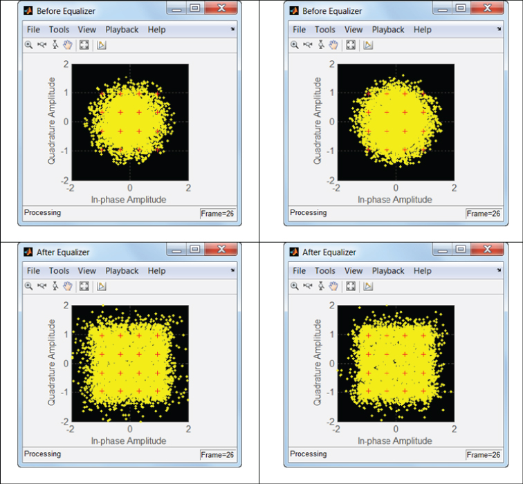
This means that by looking at the constellation of received signals (Figure 8.5) before MIMO detection we can readily see the effects of multipath fading in terms of rotations and attenuations in each of the modulated symbols. If the MIMO and OFDM operations are implemented correctly and do what they are designed to do, the MIMO detector inverts and compensates for the effects of fading channel. A good MIMO detector computes a channel-aware equalizer by first estimating the channel response and then providing the equalization as a counter-measure to all the rotations and attenuations incurred in each symbol. After applying an effective equalizer, the constellation diagram of the recovered symbols following MIMO detection resembles that of the transmitted symbols with additive Gaussian noise around them. As a result, although the channel involves multipath fading following equalization, the effective channel can be approximated by an AWGN channel.
Figure 8.5 Constellation of received signals: before and after MIMO detection
In Chapter 4, we showed that the turbo-coded and modulated symbols transmitted on an AWGN channel are characterized by BER curves that show sharp improvements following a cutoff SNR value. Since after successful MIMO detection the effective channel is an AWGN channel in the LTE system, the system will have the same pattern of BER curve as a function of the SNR.
Figure 8.6 shows BER curves from a system simulation model executed for a range of SNR values. The model operates in transmission mode 4, using a frequency-selective channel with all the parameters of the lower-distortion channel model specified in the last section. Note how they reflect the same structure and pattern, as if the AWGN channel were the only channel model present. This means that the frequency-domain equalization furnished by the MIMO detection effectively compensates for the effects of multipath fading. As we can see in Figure 8.6, the results are quite prominent for the QPSK and 16QAM modulation schemes. In the case of 64QAM modulation, if we use an approximate channel-estimation technique we will have a less prominent drop in the BER curve.
Figure 8.6 BER as a function of an SNR–LTE simulation model with frequency-selective fading channel: QPSK (left), 16QAM (middle), 64QAM (right)

8.3.3 Effects of Channel-Estimation Techniques
In this section we examine BER performance as a function of channel-estimation methods. The experiment provides similar results in different transmission modes. For example, we run the system model in transmission mode 4 with a frequency-selective channel and with all parameters of the lower-distortion channel model previously specified. The experiment is performed by changing one of four channel-estimation techniques, simply by changing the prmMdl.chEst parameter in the commlteSystem_params MATLAB script. The results are summarized in Table 8.3. As expected, the ideal channel estimator provides the best BER performance. The estimation based on interpolation allows for the most variation within slots and subframes and thus has a higher performance in an MMSE error-minimization context. When averaging in time across slots or subframes, we smooth out the spectrum. These averaging methods do not therefore improve the BER performance results but may provide the continuity and smoothness needed for better perceptual results. We will verify this effect in the next section, where we process actual voice data through our simulation model and focus on perceived voice quality.
Table 8.3 Sample of BER results as a function of channel-estimation technique
| Channel-estimation method | BER |
| Ideal estimation | 0.0001 |
| Interpolation-based | 0.0056 |
| Averaging over each slot | 0.0076 |
| Averaging over a subframe | 0.0086 |
8.3.4 Effects of Channel Models
In this section we examine BER performance as a function of different channel models. The experiment provides similar results in different transmission modes. We use transmission mode 2 (transmit diversity) with a 2 × 2 antenna configuration and iterate through multiple channel models. This includes user-defined flat and frequency-selective fading models and all 3GPP LTE channel models. We also sweep through various mobility measures expressed as either 0, 5, or 70 Hz maximum Doppler shifts and iterate through different profiles of antenna spatial correlations. Keeping the link SNR to a constant value of 13 dB and using a 16QAM modulation scheme, the experiment iterates through channel models by changing the chanMdl parameter structure, specifically by changing the maximum Doppler shift (chanMdl.Doppler) and the spatial correlation (chanMdl.corrLvl) parameters in the commlteSystem_params MATLAB script. Table 8.4 summarizes the results.
Table 8.4 BER performance as a function of channel model

As we increase the extent of the noise profile (using EPA, Extended Pedestrian A, and EVA, Extended Vehicular A), the performance becomes consistently reduced. Higher mobility has an adverse effect on the performance. Also, by increasing the spatial correlations, we increase the chance of rank deficiency in the channel matrix, with detrimental effects on quality.
8.3.5 Effects of Channel Delay Spread and Cyclic Prefix
As discussed earlier, the CP length is an important parameter in the OFDM transmission methodology. If path delays in a channel model correspond to values greater than the CP length, the OFDM transmission cannot maintain orthogonality between subcarriers in the receiver. This will have a detrimental effect on the BER quality of the transceiver.
The LTE standard allows the scheduler to provide both normal and extended CP lengths. In propagation environments with high delay spreads, we can switch to transmissions that employ extended CP lengths, which can help improve performance.
As shown in Table 8.5, all transmission bandwidths with normal CP lengths have a constant maximum delay spread of about 4.6875 µs. We verify in this section that when employing user-defined frequency-selective channel models, setting the path delays to different values relative to the CP lengths can have a significant impact on BER performance. We implement this experiment by altering the way in which the path delays of the user-specified frequency-selective channel models are specified. In the following MATLAB code, we determine the path delays as equally-spaced samples between 0 and the maximum delay value.
Table 8.5 Mapping of CP lengths in samples to the channel bandwidth

% Channel parameters
prmMdl.PathDelays = floor(linespace(0,DelaySpread,5))*(1/chanSRate);
In the first case, we use as delay spread a value within the CP length range. The following MATLAB code segment initializes the delay spread as just less than the value of the CP length.
% Channel parameters
chanSRate   = prmLTEPDSCH.chanSRate;
DelaySpread = prmLTEPDSCH.cpLenR - 2;
 prmMdl = prmsMdl(chanSRate,  DelaySpread, chanMdl, Doppler, numTx, numRx, …
    corrLvl, chEstOn, enPMIfback, cbIdx);
In the second case, we use as delay spread a value outside the CP length range. The following MATLAB code segment initializes the delay spread as twice the value of the CP length.
% Channel parameters
chanSRate   = prmLTEPDSCH.chanSRate;
DelaySpread =  2* prmLTEPDSCH.cpLenR;
 prmMdl = prmsMdl(chanSRate,  DelaySpread, chanMdl, Doppler, numTx, numRx, …
    corrLvl, chEstOn, enPMIfback, cbIdx);
The experiment provides similar results in different transmission modes. We have used transmission mode 1 with a 1 × 2 antenna configuration. We applied a constant link SNR value of 15 dB and used a 16QAM modulation scheme. The results are summarized in Table 8.6. We observe that having delay spread values that occasionally exceed the maximum CP length can result in severe performance degradations.
Table 8.6 Effect of delay spread range on BER performance
| Delay spread value | BER |
| Low | 0.00019 |
| High | 0.02440 |
8.3.6 Effects of MIMO Receiver Algorithms
In this section, we examine BER performance as a function of different MIMO receiver algorithms. Simply by changing the equalization mode (represented by the prmLTEPDSCH.Eqmode parameter) to a value of 1, 2, or 3, we can examine a Zero Forcing (ZF), MMSE, and sphere-decoder algorithm, respectively. Table 8.7 summarizes the results.
Table 8.7 Effect of a MIMO detection algorithm on BER performance
| MIMO detection method | BER |
| ZF algorithm | 0.0001 |
| MMSE algorithm | 0.0056 |
| Soft-sphere decoding | 0.0076 |
Although the ZF algorithm provides the simplest implementation, by ignoring the noise power at the receiver, it results in the lowest BER performance. The BER performance of the MMSE algorithm is better than its ZF performance. It is formulated to essentially invert the channel matrix while taking into account the power of the noise. However, the best performance is furnished by the sphere decoder, which uses maximum-likelihood decoding to optimize for the modulation symbols based on their symbol mapping. A sphere decoder is an algorithm of relatively high computational complexity and the time it takes to process a sphere-decoder receiver can be substantially greater than for an MMSE receiver. As such, the choice between a MIMO receiver based on MMSE and on a sphere decoder represents a classical tradeoff between complexity and performance.
8.4 Throughput Analysis
LTE-standard documents provide not only the transmitter specifications but also channel conditions for testing and the minimum performance criteria needed to qualify for standard compliance. For example, the standard document TS 36.101 provides all minimum performance requirements for downlink transmission. An excerpt from this document is illustrated in Figure 8.7. As an example, a single throughput requirement for the SIMO transmission mode is captured as a set of test cases in which various parameters are given as inputs and the expected throughput is given as output. Input specifications include the bandwidth, reference channel, propagation (channel mode), antenna spatial correlation matrix, and reference SNR values. Throughput is defined as the average data rate for which successful transmission occurs. Maximum throughput corresponds to the case where no input block with errors is received. The relative throughput is the fraction of successful transmission with respect to maximum throughput. For example, test case 1, corresponding to QPSK (Quadrature Phase Shift Keying) modulation, expects a 70% relative throughput for an SNR value of −1 dB when the EVA channel model with a Doppler shift of 5 Hz is used with low spatial antenna correlations and a transmission mode of 1 is used with a 1 × 2 antenna configuration and a bandwidth of 10 MHz.
Figure 8.7 Test cases for LTE downlink compliance: TS 36.101 excerpt on minimum requirement testing 2. Courtesy of 3GPP documentation

We have modified our receiver and the system MATLAB functions for computation of the throughput. In the receiver, as the last processing step we compute CRC detection. When any error is found in CRC detection, the block of output is deemed to have been received in error. By excluding all erroneous blocks from the total number of blocks processed we can find the relative throughput as the ratio of correctly received blocks to total received blocks. The following MATLAB function uses this definition to compute and display the relative throughput.
function Throughput=getThroughput( ber, CbFlag, SubFrame)
persistent ErrorBlk
if isempty(ErrorBlk)
    ErrorBlk=0;
end
ErrorBlk = ErrorBlk + CbFlag;
Throughput=1-(ErrorBlk/SubFrame);
fprintf(1,'Subframe %4d ; BER = %6.4f ; ErrorFrame = %4d ; Throughput = %4.2f
', …
        SubFrame, ber, ErrorBlk, Throughput );
end
8.5 System Model in Simulink
So far we have presented MATLAB algorithms and testbenches to simulate the PHY of the LTE standard. In this section we show how expressing the same system model as a Simulink model facilitates our design process. Simulink models naturally provide a simulation testbench, which enables us to focus on algorithms and their updates rather than having to maintain the testbench. Let us take a look at our MATLAB system model in order to distinguish its algorithmic portions (i.e., code related to system processing) from its testbench components (i.e., code related to maintaining a simulation framework).
clear functions
commlteSystem_params;
[prmLTEPDSCH, prmLTEDLSCH, prmMdl] = commlteSystem_initialize(txMode, …
    chanBW, contReg, modType, Eqmode,numTx, numRx,cRate,maxIter, fullDecode,
chanMdl, Doppler, corrLvl, …
    chEstOn, numCodeWords, enPMIfback, cbIdx);
clear txMode chanBW contReg modType Eqmode numTx numRx cRate maxIter
fullDecode chanMdl Doppler corrLvl chEstOn numCodeWords enPMIfback cbIdx
%%
disp('Simulating the LTE Downlink - Modes 1 to 4');
zReport_data_rate_average(prmLTEPDSCH, prmLTEDLSCH);
hPBer = comm.ErrorRate;
%% Simulation loop
tic;
SubFrame =0;
nS = 0; % Slot number, one of [0:2:18]
Measures = zeros(3,1); %initialize BER output
while (Measures(3) < maxNumBits) && (Measures(2) < maxNumErrs)
____________________________________________________________________
    %% Transmitter
    [txSig, csr, dataIn] = commlteSystem_Tx(nS, prmLTEDLSCH, prmLTEPDSCH, prmMdl);
     %% Channel model
     [rxSig, chPathG, ˜]  = commlteSystem_Channel(txSig, snrdB, prmLTEPDSCH,  prmMdl );
     %% Receiver
     nVar=(10.^(0.1.*(-snrdB)))*ones(1,size(rxSig,2));
     [dataOut, dataRx, yRec] = commlteSystem_Rx(nS, csr, rxSig, chPathG, nVar, …
         prmLTEDLSCH, prmLTEPDSCH, prmMdl);
– –  –  –  –  –  –  –  –  –  –  –  –  –  –  –  –  –  –  –  –  –  –  –  –  –  –  –  –  –  –  –  –  –  –  –  –
____________________________________________________________________
    %% Calculate  bit errors
    Measures = step(hPBer, dataIn, dataOut);
    %% Visualize results
    if (visualsOn && prmLTEPDSCH.Eqmode˜=3)
        zVisualize( prmLTEPDSCH, txSig, rxSig, yRec, dataRx, csr, nS);
    end;
    fprintf(1,'Subframe no. %4d ; BER = %g
', SubFrame, Measures(1));
    %% Update subframe number
    nS = nS + 2; if nS> 19, nS = mod(nS, 20); end;
    SubFrame =SubFrame +1;
end
– –  –  –  –  –  –  –  –  –  –  –  –  –  –  –  –  –  –  –  –  –  –  –  –  –  –  –  –  –  –  –  –  –  –  –  –
toc;
We can identify three main portions in the MATLAB system model:
When we express the same model in Simulink, we essentially focus on modeling the in-loop processing. The scheduling is handled by Simulink. With its time-based simulation engine, Simulink iterates through samples or frames of data until the specified simulation time or a stopping condition has been reached. Since MATLAB and Simulink share data in MATLAB workspace, we can either perform the initialization commands manually before simulating the Simulink model or set the Simulink model up to perform the initialization code when the model opens or at any time before the simulation starts.
In the following sections, we go through a step-by-step process of expressing the transceiver in Simulink. First, we create a Simulink model and integrate the MATLAB algorithms developed so far as distinct blocks within it. Then we set the initialization routines up automatically and make parameterizations easier by creating a parameter dialog.
8.5.1 Building a Simulink Model
We can build the Simulink model expressing the LTE transceiver system by using blocks from the Simulink library. The Simulink library can be accessed by clicking on the Simulink Library icon in the MATLAB environment, as illustrated in Figure 8.8. Within the Simulink library browser, various collections of blocks from Simulink and other MathWorks products can be found. We will be using mostly blocks from Simulink, the DSP System Toolbox, and the Communications System Toolbox. As an example, Figure 8.9 illustrates a library of Simulink blocks called the User-Defined Functions.
Figure 8.8 Accessing Simulink library from within the MATLAB environment

Figure 8.9 Simulink block libraries, organized as a main Simulink library and other product libraries

To start building a new Simulink model, we can use the Menu bar of the Simulink library browser and make the following selections: File → New → Model. An empty Simulink model will appear, as shown in Figure 8.10.
Figure 8.10 Building a new Simulink model for an LTE transceiver: start with an empty model

8.5.2 Integrating MATLAB Algorithms in Simulink
Next, we populate this system with blocks step by step in order to represent the LTE transceiver in Simulink using previously developed MATLAB algorithms.
Since we are planning to reuse the MATLAB algorithms developed for the transmitter, channel model, and receiver, we need blocks that can turn a MATLAB function into a component of the Simulink model. The block that can perform this task is called the MATLAB Function block and can be found under the Simulink User-Defined Functions library. We need to add four copies of the MATLAB Function block to our model. As shown in Figure 8.11, we can change the block names to identify their functionalities as follows: Transmitter, Channel, Receiver, and Subframe Update.
Figure 8.11 Adding MATLAB Function blocks to the Simulink model

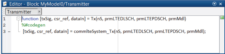
As the next step we open the Transmitter block by double clicking on its icon. As we open any MATLAB Function block, a default function definition will open in the MATLAB Editor, as illustrated in Figure 8.12. Now we can modify the default function definition to implement our function. As we define the function, the input arguments of the function become the input ports of the block and the output arguments of the function become the output ports of the block.
Figure 8.12 The MATLAB Function block, with a default function definition

At this point we have two choices. We can either copy the body of our transmitter function (commlteSystem_Tx) and paste it under the function definition line or we can make a function call to our transmitter function, as illustrated by Figure 8.13, in order to relate the input variables of the function definition to its output variables.
Figure 8.13 MATLAB Function block: updating function definition to implement the transmitter
After saving this function, we can go back to the parent model by clicking on the Go to Diagram icon. As shown in Figure 8.14, we will see that the Transmitter block is transformed to reflect the new function definition. At this stage, by default all function arguments are mapped to corresponding input and output ports.
Figure 8.14 Simulink model with an updated Transmitter block definition without any parameters

We would like to turn all the relevant parameter structures (prmLTEDLSCH, prmLTEPDSCH, prmMdl) into parameters of the Simulink model. These parameter structures will have constant values during the simulation and will be accessed by the Simulink model as three variables in the MATLAB workspace. We open the Transmitter block and in the MATLAB Editor click on the Edit Data icon above the Editor, as illustrated in Figure 8.15.
Figure 8.15 Accessing the Ports and Data Manager to express transmitter LTE structure arguments as model parameters

A dialog called Ports and Data Manager appears, which enables us to edit data properties and manage ports and parameters. This dialog is shown in Figure 8.16. Next, we click on each of the port names (prmLTEDLSCH, prmLTEPDSCH, prmMdl), change the Scope property into a Parameter, uncheck the Tunable checkbox to mark the parameter as a constant, and click on the Apply button.
Figure 8.16 Setting LTE parameter structures as nontunable parameters

We then repeat these operations for the Channel and the Receiver MATLAB Function blocks. Figure 8.17 illustrates simple MATLAB function calls made inside the Channel and the Receiver MATLAB Function blocks, which allow us to directly integrate algorithms developed previously in MATLAB as blocks in Simulink.
Figure 8.17 Calling Channel Model and Receiver functions inside corresponding MATLAB Function blocks

At this stage we can connect the output signal of the Transmitter block (txSig) to the input port of the Channel block. We also connect the three output signals of the Channel block (rxSig, chPathG, nVar) to the input ports of the Receiver block, as illustrated in Figure 8.18.
Figure 8.18 Connecting Transmitter, Channel Model, and Receiver blocks

Now we have to update the subframe number (nS). The subframe number is the common input to both the Transmitter and the Receiver blocks. To avoid excessive wiring in the model, we use the GoTo and the From blocks from the Simulink Signal Routing library. The output of the Subframe Update MATLAB Function block is the slot number of the current frame. We connect this output signal to a GoTo block and, after clicking on the block, assign this signal an identifier, otherwise known as the tag of the block. Now, any From block in the model bearing the same tag can route the signal to multiple blocks in the model. As illustrated in Figure 8.19, we have used two From blocks to connect the subframe number to both the Transmitter and the Receiver blocks.
Figure 8.19 Using GoTo and From blocks to connect the subframe number to both the transmitter and the receiver

When we double click the Subframe Update MATLAB Function block we find the MATLAB function illustrated in Figure 8.20. This is the same code used previously in our MATLAB testbenches to update the subframe number. We have used a persistent variable here to implement the subframe update operation as a counter that resets its value in every 10 ms frame. Now we use additional GoTo and From blocks to finalize block connectivity in the model. As illustrated in Figure 8.21, the pair of GoTo and the From blocks is identified by a selected tag (csr) and a purple background color. This ensures that the same cell-specific reference signal (pilot) computed in the transmitter is also used in the receiver in the same subframe. We also use two other GoTo blocks to collect the transmitted input bit stream (dataIn) and the receiver output bit stream (dataOut). We use the tags Input and Output for the signals dataIn and dataOut, respectively, in the GoTo blocks, and use the same background color. To compute the BER of the system, we use the Error Rate Calculation block from the CommSinks Simulink library of the Communications System Toolbox. Using two From blocks with the tags Input and Output, we route the transmitted input stream and receiver output stream to the Error Rate Calculation block, as illustrated in Figure 8.22. The Error Rate Calculation block compares the decoded bits with the original source bits per subframe and dynamically updates the BER measure throughout the simulation. The output of this block is a three-element vector containing the BER, the number of error bits observed, and the number of bits processed.
Figure 8.20 Subframe Update MATLAB function block implemented as a counter

Figure 8.21 Improved block port connectivities using GoTo and From block pairs

Figure 8.22 Completing the in-loop processing specification in Simulink with BER calculation

The model checks the Stop Simulation parameter of the Error Rate Calculation block in order to control the duration of the simulation (Figure 8.23). The simulation stops upon detection of the target value for whichever of the following two parameters comes first: the maximum number of errors (specified by the maxNumErrs parameter) or the maximum number of bits (specified by the maxNumBits parameter).
Figure 8.23 The Error Rate Calculation block controlling the duration of the simulation

At this point we have completed the in-loop processing specification in our Simulink model. The next steps include initializing the model with LTE parameter structures and running the Simulink model. Simulink model parameters can be initialized in multiple ways, but we will look at two here: (i) setting model properties as the model is opened and (ii) using a mask subsystem to provide a parameter dialog.
8.5.3 Parameter Initialization
Some operations in a system model get executed only once before the simulation loop starts. Such operations represent system initialization. All the operations specified so far in our Simulink model are part of the processing loop and are repeated in simulation iterations. One way of specifying initialization operations in Simulink is to use the Model Properties and in particular the Callback functions.
As illustrated in Figure 8.24, we can access the Model Properties by using the Menu bar of our model and making the following selections: ![]()
Figure 8.24 Accessing the Model Properties of a Simulink model

As we open the Model Properties dialog, we find multiple Model Callbacks under the Callbacks tab. Associated with each type of Model Callback, we find an edit box where MATLAB functions or commands can be executed. The type of callback relates to each stage of simulation. For example, in Figure 8.25 we have selected the PreLoadFcn callback. This means initialization functions, identical to the ones executed before the while loop in our MATLAB model, will execute as we load (or open) the Simulink model.
Figure 8.25 Specifying initialization commands as the PreLoadFcn callback

At this point, the Simulink model is specified both for initialization operations and for in-loop processing. Initialization routines are performed when we open the model and the simulation starts when we click on the Run button. The final step is to specify the Simulink solver and, if need be, set the sample time for the simulation. We can access Simulink solvers by using the Menu bar of our model and making the following selections: ![]() Since we are performing a digital baseband simulation of a communications system, the simulation uses discrete-time sampling. Therefore, as illustrated in Figure 8.26, under the Solver Options properties, we should use Fixed-Step as the Type and Discrete (No Continuous State) as the Solver. These options are typical for most Simulink models simulating DSP or Communications System Models with no analog or mixed-signal components.
Since we are performing a digital baseband simulation of a communications system, the simulation uses discrete-time sampling. Therefore, as illustrated in Figure 8.26, under the Solver Options properties, we should use Fixed-Step as the Type and Discrete (No Continuous State) as the Solver. These options are typical for most Simulink models simulating DSP or Communications System Models with no analog or mixed-signal components.
Figure 8.26 Setting Solver Options, Sample Time, and Stop Time for the simulation model

In addition, since we stop the simulation based on parameters of the Error Rate Calculation block, we specify any value as the Stop Time in this dialog. Here we select a maximum value of infinity (specified by the inf parameter). Furthermore, since the unit of processing is a subframe with a duration of 1 ms, in the edit box for the property Fixed-Step Size (Fundamental Sample Time) we set a value of 0.001 seconds.
Now the specification phase of our Simulink model is complete and we can run the model to test whether (i) the initialization routines performed as CallBacks are implemented correctly and (ii) the transceiver works as intended.
We save the model and then close it. After opening the model again, all three LTE parameter structures (prmLTEDLSCH, prmLTEPDSCH, prmMdl) and three additional parameters (snrdB, maxNumBits, maxNumErrs) are automatically generated in the MATLAB workspace. This verifies the proper operations of our CallBack routines, as illustrated in Figure 8.27.
Figure 8.27 Opening the model and automatically generating simulation parameters using CallBacks

8.5.4 Running the Simulation
Through simulation, we can test the proper operation of the transceiver. We execute the simulation by clicking the Run button on the Model Editor displaying the model. Running the simulation causes the Simulink engine to convert the model to an executable form, in a process known as model compilation. As its first compilation step, the Simulink engine checks for consistency in the model by evaluating the model's block parameter expressions, determining attributes of all signals and verifying that each block can accept the signals connected to its inputs.
Since our model is composed of MATLAB Function blocks, at this stage the Simulink engine first converts the MATLAB code inside the MATLAB Function blocks to C code and then compiles the generated C code to create an executable for each MATLAB Function block of the model. If any MATLAB Function blocks contain MATLAB codes that are not supported by code generation, we have to modify them. Finally, in the linking phase data memory is allocated for each signal and all compiled executable are linked together and made ready for execution.
Simulation errors may occur, either at the model compilation time or at run time. In case of simulation errors, Simulink halts the simulation, opens the component that caused the error, and displays pertinent information regarding the error in the Simulation Diagnostics Viewer. An example is illustrated in Figure 8.28, which shows how the Simulink engine accurately checks the consistency of the port connection between blocks in the model; the Simulink engine has inferred that the subframe number (nS) signal affects the sizes of transmitted and received bit (dataIn and dataOut) signals. So in each subframe, the size of these two signals may change. However, by default, if we do not specify the sizes of any signal in any MATLAB Function block, the signal is assumed to be of a constant size. This “variable-size” nature of the two signals is the subject of the error message shown in Figure 8.28.
Figure 8.28 Simulation error displayed by Simulink regarding the size of the transmitted signal

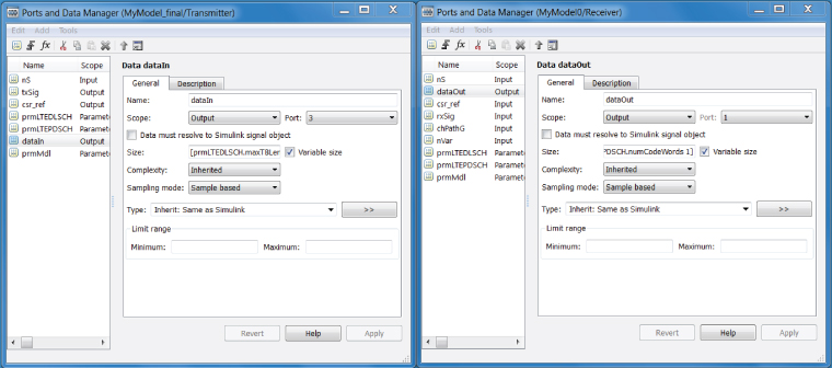
To fix this compilation problem, we need to mark both the dataIn and dataOut signals as variable-size signals and specify their maximum size. We need to double click on both the Transmitter and Receiver blocks, access their Port and Data Manager dialogs, as described before, select the dataIn and dataOut output signals, and change their Size properties by clicking on the Variable Size checkbox and specifying the maximum size. These steps are illustrated in Figure 8.29.
Figure 8.29 Configuring Transmitter and Receiver output signals as variable size and setting their maximum size
This type of variable-size signal handling is typical in Simulink models that express communications systems. This is in part due to the fact that during a simulation the sizes of various signals can change from one frame to another.
Now we can successfully run the simulation by clicking on the Run button. The simulation will proceed until a specified number of bits are processed. The simulation stops as the Error Rate Calculation block detects the stopping criteria. The BER results are shown in Figure 8.30.
Figure 8.30 Running the Simulink system model and measuring BER performance

The performance results reflect the system parameters specified during initialization in the MATLAB script (commlteSystem_params). If we want to run the simulation for a different transmission mode or a different set of operating conditions, we must first modify the system parameters by changing the MATLAB script. Then we need to return to our Simulink model and rerun the simulation. This process of iterating between MATLAB and Simulink for parameter specification can become tedious if we run multiple simulations. To make parameter specification easier, in the next section we develop a parameter dialog in Simulink.
8.5.5 Introducing a Parameter Dialog
Parameter dialogs facilitate updates to the system parameters and enhance the way in which we specify simulation parameters directly and graphically in Simulink. Essentially, we need to introduce a new subsystem in our Simulink model that contains all the model parameters and allows us to easily update them. This special kind of subsystem is known as a masked subsystem.
A subsystem is a collection of one or more blocks in a Simulink model. Every subsystem can be masked; that is, it can have a dialog in which the subsystem parameters are specified. However, in this section we introduce a subsystem whose purpose is to contain and update the model parameters. As illustrated in Figure 8.31, we start by adding a Subsystem block from the Ports and Subsystems Simulink library into our model.
Figure 8.31 Introducing a subsystem to a Simulink model from the Ports and Subsystems Simulink library

As we double click the Subsystem block icon to open it, we notice that it contains a trivial connection from an input port to an output port. Note that in this section, we are not actually building a subsystem but rather using the Subsystem block to create a masked subsystem in order to hold our system parameters. As a result, our first action is to remove the input and output ports and the connector from the Subsystem block. The subsystem will now be empty, as illustrated in Figure 8.32. To distinguish this Subsystem from the other blocks and subsystems of our model, we change its background color and rename it Model Parameters, as shown in Figure 8.33.
Figure 8.32 Making an empty subsystem to focus on masking and introducing parameters
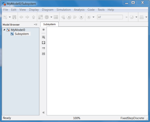
Figure 8.33 Changing our subsystem background color and changing its name to Model Parameters

The next step is to turn our empty subsystem into a masked subsystem. As illustrated by Figure 8.34, this is easily done by first clicking on the subsystem to select it and then using the Menu bar of the model to make the following selections: ![]() When we turn a subsystem into a masked subsystem, double clicking on the Subsystem icon no longer opens the subsystem to display its content. Rather, a mask editor opens, enabling us to add and specify various parameters and to initialize them. Figure 8.35 shows an empty mask editor for our Model Parameters subsystem.
When we turn a subsystem into a masked subsystem, double clicking on the Subsystem icon no longer opens the subsystem to display its content. Rather, a mask editor opens, enabling us to add and specify various parameters and to initialize them. Figure 8.35 shows an empty mask editor for our Model Parameters subsystem.
Figure 8.34 Turning the Model Parameters subsystem into a masked subsystem

Figure 8.35 Opening the Model Parameters mask editor in order to introduce parameters

A mask editor contains four tabs: the Icon and Ports tab allows us to display text and images on the subsystem icon, the Parameters tab allows us to introduce parameters and specify what values they can take, the Initialization tab allows us to include MATLAB functions that operate on the subsystem parameters and help us create various system parameters in the MATLAB workspace, and the Documentation tab allows us to display text containing information about the subsystem when we double click on the subsystem to open the dialog.
In this section, we customize the mask editor within the Parameters and Initialization tabs. Fist, we introduce our operating parameters one by one under the Dialog Parameters list of the Parameters tab, as illustrated in Figure 8.36. To add a new parameter to the list, we click on the first icon in the upper left-hand side of the Dialog Parameters list, called Add Parameters. A new list item will be added to the Dialog Parameters list, containing fields such as Prompt, Variable, Type, and so on. In the Prompt field, we specify the text that will appear in the dialog next to the parameter. In the Variable field, we specify the name of the MATLAB variable to be used in the initialization stage later. The Type field specifies the way we assign values to the parameter. If we choose an edit box, we specify the actual value of the parameter in an edit box in the dialog. If we choose a check box, the parameter is specified as a Boolean choice with a value of true if the condition expressed in the Prompt field holds and a value of false otherwise.
Figure 8.36 Adding parameters one by one to the Dialog Parameters list in the Parameters tab

If we choose a popup, we specify the parameter as a choice among a finite number of choices. These choices are enumerated in the Type-Specific Options list in the lower left-hand corner of the Parameters tab. For example, for the transmission mode (txMode) parameter, as illustrated in Figure 8.36, we choose a popup and then list all four choices for the transmission mode (SIMO, TD, open-loop SM, closed-loop SM) in the Type-Specific Options list associated with the txMode parameter.
At this point we can see how the parameter dialog looks after specifying the first parameter. To do so we save and close the mask editor, go back to the model, and double click on the Model Parameters subsystem icon. As illustrated in Figure 8.37, a Block Parameters dialog will appear, bearing the name of the subsystem. So far, only one icon (Transmission Mode) has appeared under the Parameters list, matching exactly what we typed in the parameter prompt field. Note that in front of the prompt, we find a popup menu with the four choices for the transmission mode, matching exactly what we typed in the Type-Specific Options list associated with the parameter.
Figure 8.37 Inspecting the parameter dialog and how it reflects parameter lists developed under the mask editor

We can now repeat the process of adding parameters to the parameter list in the mask editor. Note that we need to add as many parameters as there are in the MATLAB script (commlteSystem_params) in order to generate all three LTE parameter structures (prmLTEDLSCH, prmLTEPDSCH, prmMdl) and all three additional parameters (snrdB, maxNumBits, maxNumErrs) for our system simulation in Simulink. One particular instance of the MATLAB parameter script (commlteSystem_params) is shown as a reference:
%% Set simulation parametrs & initialize parameter structures
txMode             = 4;   % Transmisson mode one of {1, 2, 3, 4}
numTx              = 2;    % Number of transmit antennas
numRx              = 2;    % Number of receive antennas
chanBW            = 4;    % [1,2,3,4,5,6] maps to [1.4, 3, 5, 10, 15, 20]MHz
contReg            = 2;     % {1,2,3} for >=10MHz, {2,3,4} for <10Mhz
modType           = 2;     % [1,2,3] maps to ['QPSK','16QAM','64QAM']
numCodeWords  = 1;   % Number of codewords in PDSCH
% DLSCH
cRate                = 1/2;  % Rate matching target coding rate
maxIter              = 6;     % Maximum number of turbo decoding terations
fullDecode         = 0;     % Whether "full" or "early stopping" turbo decoding is performed
% Channel
chanMdl          = 'EPA 0Hz';  % one of {'flat','frequency-selective', 'EPA 0Hz', 'EPA 5Hz', 'EVA 5Hz', 'EVA 70Hz'}
Doppler            = 0;                                 % a value between 0 to 300 = Maximum Doppler shift
corrLvl              = 'Low';                          %  one of {'Low', 'Medium', 'High'} Spatial correlation level between antennas
enPMIfback    = 0;     % Enable/Disable Precoder Matrix Indicator (PMI) feedback
cbIdx               = 1;      % Initialize PMI index
% Simulation parametrs
Eqmode           = 2;      % Type of equalizer used [1,2,3] for ['ZF', 'MMSE','Sphere Decoder']
chEstOn           = 1;          % use channel estimation or ideal channel
snrdB = 12.1;
maxNumErrs     = 2e6; % Maximum number of errors found before simulation stops
maxNumBits     = 2e6;  % Maximum number of bits processed before simulation stops
Figure 8.38 shows how we can add and populate parameters in the mask editor to bear the same variable names as found in the MATLAB parameter script commlteSystem_param.
Figure 8.38 Adding to the parameter list and matching variable names to ones specified in the MATLAB script

After saving and closing the mask editor, we can inspect the parameter dialog once we have specified all the parameters. As illustrated in Figure 8.39, specifying parameters using a masked subsystem in Simulink is the most convenient approach. We no longer need to edit and save the MATLAB parameter script in the MATLAB editor, come back to the Simulink model, and rerun the simulation. All parameters can now be specified in the Simulink model using an intuitive parameter dialog.
Figure 8.39 A convenient parameter dialog for setting LTE system model parameters in the Simulink model

It is beneficial to the process of parameter initialization, as we will see shortly, to match variable names in the mask editor to those in the MATLAB parameter script. All that is needed now is to run the initialization commands in the Initialization tab of the mask editor that generates the LTE parameter structures based on the parameter dialog values. As illustrated in Figure 8.40, the parameter dialog variables are listed in the left-hand side of the Initialization tab. On the right-hand side we find an Initialization Commands edit box. In this edit box we can type various MATLAB commands or call a MATLAB function. Here, we are calling a MATLAB function (commlteMIMO_Simulink_init) to generate model parameters from the dialog variables and put them in the MATLAB workspace.
Figure 8.40 Initialization commands in the mask editor generating LTE parameter structures from the parameter dialog

Since the variable names we chose in the mask editor are identical to those in the MATLAB parameter script, the masked subsystem initialization function commlteMIMO_Simulink_init is almost identical to the MATLAB initialization function we used in our MATLAB system model (commlteSystem_initialize).
function commlteMIMO_Simulink_init(txMode, Tx, Rx, chanBW,  modType, contReg,…
     numCodeWords, cRate,maxIter, fullDecode, …
    chanMdl, snrdB, Doppler, corrLvl, maxNumBits, cbIdx,  Eqmode, chEstOn )
% Create the parameter structures
vector=[1,2,4];
numTx=vector(Tx);
numRx=vector(Rx);
% PDSCH parameters
CheckAntennaConfig(numTx, numRx, txMode, numCodeWords);
prmLTEPDSCH = prmsPDSCH(txMode, chanBW, contReg, modType, numTx, numRx, numCodeWords,Eqmode);
[SymbolMap, Constellation]=ModulatorDetail(prmLTEPDSCH.modType);
prmLTEPDSCH.SymbolMap=SymbolMap;
prmLTEPDSCH.Constellation=Constellation;
if numTx==1
    prmLTEPDSCH.csrSize=[2*prmLTEPDSCH.Nrb, 4];
else
    prmLTEPDSCH.csrSize=[2*prmLTEPDSCH.Nrb, 4, numTx];
end
% DLSCH parameters
prmLTEDLSCH = prmsDLSCH(cRate,maxIter, fullDecode, prmLTEPDSCH);
% Channel parameters
chanSRate   = prmLTEPDSCH.chanSRate;
DelaySpread = prmLTEPDSCH.cpLenR;
 prmMdl = prmsMdl( chanSRate,  DelaySpread, chanMdl, Doppler, numTx, numRx, …
    corrLvl, chEstOn-1, 0, cbIdx);
%% Assign parameter structure variables to base workspace
assignin('base', 'prmLTEPDSCH', prmLTEPDSCH);
assignin('base', 'prmLTEDLSCH', prmLTEDLSCH);
assignin('base', 'prmMdl', prmMdl);
assignin('base', 'snrdB', snrdB);
assignin('base', 'maxNumBits', maxNumBits);
assignin('base', 'maxNumErrs', maxNumBits);
Note that the main difference between this initialization function and the one used in our MATLAB model is the addition of six lines at the end of the function. These extra lines take the variables defined locally in the scope of the function and write them to the MATLAB workspace.
8.6 Qualitative Assessment
As the last topic in this chapter, we perform a qualitative assessment of our LTE system model. Instead of processing randomly generated payload bits, we can process the bit stream of a voice signal. In a sense, this experiment simulates a phone conversation over the simulated LTE PHY model.
8.6.1 Voice-Signal Transmission
The first step of qualitative assessment is to introduce speech coding. In this step, we encode the voice signal and pass the encoded bit stream as input to the LTE transceiver model. We are using one of the simplest voice-coding algorithms, based on either A-law or μ-law Pulse Code Modulation (PCM) coding. At the receiver, we apply the corresponding A-law or μ-law decoder to the recovered bit stream of the LTE model in order to obtain the output voice signal and listen to the speech. The quality of the recovered voice signal reflects all the degradations introduced by the channel and the receiver.
To simulate the LTE phone call, we use the Simulink model we developed in the last section. The only modifications needed (Figure 8.41) are related to the encoding and decoding of the voice signal:
Figure 8.41 Modified Simulink model combining speech encoding and decoding with an LTE transceiver model to measure voice quality

The speech coding sequence is implemented as follows:
The speech decoding sequence inverts the speech coding operations as follows:
8.6.2 Subjective Voice-Quality Testing
We can simulate the model for various conditions, including the SIMO, transmit-diversity, and spatial-multiplexing transmission modes. As we listen to the speech file output, we note that the quality of the voice signal depends on the parameters of the transceiver and the channel model. For example, if the fading delay spread, as reflected in the fading-channel path-delay parameter, is within 4.6 µs (as prescribed by the standard) then the SNR in recovering speech will be within representative values and the perceived speech quality will be reasonably good. Similarly, by using modes with improved link quality, such as transmit diversity instead of SISO (Single Input Single Output), we can obtain a better voice quality.
8.7 Chapter Summary
In this chapter, we composed a system model for the LTE PHY model. We integrated the first four modes of downlink transmission into the system model comprising the transmitter, the channel model, and the receiver. Then we simulated the system model in order to quantitatively assess the performance of the overall system. We studied the effects of various transmission modes, channel models, link SNRs, channel estimation techniques, MIMO receiver algorithms, and channel delay spreads on the overall performance. We also performed experiments aimed at gauging the throughput of the LTE system model.
Next, we composed a Simulink model for the LTE transceiver model. We built the Simulink model step by step by integrating the MATLAB functions for the transmitter, receiver, and channel model incrementally within the system. We then automated the way we specify the LTE system model parameters by developing parameter dialogs into our Simulink model. Finally, we added a speech coder and decoder to the Simulink model in order to enable a qualitative assessment of the system performance.
References
[1] Jafarkhani, H. (2005) Space-time Coding; Theory and Practice, Cambridge University Press, New York.
[2] 3GPP Evolved Universal Terrestrial Radio Access (E-UTRA); User Equipment (UE) Radio Transmission and Reception (Version 11.4.0), March 2013. TS 36.101.