
Chapter 4
Modulation and Coding
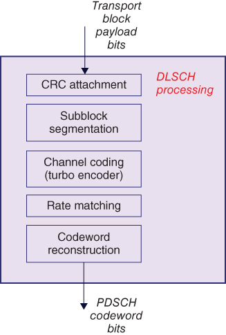
The LTE (Long Term Evolution) downlink PHY (Physical Layer) chain can be viewed as the combination of processing applied to the Downlink Shared Channel (DLSCH) and Physical Downlink Shared Channel (PDSCH). DLSCH processing is also known as Downlink Transport Channel (TrCH) processing. It includes steps involving Cyclic Redundancy Check (CRC) code attachment, data subblock processing, channel coding based on turbo coders, rate matching, Hybrid Automatic Repeat Request (HARQ) processing, and the reconstruction of codewords. The codewords are inputs for the PDSCH processing, which involves scrambling, modulation, multi-antenna Multiple Input Multiple Output (MIMO) processing, time–frequency resource mapping, and Orthogonal Frequency Division Multiplexing (OFDM) transmission. We have subdivided the components of this two-step DLSCH and PDSCH processing chain into three segments, which are discussed in the next three chapters.
In this chapter, we examine the modulation and coding schemes used in the LTE standard. These include all the combined DLSCH and PDSCH processing steps, excluding the MIMO and OFDM operations. Discussion regarding OFDM and MIMO is presented in the next two chapters. First, we will examine the first couple of operations performed in PDSCH processing, including scrambling and modulation. Then we will examine TrCH processing, comprising a series of operations that map logical channels and user bit payload to codewords, which are passed to the shared physical channel.
We will create MATLAB® programs that completely specify the TrCH processing in the transmitter and the receiver. We will use the MATLAB functions to study the effects of different modulation schemes and different coding rates on the Bit Error Rate (BER) performance with an Additive White Gaussian Noise (AWGN) channel model. These operations completely specify how user data bits are processed to produce the input symbols for the subsequent MIMO and OFDM functional blocks for transmission. Details of MIMO and OFDM are then examined in the next two chapters.
4.1 Modulation Schemes of LTE
The modulation schemes used in the LTE standard include QPSK (Quadrature Phase Shift Keying), 16QAM (Quadrature Amplitude Modulation), and 64QAM. Figure 4.1 shows the constellation diagrams of these three modulation schemes.
Figure 4.1 Constellation diagrams of QPSK, 16QAM, and 64QAM

In the case of QPSK modulation, each modulation symbol can have one of four different values, which are mapped to four different positions in the constellation diagram. QPSK needs 2 bits to encode each of its four different modulation symbols. The 16QAM modulation involves using 16 different signaling choices and thus utilizes 4 bits of information to encode each modulation symbol. The 64QAM modulation involves 64 different possible signaling values and thus requires 6 bits to represent a single modulation symbol.
The availability of multiple modulation schemes is instrumental in implementing adaptive modulation based on channel conditions. When the radio link is relatively clean – that is, the Signal-to-Noise Ratio (SNR) is relatively high – we can use modulation schemes of denser constellations, such as 64QAM. In such a case, sending a single symbol results in the transmission of 6 bits and therefore can increase our throughput. However, as the channel becomes noisier, we should resort to using modulation schemes with more intersymbol separation, such as QPSK. This in turn will reduce the number of bits per sample and reduce the throughput.
The LTE modulation mappers, which specify how the modulation symbols are assigned to each bit sequence, are shown in Table 4.1 for QPSK and in Table 4.2 for 16QAM. Due to its large size, we refer the reader to Reference 1 for the standard document on 64QAM modulation mapping.
Table 4.1 Mapping for an LTE QPSK modulator
| Payload bit pattern (2 bits) | Modulated symbol | |
| In-phase (I) | Quadrature (Q) | |
| 00 | ||
| 01 | ||
| 10 | ||
| 11 | ||
Table 4.2 Mapping for an LTE 16QAM modulator
| Payload bit pattern (4 bits) | Modulated symbol | |
| In-phase (I) | Quadrature (Q) | |
| 0000 | ||
| 0001 | ||
| 0010 | ||
| 0011 | ||
| 0100 | ||
| 0101 | ||
| 0110 | ||
| 0111 | ||
| 1000 | ||
| 1001 | ||
| 1010 | ||
| 1011 | ||
| 1100 | ||
| 1101 | ||
| 1110 | ||
| 1111 | ||
We note that the mapping of bits to symbols is based on neither a typical binary nor a gray-coded method. Rather, the LTE specification defines a custom constellation mapping. LTE also defines modulation symbols in such a way that the average signal power is normalized to unity.
4.1.1 MATLAB Examples
As the first step in modeling the LTE downlink processing chain, we start with the LTE modulation schemes. The following two MATLAB functions show how you can easily implement the LTE modulation and demodulation algorithms, with all their specifications, using System objects of the Communications System Toolbox.
function y=Modulator(u, Mode)
%% Initialization
persistent QPSK QAM16 QAM64
if isempty(QPSK)
    QPSK          = comm.PSKModulator(4, 'BitInput', true, …
                          'PhaseOffset', pi/4, 'SymbolMapping', 'Custom', …
                           'CustomSymbolMapping', [0 2 3 1]);
    QAM16      = comm.RectangularQAMModulator(16, 'BitInput',true,…
                           'NormalizationMethod','Average power',
                            'SymbolMapping', 'Custom', …
                            'CustomSymbolMapping',
                            [11 10 14 15 9 8 12 13 1 0 4 5 3 2 6 7]);
    QAM64      = comm.RectangularQAMModulator(64, 'BitInput',true,…
                           'NormalizationMethod','Average power',
                           'SymbolMapping', 'Custom',
                            'CustomSymbolMapping',
                            [47 46 42 43 59 58 62 63 45 44 40 41 …
                            57 56 60 61 37 36 32 33 49 48 52 53 39
                            38  34 35 51 50 54 55 7 6 2 3 19 18 22 23 5
                            4 0 1 17 16 20 21 13 12 8 9 25 24 28 29 15
                            14 10 11 27 26 30 31]);
end
%% Processing
switch Mode
    case 1
        y=step(QPSK, u);
    case 2
        y=step(QAM16, u);
    case 3
        y=step(QAM64, u);
end
The Modulator function has two input arguments: the input bit stream (u) and a parameter representing the modulation mode (Mode). As its output, the function computes the modulated symbols. The function implements the three different types of modulator used in the LTE standard. For example, in the case of QPSK, we use a comm.PSKModulator System object and set its modulation order to 4. Similarly, in the case of 16QAM and 64QAM we use the comm.RectangulatQAMModulator System objects and set their modulation orders to 16 and 64, respectively. Depending on the value of the modulation mode, we process the input bits to generate the modulated symbols as the output.
To ensure that the System object exactly matches what the LTE standard specifies, we can set other properties:
Note that the LTE, like other mobile standards, does not make any recommendations concerning the operations performed in the receiver. Hence, all the receiver specifications presented in this book can be considered typical “inverse” operations of operations specified in the transmitter. These proposed inverse operations represent best efforts to recover the estimate of the transmitted bits. Although not specified in the standard, it is necessary to include these receiver-side inverse operations in order to evaluate the accuracy and performance of the system.
As demodulation is the inverse operation for modulation, we now present some typical approaches to demodulation. In the Demodulator function, we use the same three modulation types used in LTE, and depending on the modulation mode, we process the input symbols to generate the demodulated output. As discussed in the previous section, demodulation can be based on either hard-decision decoding or soft-decision decoding. In hard-decision decoding, the input symbols of a demodulator are mapped to estimated bits, whereas in soft-decision decoding the output is a vector of log-likelihood ratios (LLRs).
The function DemodulatorHard.m shows a demodulation implementation that employs hard-decision decoding. The function takes as inputs the received modulated symbols (u) and the modulation mode (Mode). The function output comprises the demodulated bits.
function y=DemodulatorHard(u, Mode)
%% Initialization
persistent QPSK QAM16 QAM64
if isempty(QPSK)
    QPSK = comm.PSKDemodulator(…
        'ModulationOrder', 4, …
        'BitOutput', true, …
        'PhaseOffset', pi/4, 'SymbolMapping', 'Custom', …
        'CustomSymbolMapping', [0 2 3 1]);
    QAM16 = comm.RectangularQAMDemodulator(…
        'ModulationOrder', 16,  …
        'BitOutput', true, …
        'NormalizationMethod', 'Average power', 'SymbolMapping', 'Custom', …
        'CustomSymbolMapping', [11 10 14 15 9 8 12 13 1 0 4 5 3 2 6 7]);
    QAM64 = comm.RectangularQAMDemodulator(…
    'ModulationOrder', 64, …
    'BitOutput', true, …
    'NormalizationMethod', 'Average power', 'SymbolMapping', 'Custom', …
    'CustomSymbolMapping', …
    [47 46 42 43 59 58 62 63 45 44 40 41 57 56 60 61 37 …
    36 32 33 49 48 52 53 39 38 34 35 51 50 54 55 7 6 2 3 …
    19 18 22 23 5 4 0 1 17 16 20 21 13 12 8 9 25 24 28 29 …
    15 14 10 11 27 26 30 31]);
end
%% Processing
switch Mode
    case 1
        y=QPSK.step(u);
    case 2
        y=QAM16.step(u);
    case 3
        y=QAM64.step(u);
    otherwise
        error('Invalid Modulation Mode. Use {1,2, or 3}');
end
The function DemodulatorSoft.m employs soft-decision decoding to perform demodulation. The function has three input arguments: the received modulated symbol stream (u), the estimate of the noise variance in the current subframe (NoiseVar), and a parameter representing the modulation mode (Mode). As its output, the function computes the LLRs. Examining the differences between the functions, we can see that by setting a couple of properties in the demodulator System objects, including the property called the DecisionMethod, we can implement soft-decision demodulation.
function y=DemodulatorSoft(u, Mode, NoiseVar)
%% Initialization
persistent QPSK QAM16 QAM64
if isempty(QPSK)
    QPSK = comm.PSKDemodulator(…
        'ModulationOrder', 4, …
        'BitOutput', true, …
        'PhaseOffset', pi/4, 'SymbolMapping', 'Custom', …
        'CustomSymbolMapping', [0 2 3 1],…
        'DecisionMethod', 'Approximate log-likelihood ratio', …
        'VarianceSource', 'Input port');
    QAM16 = comm.RectangularQAMDemodulator(…
        'ModulationOrder', 16,  …
        'BitOutput', true, …
        'NormalizationMethod', 'Average power', 'SymbolMapping', 'Custom', …
        'CustomSymbolMapping', [11 10 14 15 9 8 12 13 1 0 4 5 3 2 6 7],…
        'DecisionMethod',  'Approximate log-likelihood ratio', …
        'VarianceSource', 'Input port');
    QAM64 = comm.RectangularQAMDemodulator(…
    'ModulationOrder', 64, …
    'BitOutput', true, …
    'NormalizationMethod', 'Average power', 'SymbolMapping', 'Custom', …
    'CustomSymbolMapping', …
    [47 46 42 43 59 58 62 63 45 44 40 41 57 56 60 61 37 36 32 33 …
    49 48 52 53 39 38 34 35 51 50 54 55 7 6 2 3 19 18 22 23 5 4 0 1 …
    17 16 20 21 13 12 8 9 25 24 28 29 15 14 10 11 27 26 30 31],…
    'DecisionMethod',  'Approximate log-likelihood ratio', …
     'VarianceSource', 'Input port');
end
%% Processing
switch Mode
    case 1
        y=step(QPSK, u, NoiseVar);
    case 2
        y=step(QAM16,u, NoiseVar);
    case 3
        y=step(QAM64, u, NoiseVar);
    otherwise
        error('Invalid Modulation Mode. Use {1,2, or 3}');
end
4.1.2 BER Measurements
The motivation for using multiple modulation methods in LTE is to provide higher data rates within a given transmission bandwidth. The bandwidth utilization is expressed in bits/s/Hz. Compared to the QPSK, the bandwidth utilization of 16QAM and 64QAM is two and three times higher, respectively. However, higher-order modulation schemes are subject to reduced robustness to channel noise. Compared to the QPSK, modulation schemes such as 16QAM or 64QAM require a higher value for Eb/N0 at the receiver for a given bit error probability.
The following MATLAB functions illustrate the first in a series of functions that will eventually implement a realistic transceiver for the LTE PHY modeling in MATLAB. We start with this simple system, which is composed of a modulator, a demodulator, and an AWGN channel, and which computes the BER as a function of the Eb/N0 ratio. By running this function with a series of Eb/N0 values and changing the ModulationMode parameter, we can visualize the relationship between modulation order and robustness to channel noise.
The first function, chap4_ex01.m, uses a demodulator based on hard-decision demodulation, while the second function, chap4_ex02.m, is based on soft-decision decoding. The elements that are common in these two functions, which represent patterns of the series of functions to come, are as follows:
- Signature and input–output arguments
- Size of user payload (input to the PHY) (specified with a parameter (FRM) denoting the number of input bits in one frame of data)
- Stopping criteria
- Transmitter, channel model, receiver, and measurement sections
- Computation of BER at the end of the simulation.
function [ber, numBits]=chap4_ex01(EbNo, maxNumErrs, maxNumBits)
%% Constants
FRM=2400;      % Size of bit frame
%% Modulation Mode
% ModulationMode=1;                               % QPSK
% ModulationMode=2;                               % QAM16
ModulationMode=3;                                   % QAM64
k=2*ModulationMode;                              % Number of bits per modulation symbol
snr = EbNo + 10*log10(k);
%% Processing loop: transmitter, channel model and receiver
numErrs = 0;
numBits = 0;
while ((numErrs < maxNumErrs) && (numBits < maxNumBits))
    % Transmitter
    u  = randi([0 1], FRM,1);                                               %  Randomly generated input bits
    t0 = Modulator(u, ModulationMode);                     % Modulator
    % Channel
    c0 =  AWGNChannel(t0, snr);                                       % AWGN channel
    % Receiver
    r0 =  DemodulatorHard(c0, ModulationMode);     % Demodulator, Hard-decision
    y  = r0(1:FRM);                                                                 % Recover output bits
    % Measurements
    numErrs     = numErrs + sum(y˜=u);                          % Update number of bit errors
    numBits     = numBits + FRM;                                       % Update number of bits processed
end
%% Clean up & collect results
ber = numErrs/numBits;                                            % Compute Bit Error Rate (BER)
In order to attain a certain quality of transmission – that is, for a given bit error rate – the E/N value required becomes progressively higher as we move from QPSK to 16QAM and 64QAM modulation. This suggests that lower-order modulation schemes such as QPSK are used in channels with a high degree of degradation in order to lower the probability of error, at the cost of running at lower data rates. Higher-order modulation schemes such as 64QAM are employed in cleaner channels and can provide a boost in the data rate. The results captured in Figure 4.2 were obtained by running the chap4_ex01.m function with different values of E/N and different modulation-mode parameters. The results compare the theoretical and simulation BER curves for modulation schemes used in the LTE standard.
Figure 4.2 Bit error rate as a function of Eb/N0: QPSK, 16QAM, and 64QAM

In Chapter 7, we will discuss various methods available to the scheduler for changing the choice of modulation scheme in each scheduling interval based on channel conditions. So far, we have only discussed modulation schemes and have not added coding and scrambling to the mix. Next we will introduce bit-level scrambling, its motivation, and its implementation in MATLAB. Then we will introduce error-correction coding based on turbo coding and an error-detection mechanism represented by CRC-detection processing.
4.2 Bit-Level Scrambling
In LTE downlink processing, the codeword bits generated as the outputs of the channel coding operation are scrambled by a bit-level scrambling sequence. Different scrambling sequences are used in neighboring cells to ensure that the interference is randomized and that transmissions from different cells are separated prior to decoding. In order to achieve this, data bits are scrambled with a sequence that is unique to each cell by initializing the sequence generators in the cell based on the PHY cell identity. Bit-level scrambling is applied to all LTE TrCHs and to the downlink control channels.
Scrambling is composed of two parts: pseudo-random sequence generation and bit-level multiplication. The pseudo-random sequences are generated by a Gold sequence with the length set to 31. The output sequence is defined as the output of an exclusive-or operation applied to a specified pair of sequences. The polynomials specifying this pair of sequences are as follows:
4.1 
The initialization value of the first sequence is specified with a unit impulse function of length 31. The initialization value for the second random sequence depends on such parameters as the cell identity, number of codewords, and subframe index. Finally, the bit-level multiplication is implemented as an exclusive-or operation between the input bits and the Gold sequence bits. The output of the scrambler is a vector with the same size as the input codeword.
In the receiver, the descrambling operation inverts the operations performed by the scrambler. The same pseudo-random sequence generator is used. However, there is a difference between bit-level scrambling and bit-level descrambling. Descrambling operations can be implemented in one of two ways. If, prior to the descrambling operation, a hard-decision demodulation is performed, the input to the scrambler is represented by bits. In this case, an exclusive-or operation between the input bits and the Gold-sequence bits will generate the descrambler output. On the other hand, if a soft-decision demodulation is performed prior to descrambling, the input signal is no longer composed of bits but rather of LLRs. In that case, descrambling is performed as a multiplication operation between the input log-likelihood values and Gold-sequence bits transformed to coefficient values. A zero-valued Gold-sequence bit is mapped to 1 and a 1-valued bit is mapped to −1.
4.2.1 MATLAB Examples
The following two MATLAB functions show how you can implement the LTE scrambling and descrambling operations with components of the Communications System Toolbox. The Scrambler function has two input arguments: the input bit stream (u) and a parameter representing the subframe index in the current frame (nS). As its output, the function computes the scrambled version of the input bit stream.
In the Scrambler function, we first create a Gold Sequence Generator System object. We then assign various properties of the Gold sequence object based on exact specifications of the LTE standard. Both the first and second polynomials are set to MATLAB expressions representing the coefficients specified by the standard. The initialization of the first polynomial is carried out with a specified constant vector. The initialization of the second polynomial happens at the start of each subframe and is specified by a variable called c_init. The value of this variable depends on such parameters as the cell identity, the number of codewords, and the subframe index. Finally, the scrambling output is obtained by multiplying each input sample with samples of the Gold sequence generator. Since the input signal to the scrambler is made up of the output bits of the channel coder, the multiplication is implemented as an exclusive-or operation.
function y = Scrambler(u, nS)
%   Downlink scrambling
persistent hSeqGen hInt2Bit
if isempty(hSeqGen)
    maxG=43200;
    hSeqGen = comm.GoldSequence('FirstPolynomial',[1 zeros(1, 27) 1 0 0 1],…
                                'FirstInitialConditions', [zeros(1, 30) 1], …
                                'SecondPolynomial', [1 zeros(1, 27) 1 1 1 1],…
                                'SecondInitialConditionsSource', 'Input port',…
                                'Shift', 1600,…
                                'VariableSizeOutput', true,…
                                'MaximumOutputSize', [maxG 1]);
    hInt2Bit = comm.IntegerToBit('BitsPerInteger', 31);
end
% Parameters to compute initial condition
RNTI = 1;
NcellID = 0;
q =0;
% Initial conditions
c_init = RNTI*(2^14) + q*(2^13) + floor(nS/2)*(2^9) + NcellID;
% Convert initial condition to binary vector
iniStates = step(hInt2Bit, c_init);
% Generate the scrambling sequence
nSamp = size(u, 1);
seq = step(hSeqGen, iniStates, nSamp);
seq2=zeros(size(u));
seq2(:)=seq(1:numel(u),1);
% Scramble input with the scrambling sequence
y = xor(u, seq2);
In the Descrambler function, we use the same Gold sequence generator to invert the scrambling operation. The descrambler initialization is synchronized with that of the scrambler. Since operations in the receiver, including descrambling, are not specified in the standard, we can develop two different descramblers. The difference lies in whether or not the preceding demodulator operation, which generates the input to the descrambler, is based on soft-decision or hard-decision decoding. The DescramlerSoft function operates on the LLR outputs of the demodulator, converting the Gold-sequence bits into bipolar values of either 1 or −1 and implementing descrambling as a multiplication of demodulator outputs and bipolar sequence values.
function y = DescramblerSoft(u, nS)
%   Downlink descrambling
persistent hSeqGen hInt2Bit;
if isempty(hSeqGen)
    maxG=43200;
    hSeqGen = comm.GoldSequence('FirstPolynomial',[1 zeros(1, 27) 1 0 0 1],…
                                'FirstInitialConditions', [zeros(1, 30) 1], …
                                'SecondPolynomial', [1 zeros(1, 27) 1 1 1 1],…
                                'SecondInitialConditionsSource', 'Input port',…
                                'Shift', 1600,…
                                'VariableSizeOutput', true,…
                                'MaximumOutputSize', [maxG 1]);
    hInt2Bit = comm.IntegerToBit('BitsPerInteger', 31);
end
% Parameters to compute initial condition
RNTI = 1;
NcellID = 0;
q=0;
% Initial conditions
c_init = RNTI*(2^14) + q*(2^13) + floor(nS/2)*(2^9) + NcellID;
% Convert to binary vector
iniStates = step(hInt2Bit, c_init);
% Generate scrambling sequence
nSamp = size(u, 1);
seq = step(hSeqGen, iniStates, nSamp);
seq2=zeros(size(u));
seq2(:)=seq(1:numel(u),1);
% If descrambler inputs are log-likelihood ratios (LLRs) then
% Convert sequence to a bipolar format
seq2 = 1-2.*seq2;
% Descramble
y = u.*seq2;
The DescramblerHard function assumes that the demodulator output generates input values to the descrambler based on hard-decision decoding. The function operates on the bit-stream outputs of the demodulator and implements descrambling with the MATLAB exclusive-or operation (xor) applied to the demodulator outputs and Gold-sequence values.
function y = DescramblerHard(u, nS)
%   Downlink descrambling
persistent hSeqGen hInt2Bit;
if isempty(hSeqGen)
    maxG=43200;
    hSeqGen = comm.GoldSequence('FirstPolynomial',[1 zeros(1, 27) 1 0 0 1],…
                                'FirstInitialConditions', [zeros(1, 30) 1], …
                                'SecondPolynomial', [1 zeros(1, 27) 1 1 1 1],…
                                'SecondInitialConditionsSource', 'Input port',…
                                'Shift', 1600,…
                                'VariableSizeOutput', true,…
                                'MaximumOutputSize', [maxG 1]);
    hInt2Bit = comm.IntegerToBit('BitsPerInteger', 31);
end
% Parameters to compute initial condition
RNTI = 1;
NcellID = 0;
q=0;
% Initial conditions
c_init = RNTI*(2^14) + q*(2^13) + floor(nS/2)*(2^9) + NcellID;
% Convert to binary vector
iniStates = step(hInt2Bit, c_init);
% Generate scrambling sequence
nSamp = size(u, 1);
seq = step(hSeqGen, iniStates, nSamp);
% Descramble
y = xor(u(:,1), seq(:,1));
4.2.2 BER Measurements
The following illustrate the second in our series of functions that eventually implement a realistic transceiver for the LTE PHY modeling in MATLAB. In this example, chap4_ex02.m, we add the scrambling operation before modulation and follow the demodulation with descrambling. We use soft-decision demodulation and the corresponding descrambling function, which operates on soft-decision outputs. To compare the output with the input bits, we convert soft-decision values to bit values.
function [ber, numBits]=chap4_ex02(EbNo, maxNumErrs, maxNumBits)
%% Constants
FRM=2400;      % Size of bit frame
%% Modulation Mode
% ModulationMode=1;                     % QPSK
% ModulationMode=2;                     % QAM16
ModulationMode=2;                         % QAM64
k=2*ModulationMode;                     % Number of bits per modulation symbol
snr = EbNo + 10*log10(k);
noiseVar = 10.^(0.1.*(-snr));                        % Compute noise variance
%% Processing loop: transmitter, channel model and receiver
numErrs = 0;
numBits = 0;
nS=0;
while ((numErrs < maxNumErrs) && (numBits < maxNumBits))
    % Transmitter
    u  = randi([0 1], FRM,1);                                                    % Randomly generated input bits
    t0 = Scrambler(u, nS);                                                        % Scrambler
    t1 = Modulator(t0, ModulationMode);                              % Modulator
    % Channel
    c0 =  AWGNChannel(t1, snr);                                            % AWGN channel
    % Receiver
    r0 =  DemodulatorSoft(c0, ModulationMode, noiseVar);  % Demodulator
    r1 =  DescramblerSoft(r0, nS);                                           % Descrambler
    y  = 0.5*(1-sign(r1));                                                          % Recover output bits
    % Measurements
    numErrs     = numErrs + sum(y˜=u);                                  % Update number of bit errors
    numBits     = numBits + FRM;                                            % Update number of bits processed
    % Manage slot number with each subframe processed
    nS = nS + 2;
    nS = mod(nS, 20);
end
%% Clean up & collect results
ber = numErrs/numBits;                                          % Compute Bit Error Rate (BER)
Since a scrambling operation does not affect the sensitivity to the channel noise, the results obtained earlier by running the chap4_ex01.m function in Figure 4.2 are obtained again by running the chap4_ex02.m function with different values of E/N and modulation-mode parameters.
4.3 Channel Coding
So far we have discussed modulation and scrambling operations performed in physical channel processing. Now we will combine TrCH processing – that is, channel coding – with modulation and scrambling. We will introduce error-correction coding based on turbo coding and an error-detection mechanism represented by CRC detection. Table 4.3 summarizes the channel-coding schemes of various TrCHs. Most physical channels are subject to turbo coding, with the exception of the Broadcast Channel (BCH), which is based on convolutional coding.
Table 4.3 Channel-coding schemes for various components of the transport channel (TrCH)
| Transport channel (TrCH) | Coding scheme | Coding rate |
| DL-SCH | Turbo coding | 1/3 |
| UL-SCH | ||
| PCH | ||
| MCH | ||
| BCH | Tail biting | 1/3 |
| Convolutional coding |
Turbo coding is the basis of channel coding as specified in the LTE standard. Although turbo coding has been used in many previous standards, it has always been regarded as an optional component alongside other convolutional coding schemes. However, in LTE turbo coding is the driving component of the channel-coding mechanism. Based on our pedagogic approach, we will gradually build the TrCH processing of the LTE standard, in five steps. First, we implement a turbo-coding algorithm with a 1/3 coding rate. Then we add the early-termination mechanism to the turbo decoder. This makes the computational complexity of the turbo decoder scalable. We then introduce the rate-matching operation, which provides encoding of any given rate by operating on the 1/3-rate turbo-coder output. We introduce functions related to the subblock segmentation and codeword reconstruction. Finally, we put all the components together to implement the processing chain of the TrCH processing. In this book, we omit the introduction of MATLAB functions related to HARQ processing. HARQ processing is quite important, as it essentially reduces the number of retransmissions and enhances performance following transport-block error detections. This omission is in line with our stated scope, which focuses on steady-state user-plane processing.
4.4 Turbo Coding
Turbo coders belong to a category of channel-coding algorithms known as parallel concatenated convolutional coding 2. As this name would suggest, a turbo code is formed by concatenating two conventional encoders in parallel and separating them by an interleaver. Many factors led to the choice of turbo coding in LTE. The first is the near-Shannon-bound performance of turbo coders. Given a sufficient number of iterations in turbo decoding, turbo codes can have a BER performance far in exceeds of those of conventional convolutional coders. Furthermore, they lend themselves to adaptation, due to the use of an innovative rate-matching mechanism, which will be discussed shortly.
4.4.1 Turbo Encoders
As depicted in Figure 4.3, LTE uses turbo coding with a base rate of 1/3 as the cornerstone of its channel-coding scheme. The LTE turbo encoder is based on a parallel concatenation of two 8-state constituent encoders separated by an internal interleaver. The output of the turbo encoder is composed of three streams. The bits of the first stream are usually referred to as Systematic bits. The bits of the second and third streams – that is, the outputs of the two constituent encoders – are usually referred to as Parity 1 and Parity 2 bit streams, respectively. Each constituent encoder is independently terminated by tail bits. This means that for an input block size of K bits, the output of a turbo encoder consists of three streams of length K + 4 bits, due to trellis termination. This makes the coding rate of the turbo coder slightly less than 1/3. Since the tail bits are multiplexed at the end of each stream, the Systematic and Parity 1 and Parity 2 bit streams all are of size K + 4.
Figure 4.3 Block diagram of a turbo encoder

To completely specify the turbo encoder, we need to specify the trellis structure of the constituent encoders and the turbo code internal interleaver. The LTE interleaver is based on a simple Quadratic Polynomial Permutation (QPP) scheme. The interleaver permutes the indices of the input bits. The relationship between the output index p(i) and the input index i is described by the following quadratic polynomial expression:
4.2 ![]()
where K is the size of the input block and f1 and f2 are constants that depend on the value of K. The LTE allows 188 different values for the input block size K. The smallest block size is 40 and largest is 6144. These block sizes and the corresponding f1 and f2 constants are summarized in Reference 3.
The LTE turbo coder is a contention-free coder that uses a QPP interleaver, which substantially improves the turbo code performance by streamlining the memory access in interleaving operation. The trellis structure of the constituent encoder is described by the two following polynomials:
4.3 
This describes a 1/3 turbo encoder with four states and with a trellis structure at each constituent encoder represented by both feed-forward and feedback connection polynomials, with octave values of 13 and 15, respectively.
4.4.2 Turbo Decoders
In the receiver, the turbo decoder inverts the operations performed by the turbo encoder. A turbo decoder is based on the use of two A Posteriori Probability (APP) decoders and two interleavers in a feedback loop. The same trellis structure found in the turbo encoder is used in the APP decoder, as is the same interleaver. The difference is that turbo decoding is an iterative operation. The performance and the computational complexity of a turbo decoder directly relate to the number of iterations performed.
At the receiver, the turbo decoder performs the inverse operation of a turbo encoder. By processing its input signal, which is the output of a demodulator and descrambler, the turbo decoder will recover the best estimate of the TrCH transmitted bits. Note that the turbo decoder input needs to be expressed in LLRs. As we saw earlier, LLRs are generated by the demodulator if soft-decision demodulation is performed.
4.4.3 MATLAB Examples
The following two MATLAB functions show implementations of the LTE turbo encoders and decoders with all their specifications, using System objects of the Communications System Toolbox. In the TurboEncoder function, we use a comm.TurboEncoder System objects and set the trellis structure and the interleaver properties to implement the functionality as specified in the LTE standard. By calling the step method of the System object, we process the input bits to generate the turbo-encoded bits as the output.
function y=TurboEncoder(u, intrlvrIndices)
%#codegen
persistent Turbo
if isempty(Turbo)
    Turbo = comm.TurboEncoder('TrellisStructure', poly2trellis(4, [13 15], 13), …
        'InterleaverIndicesSource','Input port');
end
y=step(Turbo, u, intrlvrIndices);
Similarly, the TurboDecoder function operates on its first input signal (u), which is the LLR output of the demodulator and descrambler. The turbo decoder will recover the best estimate of the transmitted bits. The function also takes as inputs the interleaving indices (intrlvrIndices) and the maximum number of iterations used in the decoder (maxIter).
function y=TurboDecoder(u, intrlvrIndices,  maxIter)
%#codegen
persistent Turbo
if isempty(Turbo)
    Turbo = comm.TurboDecoder('TrellisStructure', poly2trellis(4, [13 15], 13),…
         'InterleaverIndicesSource','Input port', …
        'NumIterations', maxIter);
end
y=step(Turbo, u,  intrlvrIndices);
To set the trellis structure, we use the ploy2trellis function of the Communications System Toolbox. This function transforms the encoder connection polynomials to a trellis structure. As the LTE trellis structure has both feed-forward and feedback connection polynomials, we first build a binary-number representation of the polynomials and then convert the binary representation into an octal representation. From examining the block diagram of the turbo encoder in Figure 4.3, we can see that this encoder has a constraint length of 4, a generator polynomial matrix of [13 15], and a feedback connection polynomial of 13. Therefore, in order to set the trellis structure, we need to use the poly2trellis(4, [13 15],13) function.
To construct the LTE interleaver based on the QPP scheme, we use the lteIntrlvrIndices function. This function looks up the LTE interleaver table based on the only allowable 188 input sizes, finds the corresponding f1 and f2 constants, and computes the permutation vector as described in the standard.
function indices = IntrlvrIndices(blkLen)
%#codegen
[f1, f2] = getf1f2(blkLen);
Idx      = (0:blkLen-1).';
indices  =  mod(f1*Idx + f2*Idx.^2, blkLen) + 1;
The comm.TurboEncoder and comm.TurboDecoder System objects are among those that express the algorithms based on direct MATLAB implementations. Therefore, using the MATLAB edit command, we can inspect the MATLAB code that is executed every time these System objects are used. The creation and authoring of MATLAB-based System objects is beyond the scope of this book; for more information on this topic, the reader is referred to the MATLAB documentation 4. To illustrate how the MATLAB implementation matches what we expect, we can inspect the stepimpl function of this System object.
The comm.TurboEncoder stepimpl function performs two convolutional coding operations, first on the input signal and then on the interleaved version of the signal. It then captures the extra samples related to trellis termination and appends them to the end of the Systematic and Parity streams. The comm.TurboDecoder stepimpl repeats a sequence of operations, including two APP decoders and interleavers, N times. The value of N corresponds to the maximum number of iterations in a turbo decoder. At the end of each processing iteration, the turbo decoder uses the results to update its best estimate.
4.4.4 BER Measurements
The performance of any turbo coder depends on the number of iterations performed in the decoding operation. This means that for a given turbo encoder (e.g., the one specified in the LTE standard), the BER performance becomes successively better with a greater number of iterations. The function chap4_ex03_nIter illustrates this point by computing the BER performance as a function of the number of iterations.
function [ber, numBits]=chap4_ex03_nIter(EbNo, maxNumErrs, maxNumBits, nIter)
%% Constants
FRM=2432;                                           % Size of bit frame
Indices = lteIntrlvrIndices(FRM);
M=4;k=log2(M);
R= FRM/(3* FRM + 4*3);
snr = EbNo + 10*log10(k) + 10*log10(R);
noiseVar = 10.^(-snr/10);
ModulationMode=1;                              % QPSK
%% Processing loop modeling transmitter, channel model and receiver
numErrs = 0; numBits = 0; nS=0;
while ((numErrs < maxNumErrs) && (numBits < maxNumBits))
    % Transmitter
    u  =  randi([0 1], FRM,1);                                                            % Randomly generated input bits
    t0 = TurboEncoder(u, Indices);                                                   % Turbo Encoder
    t1 = Scrambler(t0, nS);                                                                % Scrambler
    t2 = Modulator(t1, ModulationMode);                                       % Modulator
    % Channel
    c0 = AWGNChannel(t2, snr);                                                      % AWGN channel
    % Receiver
    r0 = DemodulatorSoft(c0, ModulationMode, noiseVar);            % Demodulator
    r1 = DescramblerSoft(r0, nS);                                                     % Descrambler
    y  = TurboDecoder(-r1, Indices,   nIter);                                  % Turbo Decoder
    % Measurements
    numErrs     = numErrs + sum(y˜=u);                                           % Update number of bit errors
    numBits     = numBits + FRM;                                                     % Update number of bits processed
    % Manage slot number with each subframe processed
    nS = nS + 2; nS = mod(nS, 20);
end
%% Clean up & collect results
ber = numErrs/numBits;                                          % Compute Bit Error Rate (BER)
To compare the performance of a turbo coder with that of a traditional convolutional coder, we also run a function called chap4_ex03_viterbi.m, which uses a 1/3-rate convolutional coder, a Viterbi decoder, and soft-decision demodulation.
function [ber, numBits]=chap4_ex03_viterbi(EbNo, maxNumErrs, maxNumBits)
%% Constants
FRM=2432;                                           % Size of bit frame
M=4;k=log2(M);
R= FRM/(3* (FRM+6));
snr = EbNo + 10*log10(k) + 10*log10(R);
noiseVar = 10.^(-snr/10);
ModulationMode=1;                              % QPSK
%% Processing loop modeling transmitter, channel model and receiver
numErrs = 0; numBits = 0; nS=0;
while ((numErrs < maxNumErrs) && (numBits < maxNumBits))
    % Transmitter
    u  =  randi([0 1], FRM,1);                                                            % Randomly generated input bits
    t0 = ConvolutionalEncoder(u);                                                   % Convolutional Encoder
    t1 = Scrambler(t0, nS);                                                                % Scrambler
    t2 = Modulator(t1, ModulationMode);                                       % Modulator
    % Channel
    c0 = AWGNChannel(t2, snr);                                                      % AWGN channel
    % Receiver
    r0 = DemodulatorSoft(c0, ModulationMode, noiseVar);            % Demodulator
    r1 = DescramblerSoft(r0, nS);                                                     % Descrambler
    r2  = ViterbiDecoder(r1);                                                            % Viterbi Deocder
    y=r2(1:FRM);
    % Measurements
    numErrs     = numErrs + sum(y˜=u);                                           % Update number of bit errors
    numBits     = numBits + FRM;                                                     % Update number of bits processed
    % Manage slot number with each subframe processed
    nS = nS + 2; nS = mod(nS, 20);
end
%% Clean up & collect results
ber = numErrs/numBits;                                          % Compute Bit Error Rate (BER)
Figure 4.4 compares the BER performance of a turbo decoder when one, three, or five iterations of turbo decoding are used with that of a typical Viterbi decoder with the same coding rate. As we increase the number of iterations from one to three and then to five, we see that the shape of the BER curve reflects the near-optimum quality of a turbo decoder. The curve shows a steep slope after a certain value of E/N. For example, with five as the maximum number of iterations, the LTE turbo decoder combined with QPSK and a soft-decision demodulator becomes capable of reaching a BER value of 2e−4 with an SNR value of 1.25 dB.
Figure 4.4 Performance of turbo coders as a function of number of iterations

This profile of performance for turbo coding can explain why turbo coding has been selected as the mandatory channel-coding mechanism for user data in the LTE standard.
By executing the following testbench (chap4_ex03_nIter), we can measure the transceiver computation time as a function of number of iterations. The computation time is an estimate of the computational complexity of turbo encoding and decoding operations.
%% Computation time of turbo coder
%% as a function of number of iterations
EbNo=1;
maxNumErrs=1e6;
maxNumBits=1e6;
for nIter=1:6
    clear functions
    tic;
    ber=chap4_ex03_nIter(EbNo, maxNumErrs, maxNumBits , nIter);
    toc;
end
Table 4.4 summarizes the results. As expected, the complexity and thus the time it takes to complete the decoding operations is proportional to the number of iterations.
Table 4.4 Transceiver computation time as a function of number of iterations
| Maximum number of iterations in turbo coding | Elapsed time (s) |
| 1 | 5.83 |
| 2 | 8.54 |
| 3 | 11.27 |
| 4 | 13.66 |
| 5 | 16.41 |
| 6 | 18.96 |
To see what function contributes most to the complexity of the transceiver we have developed so far (chap4_ex03_nIter), we execute the following profiling script.
%% Profiling the turbo coder system model
EbNo=1;
maxNumErrs=1e6;
maxNumBits=1e6;
profile on
ber=chap4_ex03_nIter(EbNo, maxNumErrs, maxNumBits , 1);
profile viewer
The execution times for each line of the system model are summarized in the profiling report shown in Figure 4.5.
Figure 4.5 Profiling results for a system model, showing the turbo decoder to be the bottleneck

The result shows that performing turbo decoding with a fixed value of iterations takes about 86% of the entire system simulation time. The turbo decoder can thus be regarded as one of the bottlenecks of the system. In order to overcome this problem, the LTE standard provides a mechanism in the LTE encoder that enables early termination of turbo decoding without having a severe effect on the performance of the turbo coding. This early-termination mechanism is discussed in the next section.
4.5 Early-Termination Mechanism
The number of iterations performed in a turbo decoder is one of its main characteristics. In implementing an efficient turbo decoder, we face a clear tradeoff. On one hand, the accuracy and performance of the turbo decoder directly relates to its number of iterations. The more iterations, the more accurate the results. On the other hand, the computational complexity of a turbo decoder is also proportional to its number of iterations.
LTE specification allows for an effective way of resolving this tradeoff by devising an early termination. This mechanism is integrated with the turbo encoder. By appending a CRC-checking syndrome to the input of the turbo encoder, we can detect the presence or absence of any bit errors at the end of the iteration in the turbo decoder. Instead of following through with a fixed number of decoding iterations, we now have the option of stopping the decoding early when the CRC check indicates that no errors are detected. This very simple solution manages to reduce the computational complexity of a turbo decoder substantially without severely penalizing its performance.
4.5.1 MATLAB Examples
The following MATLAB function (TurboDecoder_crc) shows an implementation of the LTE turbo decoder that examines the CRC bits at the end of the input frame in order to optionally terminate the decoding operations before the maximum number of iterations is performed. As we can see, in this function we use the LTETurboDecoder System object instead of the comm.TurboDecoder System object.
function [y, flag, iters]=TurboDecoder_crc(u, intrlvrIndices)
%#codegen
MAXITER=6;
persistent Turbo
if isempty(Turbo)
    Turbo = commLTETurboDecoder('InterleaverIndicesSource',  'Input port', …
        'MaximumIterations', MAXITER);
end
[y, flag, iters] = step(Turbo, u,  intrlvrIndices);
In the LTETurboDecoder, similar operations are performed to those in the regular turbo decoder. However, at the end of each decoding iteration the last 24 samples of the output that correspond to the CRC bits are examined for error detection. If no errors are detected, we branch out of the loop and terminate the turbo decoding operation. In this case, although the maximum number of iterations has not been executed, an early termination can occur. If we detect errors in the CRC bits, we continue the operations and enter the next decoding iteration until either no more errors are detected in the iteration or we reach the maximum allowable number of iterations.
The following MATLAB function (CbCRCGenerator) adds the 24-bit CRC syndrome to the end of the transport block before turbo encoding is performed.
function  y = CbCRCGenerator(u)
%#codegen
persistent hTBCRCGen
if isempty(hTBCRCGen)
    hTBCRCGen = comm.CRCGenerator('Polynomial',[1 1 zeros(1, 16) 1 1 0 0 0 1 1]);
end
% Transport block CRC generation
y = step(hTBCRCGen, u);
The following MATLAB function (CbCRCDetector) extracts the 24-bit CRC syndrome to the end of the transport block after turbo decoding is performed.
function  y = CbCRCDetector(u)
%#codegen
persistent hTBCRC
if isempty(hTBCRC)
    hTBCRC = comm.CRCDetector('Polynomial',  [1 1 zeros(1, 16) 1 1 0 0 0 1 1]);
end
% Transport block CRC generation
y = step(hTBCRC, u);
4.5.2 BER Measurements
To examine the effectiveness of the early termination algorithm, we now compare two implementations of turbo decoding with and without CRC-based early termination. The following function (chap4_ex04) performs a combination of CRC generation, turbo coding, scrambling, and modulation and their inverse operations without implementing the early-termination mechanism.
function [ber, numBits]=chap4_ex04(EbNo, maxNumErrs, maxNumBits)
%% Constants
FRM=2432-24;                                           % Size of bit frame
Kplus=FRM+24;
Indices = lteIntrlvrIndices(Kplus);
ModulationMode=1;
k=2*ModulationMode;
maxIter=6;
CodingRate=Kplus/(3*Kplus+12);
snr = EbNo + 10*log10(k) + 10*log10(CodingRate);
noiseVar = 10.^(-snr/10);
%% Processing loop modeling transmitter, channel model and receiver
numErrs = 0; numBits = 0; nS=0;
while ((numErrs < maxNumErrs) && (numBits < maxNumBits))
    % Transmitter
    u  =  randi([0 1], FRM,1);                                                           % Randomly generated input bits
    data= CbCRCGenerator(u);                                                        % Code block CRC generator
    t0 = TurboEncoder(data, Indices);                                             % Turbo Encoder
    t1 = Scrambler(t0, nS);                                                               % Scrambler
    t2 = Modulator(t1, ModulationMode);                                      % Modulator
    % Channel
    c0 = AWGNChannel(t2, snr);                                                      % AWGN channel
    % Receiver
    r0 = DemodulatorSoft(c0, ModulationMode, noiseVar);            % Demodulator
    r1 = DescramblerSoft(r0, nS);                                                     % Descrambler
    r2  = TurboDecoder(-r1, Indices,  maxIter);                                % Turbo Decoder
    y   =  CbCRCDetector(r2);                                                           % Code block CRC detector
    % Measurements
    numErrs     = numErrs + sum(y˜=u);                                           % Update number of bit errors
    numBits     = numBits + FRM;                                                     % Update number of bits processed
    % Manage slot number with each subframe processed
    nS = nS + 2; nS = mod(nS, 20);
end
%% Clean up & collect results
ber = numErrs/numBits;                                          % Compute Bit Error Rate (BER)
The following function (chap4_ex04_crc) performs the same transceiver while implementing the early-termination mechanism. In the case of algorithm-deploying early termination, we record the actual number of iterations in each subframe and then compute a histogram.
function [ber, numBits, itersHist]=chap6_ex04_crc(EbNo, maxNumErrs, maxNumBits)
%% Constants
FRM=2432-24;                                           % Size of bit frame
Kplus=FRM+24;
Indices = lteIntrlvrIndices(Kplus);
ModulationMode=1;
k=2*ModulationMode;
maxIter=6;
CodingRate=Kplus/(3*Kplus+12);
snr = EbNo + 10*log10(k) + 10*log10(CodingRate);
noiseVar = 10.^(-snr/10);
Hist=dsp.Histogram('LowerLimit', 1, 'UpperLimit', maxIter, 'NumBins', maxIter,
'RunningHistogram', true);
%% Processing loop modeling transmitter, channel model and receiver
numErrs = 0; numBits = 0; nS=0;
while ((numErrs < maxNumErrs) && (numBits < maxNumBits))
    % Transmitter
    u  =  randi([0 1], FRM,1);                                                           % Randomly generated input bits
    data= CbCRCGenerator(u);                                                        % Transport block CRC code
    t0 = TurboEncoder(data, Indices);                                              % Turbo Encoder
    t1 = Scrambler(t0, nS);                                                                % Scrambler
    t2 = Modulator(t1, ModulationMode);                                       % Modulator
    % Channel
    c0 = AWGNChannel(t2, snr);                                                      % AWGN channel
    % Receiver
    r0 = DemodulatorSoft(c0, ModulationMode, noiseVar);            % Demodulator
    r1 = DescramblerSoft(r0, nS);                                                     % Descrambler
    [y, ˜, iters]  = TurboDecoder_crc(-r1, Indices);                         % Turbo Decoder
    % Measurements
    numErrs     = numErrs + sum(y˜=u);                                           % Update number of bit errors
    numBits     = numBits + FRM;                                                     % Update number of bits processed
    itersHist    =  step(Hist, iters);                                                    % Update histogramof iteration numbers
    % Manage slot number with each subframe processed
    nS = nS + 2; nS = mod(nS, 20);
end
%% Clean up & collect results
ber = numErrs/numBits;                                          % Compute Bit Error Rate (BER)
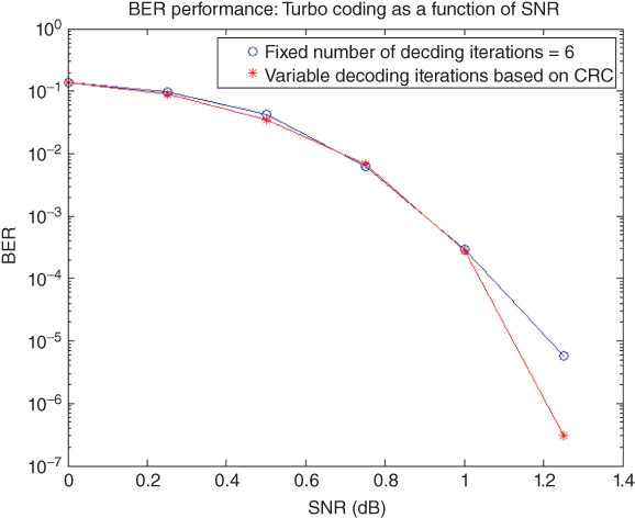
The BER results in Figure 4.6 indicate that we get similar BER performance for the range of SNR values with early termination (trace in red) and without early termination (trace in blue).
Figure 4.6 Comparison of BER results for cases of turbo coding with and without CRC-based early terminations
4.5.3 Timing Measurements
In this experiment, we compare the execution times of a transceiver that employs turbo decoding without a CRC-based early-stopping mechanism (chap4_ex04.m) with those of one that does employ a CRC-based early-stopping mechanism (chap4_ex04_crc.m). The experiment is performed by calling the following MATLAB testbench.
EbNo=1; maxNumErrs=1e7; maxNumBits=1e7;
tic; [a,b]=chap4_ex04(EbNo,maxNumErrs, maxNumBits); toc;
tic; [a,b]=chap4_ex04_crc(EbNo,maxNumErrs, maxNumBits); toc;
The first line of the script forces both transceiver functions to process 10 million bits per call for a given Eb/N0 value of 1 dB. The second line uses the MATLAB functions tic and toc to obtain the elapsed time for an algorithm without early termination. The third line records the elapsed time for an algorithm with early termination.
The results printed in the MATLAB command line are shown in Figure 4.7. It takes considerably less time to process the same number of input frames with early termination (131.27 seconds) than it does without early termination (178.77 seconds).
Figure 4.7 Typical saving in execution time with early-termination turbo decoding

4.6 Rate Matching
So far we have only considered a turbo coding operation with a base coding rate of 1/3. Rate matching is instrumental in the implementation of adaptive coding, an important feature of modern communications standards. It helps augment the throughput based in the channel conditions. In low-distortion channels, we can code the data with coding rates near unity, which reduces the number of bits transmitted for forward error coding. On the other hand, in degraded channels we can use smaller coding rates and increase the number of error-correction bits.
In channel coding with rate matching, we start with a constant 1/3-rate turbo coder and use rate matching to arrive at any desired rate by repeating or puncturing. If a rate lower than 1/3 is requested, we repeat the turbo coder output bits. For rates higher than 1/3, we puncture or remove some of the turbo coder output bits. The puncturing of the code is not the result of simple subsampling but rather is based on an interleaving method. This method is shown to preserve the hamming distances of the resulting higher-rate code 2.
Rate matching is composed of:
- Subblock interleaving
- Parity-bit interlacing
- Bit pruning
- Rate-based bit selection and transmission.
The first operation in rate matching is the subblock interleaving, based on a simple rectangular interleaver. By using a circular buffer concept in rate matching, both the puncturing and the repeating operations that are necessary to increase or decrease (respectively) the rate to the desired level are simply implemented by bit selection operating on a circular buffer. Finally, by concatenating codeblocks, the encoded bits become ready for transfer to the PDSCH for processing.
4.6.1 MATLAB Examples
Staying true to our pedagogic approach of moving from simple to more complex, we will first study rate matching before going on to introduce all the details of transport block channel coding in the LTE standard. This MATLAB function implements the three features of rate matching as specified in the LTE standard: subblock interleaving, Parity bit interlacing, and rate matching with a circular buffer bit selection.
This MATLAB function shows the sequence of interleaving, interlacing, and bit-selection operations that defines the LTE rate-marching algorithm. The input of the rate marcher is the output of a 1/3 turbo encoder. So, for an input block of size K, the input to the rate marcher has a size of 3(K + 4), comprising three streams of Systematic and two Parity streams. First, we subdivide each of the three streams into 32 bit sections and interleave each of these sections. Since each stream may not be divisible by 32, we add dummy bits to the beginnings of the streams, such that the resulting vector can be subdivided into some integer number of 32 bits. The subblock interleavings used for Systematic and Parity 1 bits are the same, but the subblock interleaved for Parity 2 bits is different.
We then create an output vector composed of dummy padded Systematic bits and the interlacing of dummy padded Parity 1 and Parity 2 bits. Finally, by removing the dummy bits, we generate the circular buffer used for the rate-necking operation. The last step in rate matching is a bit selection, where the dummy bits in the circular buffer are removed and the first few bits are selected. The ratio of selected bits to the input length of the turbo encoder is the new rate after rate matching.
function y= RateMatcher(in, Kplus, Rate)
% Rate matching per coded block, with and without the bit selection.
D = Kplus+4;
if numel(in)˜=3*D, error('Kplus (2nd argument) times 3 must be size of input 1.');end
% Parameters
colTcSb = 32;
rowTcSb = ceil(D/colTcSb);
Kpi = colTcSb * rowTcSb;
Nd = Kpi - D;
% Bit streams
d0 = in(1:3:end); % systematic
d1 = in(2:3:end); % parity 1st
d2 = in(3:3:end); % parity 2nd
i0=(1:D)';
Index=indexGenerator(i0,colTcSb, rowTcSb, Nd);
Index2=indexGenerator2(i0,colTcSb, rowTcSb, Nd);
% Sub-block interleaving - per stream
v0 = subBlkInterl(d0,Index);
v1 = subBlkInterl(d1,Index);
v2 = subBlkInterl(d2,Index2);
vpre=[v1,v2].';
v12=vpre(:);
%   Concat 0, interleave 1, 2 sub-blk streams
% Bit collection
wk = zeros(numel(in), 1);
wk(1:D) = remove_dummy_bits( v0 );
wk(D+1:end) = remove_dummy_bits( v12);
% Apply rate matching
N=ceil(D/Rate);
y=wk(1:N);
end
function v = indexGenerator(d, colTcSb, rowTcSb, Nd)
% Sub-block interleaving - for d0 and d1 streams only
colPermPat = [0, 16, 8, 24, 4, 20, 12, 28, 2, 18, 10, 26, 6, 22, 14, 30,…
              1, 17, 9, 25, 5, 21, 13, 29, 3, 19, 11, 27, 7, 23, 15, 31];
% For 1 and 2nd streams only
y = [NaN*ones(Nd, 1); d];       % null (NaN) filling
inpMat = reshape(y, colTcSb, rowTcSb).';
permInpMat = inpMat(:, colPermPat+1);
v = permInpMat(:);
end
function v = indexGenerator2(d, colTcSb, rowTcSb, Nd)
% Sub-block interleaving - for d2 stream only
colPermPat = [0, 16, 8, 24, 4, 20, 12, 28, 2, 18, 10, 26, 6, 22, 14, 30,…
              1, 17, 9, 25, 5, 21, 13, 29, 3, 19, 11, 27, 7, 23, 15, 31];
pi = zeros(colTcSb*rowTcSb, 1);
for i = 1 : length(pi)
    pi(i) = colPermPat(floor((i-1)/rowTcSb)+1) + colTcSb*(mod(i-1, rowTcSb)) + 1;
end
% For 3rd stream only
y = [NaN*ones(Nd, 1); d];       % null (NaN) filling
inpMat = reshape(y, colTcSb, rowTcSb).';
ytemp = inpMat.';
y = ytemp(:);
v = y(pi);
end
function out = remove_dummy_bits( wk )
%UNTITLED5 Summary of this function goes here
%out = wk(find(˜isnan(wk)));
out=wk(isfinite(wk));
end
function out=subBlkInterl(d0,Index)
out=zeros(size(Index));
IndexG=find(˜isnan(Index)==1);
IndexB=find(isnan(Index)==1);
out(IndexG)=d0(Index(IndexG));
Nd=numel(IndexB);
out(IndexB)=nan*ones(Nd,1);
end
In the RateDematcher function we perform the inverse operations to those in the rate matching. We create a vector composed of dummy padded Systematic and Parity bits, place the available samples of the input vectors in the vector, and by de-interlacing and de-interleaving create the right number of LLR samples to become inputs to the 1/3 turbo decoder.
function out = RateDematcher(in, Kplus)
% Undoes the Rate matching per coded block.
%#codegen
% Parameters
colTcSb = 32;
D = Kplus+4;
rowTcSb = ceil(D/colTcSb);
Kpi = colTcSb * rowTcSb;
Nd = Kpi - D;
tmp=zeros(3*D,1);
tmp(1:numel(in))=in;
% no bit selection - assume full buffer passed in
i0=(1:D)';
Index= indexGenerator(i0,colTcSb, rowTcSb, Nd);
Index2= indexGenerator2(i0,colTcSb, rowTcSb, Nd);
Indexpre=[Index,Index2+D].';
Index12=Indexpre(:);
% Bit streams
tmp0=tmp(1:D);
tmp12=tmp(D+1:end);
v0 = subBlkDeInterl(tmp0, Index);
d12=subBlkDeInterl(tmp12, Index12);
v1=d12(1:D);
v2=d12(D+(1:D));
% Interleave 1, 2, 3 sub-blk streams - for turbo decoding
temp = [v0 v1 v2].';
out = temp(:);
end
function v = indexGenerator(d, colTcSb, rowTcSb, Nd)
% Sub-block interleaving - for d0 and d1 streams only
colPermPat = [0, 16, 8, 24, 4, 20, 12, 28, 2, 18, 10, 26, 6, 22, 14, 30,…
              1, 17, 9, 25, 5, 21, 13, 29, 3, 19, 11, 27, 7, 23, 15, 31];
% For 1 and 2nd streams only
y = [NaN*ones(Nd, 1); d];       % null (NaN) filling
inpMat = reshape(y, colTcSb, rowTcSb).';
permInpMat = inpMat(:, colPermPat+1);
v = permInpMat(:);
end
function v = indexGenerator2(d, colTcSb, rowTcSb, Nd)
% Sub-block interleaving - for d2 stream only
colPermPat = [0, 16, 8, 24, 4, 20, 12, 28, 2, 18, 10, 26, 6, 22, 14, 30,…
              1, 17, 9, 25, 5, 21, 13, 29, 3, 19, 11, 27, 7, 23, 15, 31];
pi = zeros(colTcSb*rowTcSb, 1);
for i = 1 : length(pi)
    pi(i) = colPermPat(floor((i-1)/rowTcSb)+1) + colTcSb*(mod(i-1, rowTcSb)) + 1;
end
% For 3rd stream only
y = [NaN*ones(Nd, 1); d];       % null (NaN) filling
inpMat = reshape(y, colTcSb, rowTcSb).';
ytemp = inpMat.';
y = ytemp(:);
v = y(pi);
end
function out=subBlkDeInterl(in,Index)
out=zeros(size(in));
IndexG=find(˜isnan(Index)==1);
IndexOut=Index(IndexG);
out(IndexOut)=in;
end
4.6.2 BER Measurements
We will now examine the effects of using a coding rate other than 1/3 for the turbo coding algorithm. The function chap6_ex05_crc implements the transceiver algorithm that performs a combination of CRC generation, turbo coding, scrambling, and modulation and their inverse operations, while implementing the early-termination mechanism and applying rate-matching operations.
function [ber, numBits, itersHist]=chap6_ex05_crc(EbNo, maxNumErrs, maxNumBits)
%% Constants
FRM=2432-24;                                           % Size of bit frame
Kplus=FRM+24;
Indices = lteIntrlvrIndices(Kplus);
ModulationMode=1;
k=2*ModulationMode;
CodingRate=1/2;
snr = EbNo + 10*log10(k) + 10*log10(CodingRate);
noiseVar = 10.^(-snr/10);
Hist=dsp.Histogram('LowerLimit', 1, 'UpperLimit', maxIter, 'NumBins', maxIter,
'RunningHistogram', true);
%% Processing loop modeling transmitter, channel model and receiver
numErrs = 0; numBits = 0; nS=0;
while ((numErrs < maxNumErrs) && (numBits < maxNumBits))
    % Transmitter
    u  =  randi([0 1], FRM,1);                                                           % Randomly generated input bits
    data= CbCRCGenerator(u);                                                        % Transport block CRC code
    t0 = TurboEncoder(data, Indices);                                              % Turbo Encoder
    t1= RateMatcher(t0, Kplus, CodingRate);                                  % Rate Matcher
    t2 = Scrambler(t1, nS);                                                                % Scrambler
    t3 = Modulator(t2, ModulationMode);                                       % Modulator
    % Channel
    c0 = AWGNChannel(t3, snr);                                                      % AWGN channel
    % Receiver
    r0 = DemodulatorSoft(c0, ModulationMode, noiseVar);            % Demodulator
    r1 = DescramblerSoft(r0, nS);                                                     % Descrambler
    r2 = RateDematcher(r1, Kplus);                                                  % Rate Matcher
    [y, ˜, iters]  = TurboDecoder_crc(-r2, Indices);                         % Turbo Decoder
    % Measurements
    numErrs     = numErrs + sum(y˜=u);                                           % Update number of bit errors
    numBits     = numBits + FRM;                                                     % Update number of bits processed
    itersHist    =  step(Hist, iters);                                                    % Update histogramof iteration numbers
    % Manage slot number with each subframe processed
    nS = nS + 2; nS = mod(nS, 20);
end
%% Clean up & collect results
ber = numErrs/numBits;                                          % Compute Bit Error Rate (BER)
By adding the rate-matching operation after the turbo encoder and the rate-dematching operation after the decoder we can simulate the effects of using any coding rate higher than 1/3. Of course, lower coding rates are used in transmission scenarios dealing with cleaner channels, where less error correction is desirable.
By modifying the variable CodingRate in the function, we activate the rate-matching operations and can examine the BER performance as a function of SNR for multiple values of target coding rates. The results in Figure 4.8 show that, as expected, the performance of a 1/3-rate transceiver is superior to that of the ½ transceiver.
Figure 4.8 Effect of rate matching on turbo coding BER performance

4.7 Codeblock Segmentation
In LTE, a transport block connects the MAC layer and the PHY. The transport block usually contains a large amount of data bits, which are transmitted at the same time. The first set of operations performed on a transport block is channel coding, which is applied to each codeblock independently. If the input frame to the turbo encoder exceeds the maximum size, the transport block is usually divided into multiple smaller blocks known as codeblocks. Since the internal interleaver of the turbo encoder is only defined for 188 input block sizes, the sizes of these codeblocks need to match the set of codeblock sizes supported by the turbo coder. A combination of codeblock CRC attachment, turbo coding, and rate matching is then applied to each codeblock independently.
4.7.1 MATLAB Examples
In the following segmentation function we search for the best subblock size to satisfy two properties: (i) it is one among 188 valid block sizes; and (ii) it is an exact integer multiple of the subblock size. The number of subblocks contained in a codeblock is known as parameter C and the size of each subblock is known as Kplus. We also need to compute a parameter E for the codeword. The output of channel coding is known as the codeword; the size of the codeword is the product of C subblocks and the output size per subblock E. The total codeword size is determined by the scheduler, depending on the number of available resources. The effective coding rate is then the ratio of codeword size to subblock size.
function  [C, Kplus] = CblkSegParams(tbLen)
%#codegen
%% Code block segmentation
blkSize = tbLen + 24;
maxCBlkLen = 6144;
if (blkSize <= maxCBlkLen)
    C = 1;          % number of code blocks
    b = blkSize;    % total bits
else
    L = 24;
    C = ceil(blkSize/(maxCBlkLen-L));
    b = blkSize + C*L;
end
% Values of K from table 5.1.3-3
validK = [40:8:512 528:16:1024 1056:32:2048 2112:64:6144].';
% First segment size
temp = find(validK >= b/C);
Kplus = validK(temp(1), 1);     % minimum K
The following MATLAB function calculates the sizes of subblocks and determines how many are processed in parallel to reconstitute the channel coding outputs. First we divide the total number of codeword bits by the number of subblocks. For each subblock, we ensure that the number of output bits is divisible by the number of modulation bits and the resulting number of multi-antenna layers.
function E = CbBitSelection(C, G, Nl, Qm)
%#codegen
% Bit selection parameters
% G = total number of output bits
% Nl   Number of layers a TB is mapped to (Rel10)
% Qm    modulation bits
Gprime = G/(Nl*Qm);
gamma = mod(Gprime, C);
E=zeros(C,1);
% Rate matching with bit selection
for cbIdx=1:C
        if ((cbIdx-1) <= (C-1-gamma))
            E(cbIdx) = Nl*Qm*floor(Gprime/C);
        else
             E(cbIdx)   = Nl*Qm*ceil(Gprime/C);
        end
end
In the receiver, in order to correctly perform the inverse of matching operations, we need the parameters C and Kplus (the number of subblocks and the size of each subblock, respectively).
4.8 LTE Transport-Channel Processing
Figure 4.9 shows a block diagram of TrCH processing. Five functional components characterize transport block processing:
- Transport-block CRC attachment
- Codeblock segmentation and codeblock CRC attachment
- Turbo coding based on a 1/3 rate
- Rate matching to handle any requested coding rates
- Codeblock concatenation.
Figure 4.9 Structure of transport-channel processing
4.8.1 MATLAB Examples
In the following MATLAB function, we need to distinguish between the case where the transport contains only a single codeblock and the cases where it contains more than one codeblock, since in the first case we do not need to apply the CRC attachment to the codeblock as the transport block already contains a CRC attachment.
function [out, Kplus, C] = TbChannelCoding(in, prmLTE)
% Transport block channel coding
%#codegen
inLen = size(in, 1);
[C, ˜, Kplus] =  CblkSegParams(inLen-24);
intrlvrIndices = lteIntrlvrIndices(Kplus);
G=prmLTE.maxG;
E_CB=CbBitSelection(C, G, prmLTE.NumLayers, prmLTE.Qm);
% Initialize output
out = false(G, 1);
% Channel coding the TB
if (C==1) % single CB, no CB CRC used
    % Turbo encode
    tEncCbData = TurboEncoder( in, intrlvrIndices);
    % Rate matching, with bit selection
    rmCbData =  RateMatcher(tEncCbData, Kplus,  G);
    % unify code paths
    out = logical(rmCbData);
else % multiple CBs in TB
    startIdx = 0;
    for cbIdx = 1:C
        % Code-block segmentation
        cbData = in((1:(Kplus-24)) + (cbIdx-1)*(Kplus-24));
        % Append checksum to each CB
        crcCbData = CbCRCGenerator( cbData);
        % Turbo encode each CB
        tEncCbData = TurboEncoder(crcCbData, intrlvrIndices);
        % Rate matching with bit selection
        E=E_CB(cbIdx);
        rmCbData = RateMatcher(tEncCbData, Kplus,  E);
        % Code-block concatenation
        out((1:E) + startIdx) = logical(rmCbData);
        startIdx = startIdx + E;
    end
end
The sequence of operations performed in channel decoding can be regarded as the inverse of those performed in channel coding, as follows:
- Iteration over each codeblock
- Rate dematching (from target rate to 1/3 rate) composed of:
- Bit selection and insertion
- Parity-bit deinterlacing
- Subblock deinterleaving
- Recovery of Systematic and Parity bits for turbo decoding
- Codeblock 1/3-rate turbo decoding with early termination based on CRC.
Here we are using CRC of the entire transport block as another early stopping criterion and as a mechanism for updating the state of HARQ. The following MATLAB function summarizes the operations in the TrCH decoder.
function [decTbData, crcCbFlags, iters] = TbChannelDecoding( in, Kplus, C, prmLTE)
% Transport block channel decoding.
%#codegen
intrlvrIndices = lteIntrlvrIndices(Kplus);
% Make fixed size
G=prmLTE.maxG;
E_CB=CbBitSelection(C, G, prmLTE.NumLayers, prmLTE.Qm);
% Channel decoding the TB
if (C==1)   % single CB, no CB CRC used
    % Rate dematching, with bit insertion
    deRMCbData = RateDematcher(-in, Kplus)
    % Turbo decode the single CB
    tDecCbData =TurboDecoder(deRMCbData, intrlvrIndices,  prmLTE.maxIter)
    % Unify code paths
    decTbData  = logical(tDecCbData);
else % multiple CBs in TB
    decTbData  = false((Kplus-24)*C,1); % Account for CB CRC bits
    startIdx = 0;
    for cbIdx = 1:C
        % Code-block segmentation
        E=E_CB(cbIdx);
        rxCbData = in(dtIdx(1:E) + startIdx);
        startIdx = startIdx + E;
        % Rate dematching, with bit insertion
        %   Flip input polarity to match decoder output bit mapping
        deRMCbData = lteCbRateDematching(-rxCbData, Kplus, C, E);
        % Turbo decode each CB with CRC detection
        %   - uses early decoder termination at the CB level
        [crcDetCbData, crcCbFlags(cbIdx), iters(cbIdx)] = …
                    TurboDecoder_crc(deRMCbData, intrlvrIndices);
        % Check the crcCBFlag per CB. If still in error, abort further TB
        % processing for remaining CBs in the TB, as the HARQ process will
        % request retransmission for the whole TB.
        if (˜prmLTE.fullDecode)
            if (crcCbFlags(cbIdx)==1) % error
                break;
            end
        end
        % Code-block concatention
        decTbData((1:(Kplus-24)) + (cbIdx-1)*(Kplus-24)) = logical(crcDetCbData);
    end
end
4.8.2 BER Measurements
We now measure the bit-error rates of the LTE downlink TrCH in the presence of the AWGN channel noise. The function chap4_ex06 combines all the TrCH processing operations with scrambling and modulation.
function [ber, numBits]=chap4_ex06(EbNo, maxNumErrs, maxNumBits)
%% Constants
FRM=2432-24;
Kplus=FRM+24;
Indices = lteIntrlvrIndices(Kplus);
ModulationMode=1;
k=2*ModulationMode;
maxIter=6;
CodingRate=1/2;
snr = EbNo + 10*log10(k) + 10*log10(CodingRate);
noiseVar = 10.^(-snr/10);
%% Processing loop modeling transmitter, channel model and receiver
numErrs = 0; numBits = 0; nS=0;
while ((numErrs < maxNumErrs) && (numBits < maxNumBits))
    % Transmitter
    u  =  randi([0 1], FRM,1);                                                           % Randomly generated input bits
    data= CbCRCGenerator(u);                                                        % Transport block CRC code
    [t1, Kplus, C] = TbChannelCoding(data,Indices,maxIter);          % TransportChannel encoding
    t2 = Scrambler(t1, nS);                                                                % Scrambler
    t3 = Modulator(t2, ModulationMode);                                       % Modulator
    % Channel
    c0 = AWGNChannel(t3, snr);                                                      % AWGN channel
    % Receiver
    r0 = DemodulatorSoft(c0, ModulationMode, noiseVar);            % Demodulator
    r1 = DescramblerSoft(r0, nS);                                                     % Descrambler
     [r2,˜,˜] = TbChannelDecoding(r1, Kplus, C, Indices,maxIter);  % Transport Channel decoding
    y   =  CbCRCDetector(r2);                                                           % Code block CRC detector
    % Measurements
    numErrs     = numErrs + sum(y˜=u);                                           % Update number of bit errors
    numBits     = numBits + FRM;                                                     % Update number of bits processed
    % Manage slot number with each subframe processed
    nS = nS + 2; nS = mod(nS, 20);
end
%% Clean up & collect results
ber = numErrs/numBits;                                          % Compute Bit Error Rate (BER)
By executing this function with a range of SNR values, we can verify that the combination of processing applied to the DLSCH and PDSCH without OFDM and MIMO operations is implemented properly. Figure 4.10 illustrates the BER performance of the transceiver. In this experiment, we use rate matching with a coding rate of 1/2 and a QPSK modulator and repeat the operations for a range of values for a maximum number of iterations from one to six. As expected, by providing more decoding iterations we obtain progressively better performance results. This again shows the critical role that early termination can play in making the DLSCH processing specified in the LTE standard more realizable.
Figure 4.10 BER performance of DLSCH and QPSK as a function of Eb/N0 and the number of decoding operations

4.9 Chapter Summary
So far we have studied the forward error-correction scheme employed in the LTE standard based on a simple channel model (AWGN). The LTE standard uses AWGN environment propagation for static performance measurement. No fading or multipaths exist for this propagation model and it does not take into account the frequency response of real channels. Most real channels add to the transmitted signal various forms of fading and other correlated distortions. These fading profiles introduce intersymbol interference, which must be compensated by using equalization.
We observe that the performance of iterative turbo channel coding depends on the number of iterations used. This motivates the discussion regarding simulation acceleration in Chapter 9. We also note that studying the performance in an AWGN channel ignores real channel models and the effects of multipath fading. This motivates the discussions in Chapters 5 and 6 on how to combat multipath fading using OFDM and Single-Carrier Frequency Division Multiplexing (SC-FDM) with frequency-domain equalizers.
References
[1] 3GPP (2009) Evolved Universal Terrestrial Radio Access (E-UTRA); Multiplexing and Channel Coding. TS 36.212.
[2] Proakis, J. and Salehi, M. (2007) Digital Communications, 5th edn, McGraw-Hill Education, New York.
[3] 3GPP (2011) Evolved Universal Terrestrial Radio Access (E-UTRA); Physical Channels and Modulation Version 10.0.0. TS 36.211, January 2011.
[4] Online: http://www.mathworks.com/help/comm/ug/define-basic-system-objects-1.html (last accessed September 30, 2013).