
Chapter 5
OFDM
So far we have considered the modulation, scrambling, and coding specifications of the LTE standard and have used a simplistic channel model (Additive White Gaussian Noise, AWGN) to undertake performance evaluations. Understanding of Orthogonal Frequency Division Multiplexing (OFDM), which is the fundamental air interface in the standard, necessitates understanding and modeling of more sophisticated channel models.
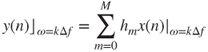
In this chapter we consider realistic channel models that take into account the dynamic channel responses and fading conditions. Short-term fading effects such as multipath fading and Doppler effects resulting from mobility will lead to frequency-selective channel models. OFDM and Single-Carrier Frequency Division Multiplexing (SC-FDM) multiple-access technologies in LTE, for downlink and uplink respectively, use efficient frequency-domain equalizers to combat frequency-selective fading and contribute to its superior spectral efficiency. In this chapter we will focus on a single-antenna configuration, while in the next chapter we will combine Multiple Input Multiple Output (MIMO) and OFDM.
We will detail the basis of the OFDM technology and discuss OFDM frame structure and implementation in the LTE standard. We will then discuss the time–frequency mapping of the OFDM signal and the various resource element granularities used to adaptively exploit the channel bandwidth, followed by the frequency-domain equalization of the OFDM signal at the receiver. We examine Zero Forcing (ZF), Minimum Mean Squared Error (MMSE), equalizers and details of the interpolation of reference signals or pilots. Finally, we examine the performance of a transceiver composed of components developed so far under various multipath fading and mobility conditions specified by the standard.
5.1 Channel Modeling
Wireless channels are characterized by the availability of different paths of propagation between transmitters and receivers. Besides the direct path between the transmitter and the receiver, which may even not exist, other paths can be formed through reflection, diffraction, scattering, or other propagation scenarios. By going through different paths, different versions of the transmitted signals can be received simultaneously at the receiver. These different versions exhibit varying profiles of signal power and time delay or phase. Since these received signals are correlated in time, an AWGN model is not the most representative channel model for most wireless connections. Therefore, proper modeling of the characteristics of a wireless channel is an important requirement for the design of mobile communications systems. Channel propagation usually results in a reduced power in received signals relative to the transmitted signal. In general, the power reductions are treated in two categories: (i) signal attenuations or large-scale fading and (ii) fading or small-scale fading.
5.1.1 Large-Scale and Small-Scale Fading
Path loss and shadowing are among the most prominent large-scale fading effects. These large-scale features are taken into account in design and cellular topography 1. Small-scale fading includes multipath fading and time dispersion due to mobility. These features are of short duration and must be adaptively dealt with. The design of the PHY (Physical Layer) should include techniques that effectively deal with these types of channel impairment 1.
5.1.2 Multipath fading Effects
Multipath fading is characterized by a power-delay profile comprising two components: a vector of relative delays and a vector of average power parameters. Another useful set of scalar measures is either mean excess delay or the Root Mean Square (RMS) delay spread as the first and second moments of relative delays. Multipath fading can be flat or frequency-selective. If the bandwidth is larger than the inverse of the delay spread, channel frequency response will lead to multipath fading.
In the cellular communication context, signals are received at the mobile terminal following a direct path from the base station. Some signals will also be reflected off buildings or other reflectors and will reach the mobile terminal with a time delay and an attenuated power. Since the mobile receiver gets the linear combination of these signals, the net signal obtained is essentially a convolution of input signal and the impulse response of the channel. In the frequency domain, the frequency response of the channel includes different response patterns at different frequencies; we thus have frequency-selective fading (Figure 5.1).
Figure 5.1 Multipath propagation, frequency-selective fading, and frequency-domain equalization

In the case of a time-dispersive channel with multipath-propagation characteristics, there will be not only intersymbol interference within a subcarrier but also interference between subcarriers. This is because the orthogonality between the subcarriers will be partially lost due to the overlap of the demodulator correlation interval for one path with the symbol boundary of another. The integration interval, used to compute the Fast Fourier Transform (FFT), will not necessarily correspond to an integer number of periods of complex exponentials of that path, as the modulation symbols may differ between consecutive symbol intervals.
5.1.3 Doppler Effects
For mobile systems transmitting over a broad bandwidth, such as the LTE, the predominant channel degradation is a result of short-term fading caused by multipath propagation. We need to account for the effects of a fading channel in order to provide an accurate evaluation of the LTE system performance. As a result of mobile terminal movement, the profile of channel impulse response can vary. Fast- and slow-fading channels reflect the speed of the mobile terminal and are expressed in terms of Doppler frequency shifts 1.
5.1.4 MATLAB® Examples
We can study the effects of channel responses to a transmitted signal by using the various channel models of the Communications System Toolbox. Rayleigh and Rician channel objects can be used to model a single propagation path and the comm.MIMOChannel System object can be used to study the effects of multiple antennas and multiple propagation paths. All of these components use the delay profile and Doppler shift as parameters to model the dynamics of a fading channel.
In order to become familiar with these objects, let us examine four types of channel separately. The differences between these channel models relate to (i) whether or not a frequency-flat or a frequency-selective channel is present and (ii) whether or not a frequency-dispersive channel is present due to the Doppler shift caused by the mobility of the receiver.
5.1.4.1 Low-Mobility Flat-Fading Channels
The first type of channel is a low-mobility flat-fading channel. In this case, the delay profile does not contain multiple shifts in time. It is characterized by a single dominant delay value that denotes the time difference between the transmitter and the receiver. Furthermore, low mobility leads to a Doppler shift of near zero. The following MATLAB function implements such a channel model.
function y = ChanModelFading(in, Chan)
% Static (No mobility) Flat Fading Channel
%#codegen
% Get simulation params
numTx=1;
numRx=1;
chanSRate = Chan.chanSRate;
PathDelays = Chan.PathDelays;
PathGains  = Chan.PathGains;
Doppler      = Chan.DopplerShift;
% Initialize objects
persistent chanObj
if isempty(chanObj)
    chanObj = comm.MIMOChannel(…
        'SampleRate', chanSRate, …
        'MaximumDopplerShift', Doppler, …
        'PathDelays', PathDelays,…
        'AveragePathGains', PathGains,…
        'NumTransmitAntennas', numTx,…
        'TransmitCorrelationMatrix', eye(numTx),…
        'NumReceiveAntennas', numRx,…
        'ReceiveCorrelationMatrix', eye(numRx),…
        'PathGainsOutputPort', false,…
        'NormalizePathGains', true,…
        'NormalizeChannelOutputs', true);
end
y = step(chanObj, in);
In order to visualize the effect of this type of channel on a system, we add the fading channel to a system containing coding scrambling and modulation and observe the input signal to the demodulator. Note that by running the experiment in the following MATLAB function, we can observe how even a static flat-fading channel that represents a mild form of channel response significantly degrades the performance.
function [ber, bits] = chap5_ex01(EbNo, maxNumErrs, maxNumBits, prmLTE)
%#codegen
%% Constants
FRM=2432-24;
Kplus=FRM+24;
Indices = lteIntrlvrIndices(Kplus);
ModulationMode=1;
k=2*ModulationMode;
maxIter=6;
CodingRate=1/2;
snr = EbNo + 10*log10(k) + 10*log10(CodingRate);
noiseVar = 10.^(-snr/10);
%% Processing loop modeling transmitter, channel model and receiver
numErrs = 0; numBits = 0; nS=0;
while ((numErrs < maxNumErrs) && (numBits < maxNumBits))
    % Transmitter
    u  =  randi([0 1], FRM,1);                                                           % Randomly generated input bits
    data= CbCRCGenerator(u);                                                        % Transport block CRC code
    [t1, Kplus, C] = TbChannelCoding(data, prmLTE);
    t2 = Scrambler(t1, nS);                                                                % Scrambler
    t3 = Modulator(t2, ModulationMode);                                       % Modulator
    % Channel & Add AWG noise
    [rxFade, ˜] = MIMOFadingChan(t3, prmLTE);
    nVar = 10.^(0.1.*(-EbNo));                                                          % assume unit sigPower
    c0  = AWGNChannel2(rxFade, nVar );                                          % AWGN channel
    % Receiver
    r0 = DemodulatorSoft(c0, ModulationMode, noiseVar);            % Demodulator
    r1 = DescramblerSoft(r0, nS);                                                     % Descrambler
    r2 = RateDematcher(r1, Kplus);                                                  % Rate Matcher
    r3  = TurboDecoder(-r2, Indices,  maxIter);                                % Turbo Decoder
    y   =  CbCRCDetector(r3);                                                           % Code block CRC detector
    % Measurements
    numErrs     = numErrs + sum(y˜=u);                                           % Update number of bit errors
    numBits     = numBits + FRM;                                                     % Update number of bits processed
    % Manage slot number with each subframe processed
    nS = nS + 2; nS = mod(nS, 20);
end
%% Clean up & collect results
ber = numErrs/numBits;                                          % Compute Bit Error Rate (BER)
Figure 5.2 shows the frequency response of the transmitted and received signals within the transmission bandwidth. It explains why this is called a flat-fading channel, as throughout the bandwidth at each frequency the response is faded by the same value.
Figure 5.2 Low-mobility flat-fading channel

5.1.4.2 High-Mobility Flat-Fading Channels
We now set a non-zero value for the Doppler shift in order to model a high-mobility flat-fading channel. Note that the profile of the channel response is still that of flat fading, but the gain for the entire spectrum varies as a function of time. Also, the constellation of the received signal still resembles a 64QAM (Quadrature Amplitude Modulation) modulation. However, at each time step the constellation rotates based on the phase offset as a result of the Doppler shift. These effects are illustrated in Figure 5.3.
Figure 5.3 High-mobility flat-fading channel

5.1.4.3 Low-Mobility Frequency-Selective Channels
In this section, we examine a frequency-selective channel model that will still have a zero Doppler shift but it will have a vector for the associated delay profile. With the vector of time delays, we observe a gain vector of the same size. This results in a frequency-selective channel response, as observed in Figure 5.4.
Figure 5.4 Low-mobility frequency-selective fading

5.1.4.4 High-Mobility Frequency-Selective Channels
Finally, by setting a non-zero value for the Doppler shift we can model a high-mobility frequency-selective channel. As in the previous high-mobility case, we observe a varying profile for channel gain at different frequency values. We also note that the channel responses vary in time. Figure 5.5 illustrates the magnitude spectra of the channel response computed over two subframes 10 ms apart.
Figure 5.5 High-mobility frequency-selective fading

5.2 Scope
In this book, without any loss for generality, we focus on the normal Cyclic Prefix (CP) that leads to a particular time framing (seven OFDM symbols per slot) and subcarrier spacing of 15 kHz. The MATLAB functionality is flexibly parameterized such that by changing a few parameters, extended CP mode can be easily simulated.
In this volume we do not deal with system access procedures, startup, random access, or handoff scenarios. We discuss the steady-state signal processing downlink transmission that takes place once the call within a cell is already established. As such, the synchronization signals and the Broadcast Channels (BCHs) (downlink) and random access channels (uplink) will not be elaborately discussed and the accompanying MATLAB functions will not be developed.
5.3 Workflow
Starting with coding, modulation, and scrambling, we add channel modeling, which includes flat or frequency-selective fading. In this chapter we discuss a single-antenna transmission scenario (either Single Input Single Output, SISO, or Single Input Multiple Output, SIMO). We focus on reference-signal generation, resource-grid specification, and OFDM transmission. Finally, we put together the testbench for the system model that implements the first mode of downlink transmission.
5.4 OFDM and Multipath Fading
The OFDM modulated signal is computed as the Inverse Fast Fourier Transform (IFFT) of the resource elements associated with different subcarriers. The IFFT output can be considered the sum of complex exponential functions known as basis functions, complex sinusoids, harmonics, or tones of a multitone signal. Let us consider one of these tones or harmonics (i.e., the complex exponential associated with a particular subcarrier) as:
5.1 ![]()
Equation 5.2 shows how a channel with an impulse response ![]() operates on the transmitted signal
operates on the transmitted signal ![]() to provide the received signal
to provide the received signal ![]() .
.

Now, due to linearity, when the OFDM signal is subject to a multipath fading channel each of its complex exponential components is also subject to the same channel model. Therefore, we can compute the received version of each subcarrier component of the OFDM signal ![]() as the convolution of that transmitted component and the channel impulse response.
as the convolution of that transmitted component and the channel impulse response.
The next step explains the necessity of introducing the CP to the OFDM formulation. We can substitute the expression ![]() for the complex sinusoidal component in Equation 5.3 if and only if the multipath delay values
for the complex sinusoidal component in Equation 5.3 if and only if the multipath delay values ![]() are less than or equal to the CP length. Otherwise, with even a single delay value outside the CP range, we cross the OFDM symbol boundary and the orthogonality between subcarrier components is lost. Now, assuming that the delay spread is within the CP range, we can obtain the following expression for the received subcarrier component as a function of the transmitted subcarrier component:
are less than or equal to the CP length. Otherwise, with even a single delay value outside the CP range, we cross the OFDM symbol boundary and the orthogonality between subcarrier components is lost. Now, assuming that the delay spread is within the CP range, we can obtain the following expression for the received subcarrier component as a function of the transmitted subcarrier component:
5.4 
After some algebraic simplifications, the output can be expressed as:

Note that the last expression, ![]() , is not a function of the time index n but rather can be viewed as a gain that is a function of the subcarrier index k and is applied to complex exponential component. By defining this gain as
, is not a function of the time index n but rather can be viewed as a gain that is a function of the subcarrier index k and is applied to complex exponential component. By defining this gain as ![]() and substituting it into Equation 5.5, we obtain the following expression for the received OFDM signal component:
and substituting it into Equation 5.5, we obtain the following expression for the received OFDM signal component:
5.6 ![]()
Now we look at OFDM operations at the receiver. Note that after removing the CP, the first operation in the receiver is to compute the Fourier transform, as defined by the following expression:
5.7 
When we the express the received signal based on its Fourier formulation, ![]() , all inner product terms for the frequencies other than the subcarrier vanish due to the orthogonality of the IFFT basis functions. The only non-zero term that determines the Fourier transform of the received signal at the subcarrier belongs to the received subcarrier component; that is:
, all inner product terms for the frequencies other than the subcarrier vanish due to the orthogonality of the IFFT basis functions. The only non-zero term that determines the Fourier transform of the received signal at the subcarrier belongs to the received subcarrier component; that is:
5.8 
By substituting the expression for the received OFDM signal component, we obtain the following:
5.9 
Simplification of this expression results in an intuitive formula for the received signal at a given subcarrier component:
5.10 ![]()
This expression indicates that the received signal at any subcarrier is the product of the transmitted symbol ![]() and the multipath gain
and the multipath gain ![]() . This simple expression is the basis for defining frequency-domain equalization using the pilot signals.
. This simple expression is the basis for defining frequency-domain equalization using the pilot signals.
5.5 OFDM and Channel-Response Estimation
Each transmitted signal component that is subject to the multipath fading channel will arrive at the receiver as a scaled version of the transmitted signal. The gain is characterized by the channel response. Pilot or reference signals can be considered known signals placed at regular subcarriers positions. We can estimate the channel response at those subcarriers by dividing the received version at the subcarrier by the known transmitted value. The channel response at each particular subcarrier is then calculated as:
5.11 
Through various forms of interpolation we can now estimate the channel response not only at known subcarriers but at all subcarriers. This enables us to perform equalization, defined as reversing the effects of the fading channel in the frequency domain. This is more efficient than classical time-domain equalization techniques, which estimate the channel impulse response and use adaptive filtering to equalize the received signals.
5.6 Frequency-Domain Equalization
One of the most important features of the OFDM is its robust and efficient treatment of multipath fading. OFDM compensates for the effect of fading through a frequency-domain approach to equalization. Instead of filtering the received signal in time with the inverse of the channel impulse response, OFDM first constructs a frequency-domain representation of the data and then uses reference signals to invert the frequency response of the channel.
This implies a two-step process. First, the construction of a time–frequency resource grid, where data are aligned with subcarriers in the frequency domain before a series of OFDM symbols is generated in time. This step is also known as the resource element mapping. The types of signal that form the LTE downlink resource grid include the following:
- User data (Physical Downlink Shared Channel, PDSCH)
- Cell-Specific Reference (CSR) signals (otherwise known as pilots)
- Primary Synchronization Signals (PSSs) and Secondary Synchronization Signals (SSSs)
- Physical Broadcast Channels (PBCHs)
- Physical Downlink Control Channels (PDCCHs).
Second, we take the vector of resource elements as input and generate the OFDM symbols. This process involves performing an IFFT operation to generate the OFDM modulated signal and a CP insertion. The use of CP enables the receiver to sample each OFDM symbol for exactly one period in the time domain. The availability of CP helps mitigate the effects of intersymbol interference when the channel delay spread is less than the length of the CP.
Before OFDM signal generation, we need to generate the resource grid based on either a type-1 or a type-2 frame structure. Since we are showcasing Frequency Division Duplex (FDD) duplexing throughout this book, we will use type 1 here. Next we will show how to generate relevant signals to form the resource grid and how to create the OFDM symbols for transmission.
5.7 LTE Resource Grid
Understanding the time–frequency representation of data, organized as the resource grid, is a key step in understanding the LTE transmission scheme. The resource grid is essentially a matrix whose elements are the modulated symbols computed as the outputs of the modulation mapper. In its 2D representation, the y-axis of the grid represents the subcarriers aligned along the frequency dimension and the x-axis represents the OFDM symbols aligned along the time dimension 2.
The placement of data within the resource grid is quite important and reveals some of the design parameters of the LTE physical model. For example, the placement and resolution of pilot signals (CSR) along both axes of the resource grid determines the accuracy of the channel-response estimation in both time and frequency. Similarly, placing the PDCCH control-channel information at the beginning of each subframe helps the receiver decipher important processing parameters (such as the type of modulator and the MIMO mode used) before the system starts decoding the user data in the subframe.
The details involved in placing data within the resource grid can only be understood within the context of time framing and the way in which LTE defines a frame, a subframe, and a slot. Each LTE frame has a duration of 10 ms and is composed of ten 1 ms subframes marked by indices 0 to 9. Each subframe is subdivided into two slots of 0.5 ms duration, with each slot comprising seven OFDM symbols if a normal CP is used and six if an extended CP is used.
The placement of each modulated data type (user data, CSR, DCI, PSS, SSS, and BCH) into the resource grid follows a particular structure in both time and frequency. This structure depends on three parameters: the subcarrier (y-axis) index, the OFDM symbol (x-axis) index, and the index of the 1 ms subframe within a 10 ms frame. All subframes within a frame contain three types of data: user data (PDSCH), pilot CSRs, and downlink control data (PDCCH). The PSS and SSS are only available in subframes 0 and 5 at specific OFDM symbol indices (SSS at fifth symbol and PSS at sixth symbol) and specific subcarrier indices (72 subcarriers around the center of the resource grid). The PBCH is located only within subframe 0 at specific OFDM symbol indices (extending from the seventh to the tenth symbol) and specific subcarrier indices (72 subcarriers around the center of the resource grid). Figure 5.6 illustrates the placement of different modulated data, based on the signal types, within the resource grid.
Figure 5.6 LTE resource grid content – entire grid view – featuring six types of signal

5.8 Configuring the Resource Grid
Let us discuss the size and composition of the resource grid and how it is updated every subframe. Throughout this book, we process the LTE transceiver (transmitter, channel model, and receiver) one subframe at a time. Since the length of each subframe is 1 ms, processing one second of data involves processing 1000 iterations of the transceiver.
In each subframe, the size of the resource grid (![]() = the total number of symbols that fill up the grid) is a function of the following four parameters:
= the total number of symbols that fill up the grid) is a function of the following four parameters:

The total resource grid size is the product of the number of rows (total number of subcarriers) and number of columns (total number of OFDM symbols per subframe). The total number of subcarriers is the product of the number of resource blocks ![]() and number of subcarriers per resource block
and number of subcarriers per resource block ![]() . The total number of OFDM symbols per subframe is the product of the number of symbols per slot
. The total number of OFDM symbols per subframe is the product of the number of symbols per slot ![]() and number of slots per subframe
and number of slots per subframe ![]() .
.
5.12 ![]()
The number of slots per subframe ![]() is a constant value of 2. The number of symbols per slot
is a constant value of 2. The number of symbols per slot ![]() depends on whether a normal or an extended CP is used. As throughout this book we will be using a normal CP, the number of symbols per slot will have a constant value of 7. The number of subcarriers per resource block
depends on whether a normal or an extended CP is used. As throughout this book we will be using a normal CP, the number of symbols per slot will have a constant value of 7. The number of subcarriers per resource block ![]() also depends on CP type; if we assume a normal CP, it has a constant value of 12. Therefore, the resource grid size completely depends on the number of resource blocks, which is a direct function of the bandwidth.
also depends on CP type; if we assume a normal CP, it has a constant value of 12. Therefore, the resource grid size completely depends on the number of resource blocks, which is a direct function of the bandwidth.
As discussed in the last section, the resource elements come from six types of data source: user data, CSR, DCI, PSS, SSS, and BCH. Some of these sources are available in all subframes of a frame (user data, CSR, DCI), some are only available in subframes 0 and 5 (PSS and SSS), and some are only available in subframe 0 (BCH). Since the total number of symbols in a resource grid is constant, in each frame we must compute the amount of user data in three different ways:
Figure 5.7 illustrates the relative locations of six different types of data within the resource grid and focuses on six resource blocks in the center of the grid, where PSS, SSS, and BCH are available in select subframes.
Figure 5.7 LTE resource grid content – focused on eight resource blocks around the center (DC subcarrier) – featuring six different types of data

5.8.1 CSR Symbols
In addition, CSRs are placed throughout each resource block in each subframe with a specific pattern of time and frequency separations. In the single-antenna configuration, LTE specifies two CSR symbols per resource block in each of the four OFDM symbols {0, 5, 7, 12} in any subframe. In OFDM symbols 0 and 7, the starting indices are the first subcarrier, whereas in symbolks 5 and 12 the starting index is the fourth subcarrier. The separation between two CSR symbols in the frequency domain is six subcarriers. There are a total of ![]() CSR symbols available in the resource grid.
CSR symbols available in the resource grid.
5.8.2 DCI Symbols
The DCI is placed within the first N OFDM symbols in each subframe, where N is either 1, 2, or 3. The DCI carries the content of the PDCCH, PCFICH (Physical Control Format Indicator Channel), and PHICH (Physical Hybrid ARQ Indicator Channel), and together these occupy all the resource elements of the first and possibly the second and third OFDM symbols in each subframe, with the exception of the CSR data, which are distributed along the first OFDM symbol of each subframe. The size of the DCI per subframe is ![]() . In this chapter we will not generate and fill in the DCI in the resource grid; we will discuss the DCI in some detail in Chapter 7.
. In this chapter we will not generate and fill in the DCI in the resource grid; we will discuss the DCI in some detail in Chapter 7.
5.8.3 BCH Symbols
The PBCH is located within subframe 0 and occupies six central resource blocks from the seventh to the tenth OFDM symbol. Since the seventh OFDM symbol includes CSR symbols, its BCH has a size of only 60 (72 − 2 × 6), whereas in the next three symbols the size is 72. The total BCH size for the whole frame is ![]() 60 + 3 × 72 = 276.
60 + 3 × 72 = 276.
5.8.4 Synchronization Symbols
Both the PSS and the SSS are placed within the six resource blocks centered on the DC subcarrier. The PSS occupies the sixth OFDM symbol and the SSS occupies the fifth symbol in subframes 0 and 5. Since there is no overlap with CSR signals in these symbols, the total number for each of the synchronization signals is ![]() per subframe, and since two subframes per frame contain synchronization signals, the total is 144 for the frame.
per subframe, and since two subframes per frame contain synchronization signals, the total is 144 for the frame.
5.8.5 User-Data Symbols
The total amount of data in the resource grid depends on the number of resource blocks or essentially on the bandwidth. The resource elements come from six types of data source (user data, CSR, DCI, PSS, SSS, and BCH). Therefore, if the bandwidth is constant the resource grid size is constant and is the sum of all these constituents:
5.13 ![]()
The presence or absence of BCH or synchronization signals in a subframe depends on the subframe index. As a result, the size of the user data in a subframe also depends on the subframe index in the following way:
5.14 ![]()
5.15 ![]()
5.16 ![]()
The following MATLAB function performs calculations highlighted above and sets some of the parameters of the PDSCH. The function takes three parameters as its input argument: the channel bandwidth (chanBW), the number of OFDM symbols dedicated to the control channel in each subframe (contReg), and the modulation type used (modType). It computes many parameters used in PDSCH processing, including the details of the resource grid.
function p= prmsPDSCH(chanBW, contReg, modType, varargin)
%  Returns parameter structures for LTE PDSCH simulation.
%
%   Assumes a FDD, normal cyclic prefix, full-bandwidth, single-user
%   SISO or SIMO downlink transmission.
%% PDSCH parameters
switch chanBW
    case 1      % 1.4 MHz
        BW = 1.4e6; N = 128; cpLen0 = 10; cpLenR = 9;
        Nrb = 6; chanSRate = 1.92e6;
    case 2      % 3 MHz
        BW = 3e6; N = 256; cpLen0 = 20; cpLenR = 18;
        Nrb = 15; chanSRate = 3.84e6;
    case 3      % 5 MHz
        BW = 5e6; N = 512; cpLen0 = 40; cpLenR = 36;
        Nrb = 25; chanSRate = 7.68e6;
    case 4      % 10 MHz
        BW = 10e6; N = 1024; cpLen0 = 80; cpLenR = 72;
        Nrb = 50; chanSRate = 15.36e6;
    case 5      % 15 MHz
        BW = 15e6; N = 1536; cpLen0 = 120; cpLenR = 108;
        Nrb = 75; chanSRate = 23.04e6;
    case 6      % 20 MHz
        BW = 20e6; N = 2048; cpLen0 = 160; cpLenR = 144;
        Nrb = 100; chanSRate = 30.72e6;
end
p.BW = BW;                  % Channel bandwidth
p.N = N;                    % NFFT
p.cpLen0 = cpLen0;          % Cyclic prefix length for 1st symbol
p.cpLenR = cpLenR;          % Cyclic prefix length for remaining
p.Nrb = Nrb;                % Number of resource blocks
p.chanSRate = chanSRate;    % Channel sampling rate
p.contReg = contReg;
if nargin> 3, numTx=varargin{4};else numTx=1;end
if nargin> 4, numRx=varargin{5};else numRx=1;end
p.numTx = numTx;
p.numRx = numRx;
p.numLayers = 1;
p.numCodeWords = 1;
% For Normal cyclic prefix, FDD mode
p.deltaF = 15e3;    % subcarrier spacing
p.Nrb_sc = 12;      % no. of subcarriers per resource block
p.Ndl_symb = 7;     % no. of OFDM symbols in a slot
% Actual PDSCH bits calculation - accounting for PDCCH, PBCH, PSS, SSS
numResources = (p.Nrb*p.Nrb_sc)*(p.Ndl_symb*2);
numCSRRE = 2*2*2 * p.Nrb;               % CSR, RE per OFDMsym/slot/subframe per RB
numContRE = (10 + 12*(p.contReg-1))*p.Nrb;
numBCHRE = 60+72+72+72;              % removing the CSR present in 1st symbol
numSSSRE=72;
numPSSRE=72;
numDataRE=zeros(3,1);
% Account for BCH, PSS, SSS and PDCCH for subframe 0
numDataRE(1)=numResources-numCSRRE-numContRE-numSSSRE - numPSSRE-numBCHRE;
% Account for PSS, SSS and PDCCH for subframe 5
numDataRE(2)=numResources-numCSRRE-numContRE-numSSSRE - numPSSRE;
% Account for PDCCH only in all other subframes
numDataRE(3)=numResources-numCSRRE-numContRE;
% Maximum data resources - with no extra overheads (only CSR + data)
p.numResources=numResources;
p.numCSRResources =  numCSRRE;
p.numContRE = numContRE;
p.numBCHRE = numBCHRE;
p.numSSSRE=numSSSRE;
p.numPSSRE=numPSSRE;
p.numDataRE=numDataRE;
p.numDataResources = p.numResources - p.numCSRResources;
% Modulation types , bits per symbol, number of layers per codeword
Qm = 2 * modType;
p.Qm = Qm;
p.numLayPerCW = p.numLayers/p.numCodeWords;
% Maximum data bits - with no extra overheads (only CSR + data)
p.numDataBits = p.numDataResources*Qm*p.numLayPerCW;
numPDSCHBits =numDataRE*Qm*p.numLayPerCW;
p.numPDSCHBits = numPDSCHBits;
p.maxG = max(numPDSCHBits);
In this chapter we omit the generation of DCI, BCH, and synchronization signals. Instead we focus on computing the content of CSR and user-data signals to fill up the resource grid and use OFDM transmission to model transmission mode 1 of the LTE standard.
5.9 Generating Reference Signals
To ensure that the transmitter and receiver can generate the same CSR reference sequence, LTE uses a Gold sequence that is initialized based on parameters that are available at both the transmitter and the receiver. These parameters include the cell identity number (NcellID), the subframe index (nS), the slot index (i), and the index of OFDM symbols containing the CSR in the slot (IIdx).
The function has two input arguments: the subframe index (nS) and the number of transmit antennas (numTx). As we are only modeling the single-antenna case in this chapter, the second parameter is set to a value of 1. As a convenience, we will use the same function in the following chapter, where multiple antennas are present. Based on the Gold sequence and for all available antenna ports, the function will generate the number of CSR values needed to provide a channel estimation. The output variable y is a matrix whose size is equal to the product of the number of rows and the number of columns. The number of rows is the maximum number of CSR signals in the resource grid and the number of columns is the number of transmit antennas. The following MATLAB function shows how each element of the CSR signal is generated.
function y = CSRgenerator(nS, numTx)
%  LTE Cell-Specific Reference signal generation.
%   Section 6.10.1 of 3GPP TS 36.211 v10.0.0.
%   Generate the whole set per OFDM symbol, for 2 OFDM symbols per slot,
%   for 2 slots per subframe, per antenna port (numTx).
%   This fcn accounts for the per antenna port sequence generation, while
%   the actual mapping to resource elements is done in the Resource mapper.
%#codegen
persistent hSeqGen;
persistent hInt2Bit;
% Assumed parameters
NcellID = 0;        % One of possible 504 values
Ncp = 1;            % for normal CP, or 0 for Extended CP
NmaxDL_RB = 100;    % largest downlink bandwidth configuration, in resource blocks
y = complex(zeros(NmaxDL_RB*2, 2, 2, numTx));
l = [0; 4];     % OFDM symbol idx in a slot for common first antenna port
% Buffer for sequence per OFDM symbol
seq = zeros(size(y,1)*2, 1); % *2 for complex outputs
if isempty(hSeqGen)
    hSeqGen = comm.GoldSequence('FirstPolynomial',[1 zeros(1, 27) 1 0 0 1],…
                                'FirstInitialConditions', [zeros(1, 30) 1], …
                                'SecondPolynomial', [1 zeros(1, 27) 1 1 1 1],…
                                'SecondInitialConditionsSource', 'Input port',…
                                'Shift', 1600,…
                                'SamplesPerFrame', length(seq));
    hInt2Bit = comm.IntegerToBit('BitsPerInteger', 31);
end
% Generate the common first antenna port sequences
for i = 1:2 % slot wise
    for lIdx = 1:2 % symbol wise
        c_init = (2^10)*(7*((nS+i-1)+1)+l(lIdx)+1)*(2*NcellID+1) + 2*NcellID + Ncp;
        % Convert to binary vector
        iniStates = step(hInt2Bit, c_init);
        % Scrambling sequence - as per Section 7.2, 36.211
        seq = step(hSeqGen, iniStates);
        % Store the common first antenna port sequences
        y(:, lIdx, i, 1) = (1/sqrt(2))*complex(1-2.*seq(1:2:end), 1-2.*seq(2:2:end));
    end
end
% Copy the duplicate set for second antenna port, if exists
if (numTx>1)
    y(:, :, :, 2) = y(:, :, :, 1);
end
% Also generate the sequence for l=1 index for numTx = 4
if (numTx>2)
    for i = 1:2 % slot wise
        % l = 1
        c_init = (2^10)*(7*((nS+i-1)+1)+1+1)*(2*NcellID+1) + 2*NcellID + Ncp;
        % Convert to binary vector
        iniStates = step(hInt2Bit, c_init);
        % Scrambling sequence - as per Section 7.2, 36.211
        seq = step(hSeqGen, iniStates);
        % Store the third antenna port sequences
        y(:, 1, i, 3) = (1/sqrt(2))*complex(1-2.*seq(1:2:end), 1-2.*seq(2:2:end));
    end
    % Copy the duplicate set for fourth antenna port
    y(:, 1, :, 4) = y(:, 1, :, 3);
end
5.10 Resource Element Mapping
In this section we detail the resource element mapping that places the components of the resource grid in the locations specified in the standard. Mapping is performed essentially by creating indices to the resource grid matrix and placing various information types within the grid. The illustrations of three different types of resource block given in Figures 5.8–5.10 help visualize formulations for these indices. Depending on which subframe is in use, we populate the BCH, PSS, and SSS in either subframe 0 or subframe 5 of the six central resource blocks around the DC subcarrier. The CSRs are placed in symbols 0 and 5 of each slot, with a frequency-domain separation of six subcarriers.
Figure 5.8 Resource element mapping: all resource blocks in subframes 1, 2, 3, 4, 6, 7, 8, and 9 + noncentral resource blocks of subframes 0 and 5. Includes DCI, CSR, and user data

Figure 5.9 Resource element mapping: central resource blocks of subframe 5. Includes PSS, SSS, DCI, CSR, and user data

Figure 5.10 Resource element mapping: central resource blocks of subframe 0. Includes BCH, PSS, SSS, DCI, CSR, and user data

The following MATLAB function shows resource element mapping. Since MATLAB uses a 1-based indexing notation, we generate indices for various elements in the matrix starting from 1 instead of 0, as specified by the standard. The function takes as input the user data (in), CSR signal (csr), subframe index (nS), and parameters of the PDSCH captured in a structure called prmLTE. Depending on the availability of BCH, SSS, PSS, and DCI, the function may take on additional inputs. The output variable y is the resource grid matrix. The 2D grid matrix has a number of rows equal to the number of subcarriers and number of columns, totalling 14 (two slots each containing seven OFDM symbols).
function y = REmapper_1Tx(in, csr, nS, prmLTE, varargin)
%#codegen
switch nargin
    case 4, pdcch=[];pss=[];sss=[];bch=[];
    case 5, pdcch=varargin{1};pss=[];sss=[];bch=[];
    case 6, pdcch=varargin{1};pss=varargin{2};sss=[];bch=[];
    case 7, pdcch=varargin{1};pss=varargin{2};sss=varargin{3};bch=[];
    case 8, pdcch=varargin{1};pss=varargin{2};sss=varargin{3};bch=varargin{4};
    otherwise
        error('REMapper has 4 to 8 arguments!');
end
% NcellID = 0;                                     % One of possible 504 values
% numTx = 1;                                      % prmLTE.numTx;
% Get input params
Nrb = prmLTE.Nrb;                              % either of {6, }
Nrb_sc = prmLTE.Nrb_sc;                 % 12 for normal mode
Ndl_symb = prmLTE.Ndl_symb;         % 7    for normal mode
numContSymb    = prmLTE.contReg;  % either {1, 2, 3}
% Initialize output buffer
y = complex(zeros(Nrb*Nrb_sc, Ndl_symb*2));
%% Specify resource grid location indices for CSR, PDCCH, PDSCH, PBCH, PSS, SSS
%% 1st: Indices for CSR pilot symbols
lenOFDM = Nrb*Nrb_sc;
idx            = 1:lenOFDM;
idx_csr0   = 1:6:lenOFDM;              % More general starting point = 1+mod(NcellID, 6);
idx_csr4   = 4:6:lenOFDM;              % More general starting point = 1+mod(3+NcellID, 6);
idx_csr     =[idx_csr0, 4*lenOFDM+idx_csr4, 7*lenOFDM+idx_csr0, 11*lenOFDM+idx_csr4];
%% 2nd: Indices for PDCCH control data symbols
ContREs=numContSymb*lenOFDM;
idx_dci=1:ContREs;
idx_pdcch = ExpungeFrom(idx_dci,idx_csr0);
%% 3rd: Indices for PDSCH and PDSCH data in OFDM symbols where pilots are present
idx_data0= ExpungeFrom(idx,idx_csr0);
idx_data4 = ExpungeFrom(idx,idx_csr4);
%% Handle 3 types of subframes differently
switch nS
    %% 4th: Indices for BCH, PSS, SSS are only found in specific subframes 0 and 5
    % These symbols share the same 6 center sub-carrier locations (idx_ctr)
    % and differ in OFDM symbol number.
    case 0    % Subframe 0
        % PBCH, PSS, SSS are available + CSR, PDCCH, PDSCH
        idx_6rbs = (1:72);
        idx_ctr = 0.5* lenOFDM - 36 + idx_6rbs ;
        idx_SSS  = 5* lenOFDM + idx_ctr;
        idx_PSS  = 6* lenOFDM + idx_ctr;
        idx_ctr0 = ExpungeFrom(idx_ctr,idx_csr0);
        idx_bch=[7*lenOFDM + idx_ctr0, 8*lenOFDM + idx_ctr, 9*lenOFDM + idx_ctr, 10*lenOFDM + idx_ctr];
        idx_data5   = ExpungeFrom(idx,idx_ctr);
        idx_data7 = ExpungeFrom(idx_data0,idx_ctr);
        idx_data   = [ContREs+1:4*lenOFDM,   4*lenOFDM+idx_data4, …
            5*lenOFDM+idx_data5, 6*lenOFDM+idx_data5,  7*lenOFDM+idx_data7, 8*lenOFDM+idx_data5, …
            9*lenOFDM+idx_data5, 10*lenOFDM+idx_data5, 11*lenOFDM+idx_data4, …
            12*lenOFDM+1:14*lenOFDM];
        y(idx_csr)=csr(:);                 % Insert Cell-Specific Reference signal (CSR) = pilots
        y(idx_data)=in;                    % Insert Physical Downlink Shared Channel (PDSCH) = user data
        if ˜isempty(pdcch), y(idx_pdcch)=pdcch;end       % Insert Physical Downlink Control Channel (PDCCH)
        if ˜isempty(pss), y(idx_PSS)=pss;end                   % Insert Primary Synchronization Signal (PSS)
        if ˜isempty(sss), y(idx_SSS)=sss;end                    % Insert Secondary Synchronization Signal (SSS)
        if ˜isempty(bch), y(idx_bch)=bch;end                   % Insert Broadcast Channel data (BCH)
    case 10  % Subframe 5
        % PSS, SSS are available + CSR, PDCCH, PDSCH
        % Primary and Secondary synchronization signals in OFDM symbols 5 and 6
        idx_6rbs = (1:72);
        idx_ctr = 0.5* lenOFDM - 36 + idx_6rbs ;
        idx_SSS  = 5* lenOFDM + idx_ctr;
        idx_PSS  = 6* lenOFDM + idx_ctr;
        idx_data5 = ExpungeFrom(idx,idx_ctr);
        idx_data   = [ContREs+1:4*lenOFDM, 4*lenOFDM+idx_data4,  5*lenOFDM+idx_data5, 6*lenOFDM+idx_data5, …
            7*lenOFDM+idx_data0, 8*lenOFDM+1:11*lenOFDM,  11*lenOFDM+idx_data4, …
            12*lenOFDM+1:14*lenOFDM];
        y(idx_csr)=csr(:);                 % Insert Cell-Specific Reference signal (CSR) = pilots
        y(idx_data)=in;                    % Insert Physical Downlink Shared Channel (PDSCH) = user data
        if ˜isempty(pdcch), y(idx_pdcch)=pdcch;end       % Insert Physical Downlink Control Channel (PDCCH)
        if ˜isempty(pss), y(idx_PSS)=pss;end                   % Insert Primary Synchronization Signal (PSS)
        if ˜isempty(sss), y(idx_SSS)=sss;end                    % Insert Secondary Synchronization Signal (SSS)
    otherwise % other subframes
        % Only CSR, PDCCH, PDSCH
        idx_data = [ContREs+1:4*lenOFDM, 4*lenOFDM+idx_data4, …
            5*lenOFDM+1:7*lenOFDM, …
            7*lenOFDM+idx_data0, …
            8*lenOFDM+1:11*lenOFDM, …
            11*lenOFDM+idx_data4, …
            12*lenOFDM+1:14*lenOFDM];
        y(idx_csr)=csr(:);                 % Insert Cell-Specific Reference signal (CSR) = pilots
        y(idx_data)=in;                    % Insert Physical Downlink Shared Channel (PDSCH) = user data
        if ˜isempty(pdcch), y(idx_pdcch)=pdcch;end       % Insert Physical Downlink Control Channel (PDCCH)
end
end
5.11 OFDM Signal Generation
OFDM signal generation operates on the resource grid. It takes the OFDM symbols (columns of data in the resource grid matrix) one by one and performs an IFFT operation followed by CP addition to generate the OFDM modulated signal. The following MATLAB function shows how, prior to the IFFT operation, data are packed into the FFT buffer and reordered to exclude the DC subcarrier. Following the IFFT operation we scale the output. The CP addition prepends N last samples of the IFFT output to the beginning of the buffer. The value of the N in the first OFDM symbol is different from that in all other OFDM symbols. The inputs to the function are the resource grid (in) and the structure containing the parameters of the PDSCH (prmLTE). CPs have different lengths across symbols in a slot. The length of the CP in the first OFDM symbol of each slot (cpLen0) is slightly larger than the CP values in the remaining six symbols of the slot (cpLenR). This difference is taken into account in the for loop that computes the output signal as it serializes and appends the length of each OFDM modulated signal to the output vector per subframe 3.
The output of the function is a 2D matrix: the size of the first dimension is the output per subframe and the second dimension is the number of antenna ports. Since in this chapter we focus on the single-antenna case, the output will be a column vector with a second dimension equal to one. We do not have to modify this function when we introduce MIMO techniques in the next chapter, as it serves single-channel and multichannel OFDM signal-generation cases equally.
function y = OFDMTx(in, prmLTE)
%#codegen
persistent hIFFT;
if isempty(hIFFT)
    hIFFT = dsp.IFFT;
end
[len, numSymb, numLayers] = size(in);
% N assumes 15KHz subcarrier spacing
N = prmLTE.N;
cpLen0 = prmLTE.cpLen0;
cpLenR = prmLTE.cpLenR;
slotLen = (N*7 + cpLen0 + cpLenR*6);
subframeLen = slotLen*2;
tmp = complex(zeros(N, numSymb, numLayers));
% Pack data, add DC, and reorder
tmp(N/2-len/2+1:N/2, :, :) = in(1:len/2, :, :);
tmp(N/2+2:N/2+1+len/2, :, :) = in(len/2+1:len, :, :);
tmp = [tmp(N/2+1:N, :, :); tmp(1:N/2, :, :)];
% IFFT processing
x = step(hIFFT, tmp);
x = x.*(N/sqrt(len));
% Add cyclic prefix per OFDM symbol per antenna port
% and serialize over the subframe (equal to 2 slots)
% For a subframe of data
y = complex(zeros(subframeLen, numLayers));
for j = 1:2 % Over the two slots
    % First OFDM symbol
    y((j-1)*slotLen+(1:cpLen0), :) = x((N-cpLen0+1):N, (j-1)*7+1, :);
    y((j-1)*slotLen+cpLen0+(1:N), :) = x(1:N, (j-1)*7+1, :);
    % Next 6 OFDM symbols
    for k = 1:6
        y((j-1)*slotLen+cpLen0+k*N+(k-1)*cpLenR+(1:cpLenR), :) = x(N-cpLenR+1:N,
(j-1)*7+k+1, :);
        y((j-1)*slotLen+cpLen0+k*N+k*cpLenR+(1:N), :) = x(1:N, (j-1)*7+k+1, :);
    end
end
5.12 Channel Modeling
The following MATLAB function shows the channel model operating on the OFDM signal. It is derived from the generic SISO channel model we developed earlier in this chapter. The function takes as input the generated OFDM signal (in), the structure containing the parameters of the PDSCH (prmLTE), and another structure containing parameters of the channel model (prmMdl). Based on input parameters, it applies either a frequency-flat or frequency-selective channel to the input signal. The output of the channel model (y) is the signal that arrives at the receiver. The second output (yPg) is a matrix containing the channel-path gains of the underlying fading process. This signal can be used to estimate the “ideal” channel response. We will present details of ideal channel responses and comparisons with estimated responses in subsequent chapters.
function [y, yPg] = MIMOFadingChan(in, prmLTE, prmMdl)
% MIMOFadingChan
%#codegen
% Get simulation params
numTx         = prmLTE.numTx;
numRx         = prmLTE.numRx;
chanMdl      = prmMdl.chanMdl;
chanSRate   = prmLTE.chanSRate;
corrLvl         = prmMdl.corrLevel;
switch chanMdl
    case 'flat-low-mobility',
        PathDelays = 0*(1/chanSRate);
        PathGains  = 0;
        Doppler=0;
        ChannelType =1;
    case 'flat-high-mobility',
        PathDelays = 0*(1/chanSRate);
        PathGains  = 0;
        Doppler=70;
        ChannelType =1;
    case 'frequency-selective-low-mobility',
        PathDelays = [0 10 20 30 100]*(1/chanSRate);
        PathGains  = [0 -3 -6 -8 -17.2];
        Doppler=0;
        ChannelType =1;
    case 'frequency-selective-high-mobility',
        PathDelays = [0 10 20 30 100]*(1/chanSRate);
        PathGains  = [0 -3 -6 -8 -17.2];
        Doppler=70;
        ChannelType =1;
    case 'EPA 0Hz'
        PathDelays = [0 30 70 90 110 190 410]*1e-9;
        PathGains  = [0 -1 -2 -3 -8 -17.2 -20.8];
        Doppler=0;
        ChannelType =1;
    otherwise
        ChannelType =2;
        AntConfig=char([48+numTx,'x',48+numRx]);
end
% Initialize objects
persistent chanObj;
if isempty(chanObj)
    if ChannelType ==1
        chanObj = comm.MIMOChannel('SampleRate', chanSRate, …
            'MaximumDopplerShift', Doppler, …
            'PathDelays', PathDelays,…
            'AveragePathGains', PathGains,…
            'RandomStream', 'mt19937ar with seed',…
            'Seed', 100,…
            'NumTransmitAntennas', numTx,…
            'TransmitCorrelationMatrix', eye(numTx),…
            'NumReceiveAntennas', numRx,…
            'ReceiveCorrelationMatrix', eye(numRx),…
            'PathGainsOutputPort', true,…
            'NormalizePathGains', true,…
            'NormalizeChannelOutputs', true);
    else
        chanObj = comm.LTEMIMOChannel('SampleRate', chanSRate, …
            'Profile', chanMdl, …
            'AntennaConfiguration', AntConfig, …
            'CorrelationLevel', corrLvl,…
            'RandomStream', 'mt19937ar with seed',…
            'Seed', 100,…
            'PathGainsOutputPort', true);
    end
end
[y, yPg] = step(chanObj, in);
Besides the fading channel, the simulation also requires the addition of the AWGN channel. The following function illustrates the AWGN channel used throughout this book. It applies an AWGN to its first input signal (u), based on the value of the noise power (noiseVar) given as its second input argument.
function y = AWGNChannel(u, noiseVar )
%% Initialization
persistent AWGN
if isempty(AWGN)
    AWGN             = comm.AWGNChannel('NoiseMethod', 'Variance', …
    'VarianceSource', 'Input port');
end
y = step(AWGN, u, noiseVar);
end
5.13 OFDM Receiver
At the OFDM receiver we perform the inverse operations to those at the transmitter. First the CP is removed and an FFT operation is performed to recover the received data and reference signals at each subcarrier. Different FFT lengths are used based on the channel bandwidth. Through a combination of scaling, reordering, DC subcarrier removal, and unpacking, the received modulated symbols are placed in the same order in which they were placed into the resource grid at the transmitter. The following MATLAB function shows the sequence of operations performed in the OFDM receiver. The inputs are the receiver input signal (in) and the structure containing the parameters of the PDSCH (prmLTE). The output is the resource grid recovered at the receiver.
function y = OFDMRx(in, prmLTE)
%#codegen
persistent hFFT;
if isempty(hFFT)
    hFFT = dsp.FFT;
end
% For a subframe of data
numDataTones = prmLTE.Nrb*prmLTE.Nrb_sc;
numSymb = prmLTE.Ndl_symb*2;
[˜, numLayers] = size(in);
% N assumes 15KHz subcarrier spacing, else N = 4096
N = prmLTE.N;
cpLen0 = prmLTE.cpLen0;
cpLenR = prmLTE.cpLenR;
slotLen = (N*7 + cpLen0 + cpLenR*6);
tmp = complex(zeros(N, numSymb, numLayers));
% Remove CP - unequal lengths over a slot
for j = 1:2 % over two slots
    % First OFDM symbol
    tmp(:, (j-1)*7+1, :) = in((j-1)*slotLen+cpLen0 + (1:N), :);
    % Next 6 OFDM symbols
    for k = 1:6
        tmp(:, (j-1)*7+k+1, :) = in((j-1)*slotLen+cpLen0+k*N+k*cpLenR + (1:N), :);
    end
end
% FFT processing
x = step(hFFT, tmp);
x =  x./(N/sqrt(numDataTones));
% For a subframe of data
y = complex(zeros(numDataTones, numSymb, numLayers));
% Reorder, remove DC, Unpack data
x = [x(N/2+1:N, :, :); x(1:N/2, :, :)];
y(1:(numDataTones/2), :, :) = x(N/2-numDataTones/2+1:N/2, :, :);
y(numDataTones/2+1:numDataTones, :, :) = x(N/2+2:N/2+1+numDataTones/2, :, :);
end
5.14 Resource Element Demapping
Resource element demapping inverts the operations of resource grid mapping. The following MATLAB function illustrates how the reference signal and data are extracted from the recovered resource grid at the receiver. The function has three input arguments: the received resource grid (in), the index of the subframe (nS), and the PDSCH parameter set. The function outputs extracted user data (data), the indices to the user data (idx_data), the CSR signals (csr), and optionally the DCI (pdcch), PSS and SSS (pss, sss), and BCH (bch) signals. As different subframes contain different content, the second input subframe index parameter (nS) enables the function to separate the correct data. The same algorithm used in the resource-mapping function is used here to generate indices in the demapping function.
function [data, csr, idx_data, pdcch, pss, sss, bch] = REdemapper_1Tx(in, nS, prmLTE)
%#codegen
% NcellID = 0;                                     % One of possible 504 values
% numTx = 1;                                      % prmLTE.numTx;
% Get input params
Nrb = prmLTE.Nrb;                              % either of {6, }
Nrb_sc = prmLTE.Nrb_sc;                 % 12 for normal mode
numContSymb    = prmLTE.contReg;  % either {1, 2, 3}
%% Specify resource grid location indices for CSR, PDCCH, PDSCH, PBCH, PSS, SSS
%% 1st: Indices for CSR pilot symbols
lenOFDM = Nrb*Nrb_sc;
idx            = 1:lenOFDM;
idx_csr0   = 1:6:lenOFDM;              % More general starting point = 1+mod(NcellID, 6);
idx_csr4   = 4:6:lenOFDM;              % More general starting point = 1+mod(3+NcellID, 6);
idx_csr     =[idx_csr0, 4*lenOFDM+idx_csr4, 7*lenOFDM+idx_csr0, 11*lenOFDM+idx_csr4];
%% 2nd: Indices for PDCCH control data symbols
ContREs=numContSymb*lenOFDM;
idx_dci=1:ContREs;
idx_pdcch = ExpungeFrom(idx_dci,idx_csr0);
%% 3rd: Indices for PDSCH and PDSCH data in OFDM symbols where pilots are present
idx_data0= ExpungeFrom(idx,idx_csr0);
idx_data4 = ExpungeFrom(idx,idx_csr4);
%% Handle 3 types of subframes differently
pss=complex(zeros(72,1));
sss=complex(zeros(72,1));
bch=complex(zeros(72*4,1));
switch nS
    %% 4th: Indices for BCH, PSS, SSS are only found in specific subframes 0 and 5
    % These symbols share the same 6 center sub-carrier locations (idx_ctr)
    % and differ in OFDM symbol number.
    case 0    % Subframe 0
        % PBCH, PSS, SSS are available + CSR, PDCCH, PDSCH
        idx_6rbs = (1:72);
        idx_ctr = 0.5* lenOFDM - 36 + idx_6rbs ;
        idx_SSS  = 5* lenOFDM + idx_ctr;
        idx_PSS  = 6* lenOFDM + idx_ctr;
        idx_ctr0 = ExpungeFrom(idx_ctr,idx_csr0);
        idx_bch=[7*lenOFDM + idx_ctr0, 8*lenOFDM + idx_ctr, 9*lenOFDM + idx_ctr,
10*lenOFDM + idx_ctr];
        idx_data5   = ExpungeFrom(idx,idx_ctr);
        idx_data7 = ExpungeFrom(idx_data0,idx_ctr);
        idx_data   = [ContREs+1:4*lenOFDM,   4*lenOFDM+idx_data4, …
            5*lenOFDM+idx_data5, 6*lenOFDM+idx_data5,  7*lenOFDM+idx_data7,
8*lenOFDM+idx_data5, …
            9*lenOFDM+idx_data5, 10*lenOFDM+idx_data5, 11*lenOFDM+idx_data4, …
            12*lenOFDM+1:14*lenOFDM];
        pss=in(idx_PSS).';    % Primary Synchronization Signal (PSS)
        sss=in(idx_SSS).';     % Secondary Synchronization Signal (SSS)
        bch=in(idx_bch).';    % Broadcast Channel data (BCH)
    case 10  % Subframe 5
        % PSS, SSS are available + CSR, PDCCH, PDSCH
        % Primary and Secondary synchronization signals in OFDM symbols 5 and 6
        idx_6rbs = (1:72);
        idx_ctr = 0.5* lenOFDM - 36 + idx_6rbs ;
        idx_SSS  = 5* lenOFDM + idx_ctr;
        idx_PSS  = 6* lenOFDM + idx_ctr;
        idx_data5 = ExpungeFrom(idx,idx_ctr);
        idx_data   = [ContREs+1:4*lenOFDM, 4*lenOFDM+idx_data4,
5*lenOFDM+idx_data5, 6*lenOFDM+idx_data5, …
            7*lenOFDM+idx_data0, 8*lenOFDM+1:11*lenOFDM,  11*lenOFDM+idx_data4, …
            12*lenOFDM+1:14*lenOFDM];
        pss=in(idx_PSS).';     % Primary Synchronization Signal (PSS)
        sss=in(idx_SSS).';      % Secondary Synchronization Signal (SSS)
    otherwise % other subframes
        % Only CSR, PDCCH, PDSCH
        idx_data = [ContREs+1:4*lenOFDM, 4*lenOFDM+idx_data4, …
            5*lenOFDM+1:7*lenOFDM, …
            7*lenOFDM+idx_data0, …
            8*lenOFDM+1:11*lenOFDM, …
            11*lenOFDM+idx_data4, …
            12*lenOFDM+1:14*lenOFDM];
end
data=in(idx_data).';       % Physical Downlink Shared Channel (PDSCH) = user data
csr=in(idx_csr).';            % Cell-Specific Reference signal (CSR) = pilots
pdcch = in(idx_pdcch).';   % Physical Downlink Control Channel (PDCCH)
end
5.15 Channel Estimation
Channel estimation is performed by examining known reference symbols, also referred to as pilots, inserted at regular intervals within the OFDM time–frequency grid. Using known reference symbols, the receiver can estimate the channel response at the subcarriers where the reference symbols were transmitted. The reference symbols should have a sufficiently high density in both the time and the frequency domains. If so, with appropriate expansion operations we can provide estimates for the entire time–frequency grid.
The following MATLAB function performs channel estimation for a single-antenna transmission. The inputs to the function are the structure containing the parameters of the PDSCH (prmLTE), the received resource grid (Rx), the CSR (Ref), and the bandwidth expansion mode (Mode). After reshaping the received version of the resource grid, the received signals are aligned with the corresponding pilot elements stored in the CSR. We then compute an estimate of the channel-response matrix (hD) by simply dividing the received pilots by the transmitted reference signals. Following computation of the channel-response matrix over the resource elements that align with CSR signals, we perform a full-bandwidth expansion. Based on a subset of reference signals in the resource grid, we perform expansion by averaging or interpolating to generate the channel-response estimate for the entire resource grid; that is, at each subcarrier and each OFDM symbol in a subframe.
function hD = ChanEstimate_1Tx(prmLTE, Rx, Ref, Mode)
%#codegen
Nrb           = prmLTE.Nrb;     % Number of resource blocks
Nrb_sc      = prmLTE.Nrb_sc;                 % 12 for normal mode
Ndl_symb = prmLTE.Ndl_symb;        % 7    for normal mode
% Assume same number of Tx and Rx antennas = 1
% Initialize output buffer
hD = complex(zeros(Nrb*Nrb_sc, Ndl_symb*2));
% Estimate channel based on CSR - per antenna port
csrRx = reshape(Rx, numel(Rx)/4, 4); % Align received pilots with reference pilots
hp      = csrRx./Ref;                  % Just divide received pilot by reference pilot
% to obtain channel response at pilot locations
% Now use some form of averaging/interpolation/repeating to
% compute channel response for the whole grid
% Choose one of 3 estimation methods "average" or "interpolate" or "hybrid"
switch Mode
    case 'average'
        hD=gridResponse_averageSubframe(hp, Nrb, Nrb_sc, Ndl_symb);
    case 'interpolate'
        hD=gridResponse_interpolate(hp, Nrb, Nrb_sc, Ndl_symb);
    otherwise
        error('Choose the right mode for function ChanEstimate.');
end
end
Typical interpolation algorithms involve interpolation between subcarriers in the frequency domain in OFDM symbols that contain CSR signals (subframes 0, 5, 7, and 12). Having computed the channel response over all subcarriers of these particular symbols, we can interpolate in time to find the channel response across the whole grid. The following MATLAB function (gridResponse_interpolate) performs this type of expansion algorithm based on interpolation.
function hD=gridResponse_interpolate(hp, Nrb, Nrb_sc, Ndl_symb)
% Interpolate among subcarriers in each OFDM symbol
% containing CSR (Symbols 1,5,8,12)
% The interpolation assumes NCellID = 0.
% Then interpolate between OFDM symbols
hD = complex(zeros(Nrb*Nrb_sc, Ndl_symb*2));
N=size(hp,2);
Separation=6;
Edges=[0,5;3,2;0,5;3,2];
Symbol=[1,5,8,12];
% First: Compute channel response over all resource elements of OFDM symbols 0,4,7,11
for n=1:N
    Edge=Edges(n,:);
    y = InterpolateCsr(hp(:,n),  Separation, Edge);
    hD(:,Symbol(n))=y;
end
% Second: Interpolate between OFDM symbols {0,4} {4,7}, {7, 11}, {11, 13}
for m=[2, 3, 4, 6, 7]
    alpha=0.25*(m-1);
    beta=1-alpha;
    hD(:,m)    = beta*hD(:,1) + alpha*hD(:,  5);
    hD(:,m+7) =beta*hD(:,8) + alpha*hD(:,12);
end
Typical averaging algorithms interpolate between subcarriers in the frequency domain in OFDM symbols that contain CSR signals (subframes 0, 5, 7, and 12). First we combine the CSR signals from the first two OFDM symbols (subframes 0 and 5). Instead of a separation of six subcarriers between CSR signals, this produces a separation of three subcarriers. Then we interpolate the values along the frequency axis. Finally, we apply the same channel response to all of the OFDM symbols of the slot or subframe to find the channel response of the whole grid. The following MATLAB function (gridResponse_averageSubframe) performs this type of expansion algorithm based on averaging and interpolation.
function hD=gridResponse_averageSubframe(hp, Nrb, Nrb_sc, Ndl_symb)
% Average over the two same Freq subcarriers, and then interpolate between
% them - get all estimates and then repeat over all columns (symbols).
% The interpolation assumes NCellID = 0.
% Time average two pilots over the slots, then interpolate (F)
% between the 4 averaged values, repeat for all symbols in subframe
h1_a1 = mean([hp(:, 1), hp(:, 3)],2);
h1_a2 = mean([hp(:, 2), hp(:, 4)],2);
h1_a_mat = [h1_a1 h1_a2].';
h1_a = h1_a_mat(:);
h1_all = complex(zeros(length(h1_a)*3,1));
for i = 1:length(h1_a)-1
    delta = (h1_a(i+1)-h1_a(i))/3;
    h1_all((i-1)*3+1) = h1_a(i);
    h1_all((i-1)*3+2) = h1_a(i)+delta;
    h1_all((i-1)*3+3) = h1_a(i)+2*delta;
end
% fill the last three - use the last delta
h1_all(end-2) = h1_a(end);
h1_all(end-1) = h1_a(end)+delta;
h1_all(end) = h1_a(end)+2*delta;
% Compute the channel response over the whole grid by repeating
hD = h1_all(1:Nrb*Nrb_sc, ones(1, Ndl_symb*2));
end
5.16 Equalizer Gain Computation
A frequency-domain equalizer computes a gain for application to all received resource elements at each subcarrier. Different algorithms can be used for frequency-domain equalization. The simplest is the ZF algorithm, in which the gain is found as a ratio of the transmitted resource element to the estimated channel at each subcarrier. A more sophisticated algorithm is the MMSE estimation, which relies on more detailed knowledge of the channel time/frequency characteristics and computes the gain as a modified ratio that takes into account the effect of the uncorrelated channel noise. After the equalizer gain is found, the best estimate of the resource element is the product of the received resource element and the equalizer gain. The following MATLAB function implements both a ZF and an MMSE equalizer and lets the user choose between them based on an equalization mode.
function [out, Eq]  = Equalizer(in, hD, nVar, EqMode)
%#codegen
switch EqMode
    case 1,
       Eq = ( conj(hD))./((conj(hD).*hD));            % Zero forcing
    case 2,
        Eq = ( conj(hD))./((conj(hD).*hD)+nVar);  % MMSE
    otherwise,
        error('Two equalization mode vaible: Zero forcing or MMSE');
end
out=in.*Eq;
5.17 Visualizing the Channel
Visualizing various signals can help us to verify whether an OFDM transmission is implemented properly. In OFDM, each modulated symbol is transmitted on one subcarrier (in frequency) of a single OFDM symbol (in time). This enables us to directly observe the effects of fading on the transmitted symbols before and after channel processing. In the following MATLAB function, we showcase a Spectrum Analyzer System object from the DSP System Toolbox that enables us to efficiently look at the spectrum of the data at the transmitter and the receiver. The function input variables txSig and rxSig represent the OFDM modulated signals before and after channel modeling, respectively. The input variable yRec represents the user data after equalization. By visualizing these three variables with the Spectrum Analyzer we observe the effects of the channel model on the transmitted signal and the effect of channel estimation and equalization on recovery of a best estimate of the transmitted signal in the receiver. We also use a Constellation Diagram System object from the Communications System Toolbox to observe the effect of the fading channel on the modulated symbols before and after equalization.
function zVisualize(prmLTE, txSig, rxSig, yRec, dataRx, csr, nS)
% Constellation Scopes & Spectral Analyzers
persistent hScope1 hScope2 hSpecAnalyzer
if isempty(hSpecAnalyzer)
    % Constellation Diagrams
    hScope1 = comm.ConstellationDiagram('SymbolsToDisplay',…
        prmLTE.numDataResources, 'ShowReferenceConstellation', false,…
        'YLimits', [-2 2], 'XLimits', [-2 2], 'Position', …
        figposition([5 60 20 25]), 'Name', 'Before Equalizer');
    hScope2 = comm.ConstellationDiagram('SymbolsToDisplay',…
        prmLTE.numDataResources, 'ShowReferenceConstellation', false,…
        'YLimits', [-2 2], 'XLimits', [-2 2], 'Position', …
        figposition([6 61 20 25]), 'Name', 'After Equalizer');
    % Spectrum Scope
    hSpecAnalyzer = dsp.SpectrumAnalyzer('SampleRate',  prmLTE.chanSRate, …
        'SpectrumType', 'Power density', 'PowerUnits', 'dBW', …
        'RBWSource', 'Property',   'RBW', 15000,…
        'FrequencySpan', 'Span and center frequency',…
        'Span',  prmLTE.BW, 'CenterFrequency', 0,…
        'FFTLengthSource', 'Property',   'FFTLength',  prmLTE.N,…
        'Title', 'Transmitted & Received Signal Spectrum', 'YLimits', [-110 -60],…
        'YLabel', 'PSD');
end
% Update Spectrum scope
% Received signal after equalization
yRecGrid = REmapper_1Tx(yRec, csr, nS, prmLTE);
yRecGridSig = lteOFDMTx(yRecGrid, prmLTE);
% Take certain symbols off a subframe only
step(hSpecAnalyzer, …
    [SymbSpec(txSig, prmLTE), SymbSpec(rxSig, prmLTE),
SymbSpec(yRecGridSig, prmLTE)]);
% Update Constellation Scope
if  (nS˜=0 && nS˜=10)
    step(hScope1, dataRx(:, 1));
    step(hScope2, yRec(:, 1));
end
end
% Helper function
function y = SymbSpec(in, prmLTE)
N = prmLTE.N;
cpLenR = prmLTE.cpLen0;
y = complex(zeros(N+cpLenR, 1));
% Use the first Tx/Rx antenna of the input for the display
y(:,1) = in(end-(N+cpLenR)+1:end, 1);
end
5.18 Downlink Transmission Mode 1
In this section we will put together a model of downlink transmission mode 1 of the LTE standard with the functions we have developed in the last two chapters. Mode 1 is based on a single-antenna transmission. We will build two variants of this mode:
Throughout this book, each of our PHY signal processing models includes a transmitter, a channel model, and a receiver. In this section, transmitter processing includes both Downlink Shared Channel (DLSCH) and PDSCH operations. Channel modeling involves the combination of a fading channel and an AWGN channel. The receiver inverts the operations of the DLSCH and the PDSCH.
The unit of simulation is a subframe. As user data are generated and processed in every subframe, we keep track of subframe indexing in order to perform appropriate operations at different subframe indices. Incrementation of the subframe index proceeds until a full frame is processed. At this point, the subframe index is reset. This process is repeated for multiple frames until the simulation stopping criteria are met. In simulating both variants of LTE mode 1, the operations are subdivided into two sections:
5.18.1 The SISO Case
The following MATLAB function contains the operations in the transceiver (transmitter, channel model, and receiver) for the SISO case. The signal processing chain in the transmitter is a combination of DLSCH and PDSCH, as follows:
- Generation of payload data for a single subframe (a transport block).
- DLSCH processing, including: transport block Cyclic Redundancy Check (CRC) attachment, codeblock segmentation and CRC attachment, turbo coding based on a 1/3-rate code, rate matching, and codeblock concatenation to generate a codeword input to the PDSCH.
- PDSCH processing, including: scrambling of codeword bits, modulation of scrambled bits, mapping of complex-valued modulation symbols to the resource elements forming the resource grid on a single antenna port, generation of OFDM signal for transmission.
The channel modeling includes a combination of fading channel and AWGN channel. The receiver operation, which inverts the PDSCH operations, includes the following: the OFDM signal receiver generating the resource grid, resource-element demapping to separate the CSR signal from the user data, channel estimation, and frequency-domain equalization based on the CSR signal and soft-decision demodulation and descrambling.
Finally, the inverse operations of the DLSCH are performed, including: codeblock segmentation, rate dematching, and turbo decoding with an early stopping option based on CRC detection. The receiver output variable data_out and the transmitter input transport block variable dataIn are provided as the first two output arguments of the function. Alongside these variables, a few others are included as outputs to enhance the task of examining the system performance. We will discuss some of the qualitative and quantitative measures of performance shortly.
function [dataIn, dataOut, txSig, rxSig, dataRx, yRec, csr]…
    = commlteSISO_step(nS, snrdB, prmLTEDLSCH, prmLTEPDSCH, prmMdl)
%% TX
%  Generate payload
dataIn = genPayload(nS,  prmLTEDLSCH.TBLenVec);
% Transport block CRC generation
tbCrcOut1 =CRCgenerator(dataIn);
% Channel coding includes - CB segmentation, turbo coding, rate matching,
% bit selection, CB concatenation - per codeword
[data, Kplus1, C1] = lteTbChannelCoding(tbCrcOut1, nS, prmLTEDLSCH, prmLTEPDSCH);
%Scramble codeword
scramOut = lteScramble(data, nS, 0, prmLTEPDSCH.maxG);
% Modulate
modOut = Modulator(scramOut, prmLTEPDSCH.modType);
% Generate Cell-Specific Reference (CSR) signals
csr = CSRgenerator(nS, prmLTEPDSCH.numTx);
% Resource grid filling
E=8*prmLTEPDSCH.Nrb;
csr_ref=reshape(csr(1:E),2*prmLTEPDSCH.Nrb,4);
txGrid = REmapper_1Tx(modOut, csr_ref, nS, prmLTEPDSCH);
% OFDM transmitter
txSig = OFDMTx(txGrid, prmLTEPDSCH);
%% Channel
% SISO Fading channel
[rxFade, chPathG] = MIMOFadingChan(txSig, prmLTEPDSCH, prmMdl);
idealhD = lteIdChEst(prmLTEPDSCH,  prmMdl, chPathG, nS);
% Add AWG noise
nVar = 10.^(0.1.*(-snrdB));
rxSig =  AWGNChannel(rxFade, nVar);
%% RX
% OFDM Rx
rxGrid = OFDMRx(rxSig, prmLTEPDSCH);
% updated for numLayers -> numTx
[dataRx, csrRx, idx_data] = REdemapper_1Tx(rxGrid, nS, prmLTEPDSCH);
% MIMO channel estimation
if prmMdl.chEstOn
    chEst = ChanEstimate_1Tx(prmLTEPDSCH, csrRx,  csr_ref, 'interpolate');
    hD=chEst(idx_data).';
else
    hD = idealhD;
end
% Frequency-domain equalizer
yRec = Equalizer(dataRx, hD, nVar, prmLTEPDSCH.Eqmode);
% Demodulate
demodOut = DemodulatorSoft(yRec, prmLTEPDSCH.modType, nVar);
% Descramble both received codewords
rxCW =  lteDescramble(demodOut, nS, 0, prmLTEPDSCH.maxG);
% Channel decoding includes - CB segmentation, turbo decoding, rate dematching
[decTbData1, ˜,˜] = lteTbChannelDecoding(nS, rxCW, Kplus1, C1,  prmLTEDLSCH, prmLTEPDSCH);
% Transport block CRC detection
[dataOut, ˜] = CRCdetector(decTbData1);
end
5.18.1.1 Structure of the Transceiver Model
The following MATLAB script calls the SISO transceiver function just described. First it calls an initialization routine (commlteSISO_initialize), which sets all the relevant DLSCH and PDSCH and channel model parameters into three MATLAB structures (prmLTEDLSCH, prmLTEPDSCH, prmMdl). Then it sets up a while loop that performs subframe processing iterations. Before the while loop, it initializes the subframe index (nS) and ensures that the index resets when a frame of data (10 ms) has been processed. It also contains the criteria for stopping the simulation (maximum number of bits processed or maximum number of errors found). This script also compares the input and output bits in order to compute the BER and calls a visualization function to illustrate the channel response and modulation constellation before and after equalization.
% Script for SISO LTE (mode 1)
% Single codeword transmission only,
clear all
clear functions
disp('Simulating the LTE Mode 1: Single Tx and Rx antrenna');
%% Set simulation parametrs & initialize parameter structures
commlteSISO_params;
[prmLTEPDSCH, prmLTEDLSCH, prmMdl] = commlteSISO_initialize( chanBW,
contReg,  modType, Eqmode,…
    cRate,maxIter, fullDecode, chanMdl, corrLvl, chEstOn, maxNumErrs, maxNumBits);
clear chanBW contReg numTx numRx modType Eqmode cRate maxIter fullDecode
chanMdl corrLvl chEstOn maxNumErrs maxNumBits;
%%
hPBer = comm.ErrorRate;
iter=numel(prmMdl.snrdBs);
snrdB=prmMdl.snrdBs(iter);
maxNumErrs=prmMdl.maxNumErrs(iter);
maxNumBits=prmMdl.maxNumBits(iter);
%% Simulation loop
nS = 0; % Slot number, one of [0:2:18]
Measures = zeros(3,1); %initialize BER output
while (( Measures(2)< maxNumErrs) && (Measures(3) < maxNumBits))
   [dataIn, dataOut, txSig, rxSig, dataRx, yRec, csr] = …
       commlteSISO_step(nS, snrdB, prmLTEDLSCH, prmLTEPDSCH, prmMdl);
    % Calculate  bit errors
    Measures = step(hPBer, dataIn, dataOut);
     % Visualize constellations and spectrum
    if visualsOn, zVisualize( prmLTEPDSCH, txSig, rxSig, yRec, dataRx, csr, nS);end;
    % Update subframe number
    nS = nS + 2; if nS > 19, nS = mod(nS, 20); end;
end
disp(Measures);
The following initialization function sets critical simulation parameters. As we are simulating the SISO case, it sets the number of transmit and receive antennas to one. To set PDSCH parameters, the function allows the user to choose a particular bandwidth (chanBW) from among six supported, the number of OFDM symbols occupying the control region (contReg), one of three modulation types (modType), and the type of equalization algorithm used. To set the DLSCH parameter, the function takes as input parameters the coding rate (cRate), the maximum number of iterations used in the turbo decoder (maxIter), and whether or not a full turbo decoding or early stopping is used within the turbo decoder (fullDecode). Finally, the function sets parameters controlling the channel model, including the type of channel mode used (chanMdl), the level of correlation between consecutive antenna ports (corrLvl), and whether or not estimated or ideal channel estimation is used (chEstOn).
function [prmLTEPDSCH, prmLTEDLSCH, prmMdl] = commlteSISO_initialize(chanBW, contReg, modType, Eqmode,…
                                 cRate,maxIter, fullDecode, chanMdl, corrLvl, chEstOn, maxNumErrs, maxNumBits)
% Create the parameter structures
% PDSCH and DLSCH
prmLTEPDSCH = prmsPDSCH(chanBW, contReg, modType);
prmLTEPDSCH.Eqmode=Eqmode;
prmLTEPDSCH.modType=modType;
prmLTEDLSCH = prmsDLSCH(cRate,maxIter, fullDecode, prmLTEPDSCH);
% Channel parameters
prmMdl.chanMdl = chanMdl;
prmMdl.corrLevel = corrLvl;
prmMdl.chEstOn = chEstOn;
switch modType
    case 1
        snrdBs=[0:4:8, 9:12];
    case 2
        snrdBs=[0:4:12, 13:16];
    otherwise
        snrdBs=0:4:24;
end
prmMdl.snrdBs=snrdBs;
prmMdl.maxNumBits=maxNumBits*ones(size(snrdBs));
prmMdl.maxNumErrs=maxNumErrs*ones(size(snrdBs));
5.18.1.2 Verifying Transceiver Performance
By executing the MATLAB script of the SISO transceiver model (commlteSISO) we can look at various signals in order to assess the performance of the system. To run the model script, we need first to set parameters related to various components of the model. The following script (commlteSISO_params) sets relevant parameters, including setting the modulation type to a 16QAM modulator.
% PDSCH
numTx          = 1;    % Number of transmit antennas
numRx          = 1;    % Number of receive antennas
chanBW       = 4;    % Index to chanel bandwidth used [1,....6]
contReg       = 1;    % No. of OFDM symbols dedictaed to control information [1,…,3]
modType      =  2;   % Modulation type [1, 2, 3] for ['QPSK,'16QAM','64QAM']
% DLSCH
cRate            = 1/3; % Rate matching target coding rate
maxIter         = 6;     % Maximum number of turbo decoding terations
fullDecode    = 0;    % Whether "full" or "early stopping" turbo decoding is performed
% Channel model
chanMdl        =  'frequency-selective-high-mobility';
corrLvl           = 'Low';
% Simulation parametrs
Eqmode        = 2;      % Type of equalizer used [1,2] for ['ZF', 'MMSE']
chEstOn        = 1;     % Whether channel estimation is done or ideal channel model used
maxNumErrs = 5e7; % Maximum number of errors found before simulation stops
maxNumBits = 5e7;  % Maximum number of bits processed before simulation stops
visualsOn     = 1;      % Whether to visualize channel response and constellations
For example, to examine the effects of equalization, we can visualize the constellation diagram of the user data recovered at the receiver before and after equalization. The MATLAB variables dataRx and yRec are provided as output arguments of the commlteSISO_step MATLAB function in order to enable visualization. Figure 5.11 illustrates the constellation diagrams, showing that the equalizer can compensate for the effects of fading channel (plot on the left) and results in a constellation that more closely resembles the constellation of the 16QAM modulator used in this experiment (plot on the right).
Figure 5.11 LTE SISO model: constellation diagram of the user data before and after equalization

To examine the effectiveness of the OFDM receiver in combating the effects of multipath fading, we can look at the power spectral density of the transmitted signal and the received signals before and after equalization. Output MATLAB variables (txSig, rxSig, and yRec) enable this visualization. Figure 5.12 illustrates the spectra of the transmitted signal, the received signal before equalization, and the received signal after equalization. The results show that while the transmitted signal has a spectrum with magnitude response normalized to one, the received-signal magnitude spectrum reflects the effects of the response to multipath fading of the channel. After equalization, the effects of the fading are mostly mitigated and the magnitude spectrum shows a more frequency-flat nature, which closely resembles the transmitted spectrum.
Figure 5.12 LTE SISO model: spectra of transmitted and received signals before and after equalization

5.18.1.3 BER Measurements
In order to verify the BER performance of the transceiver, we create a testbench called commlteSISIO_test_timing_ber.m. This first initializes the LTE system parameters and then iterates through a range of Signal-to-Noise Ratio (SNR) values and calls the commlteSISO_fcn function in the loop in order to compute the corresponding BER values. It also uses a combination of MATLAB tic and toc functions to measure the time needed to complete the iterations.
% Script for SISO LTE (mode 1)
%
% Single codeword transmission only,
%
clear all
clear functions
disp('Simulating the LTE Mode 1: Single Tx and Rx antrenna');
%% Create the parameter structures
commlteSISO_params;
[prmLTEPDSCH, prmLTEDLSCH, prmMdl] = commlteSISO_initialize( chanBW,
contReg, modType, Eqmode,…
    cRate,maxIter, fullDecode, chanMdl, corrLvl, chEstOn, maxNumErrs, maxNumBits);
clear  chanBW contReg numTx numRx modType Eqmode cRate maxIter fullDecode
chanMdl corrLvl chEstOn maxNumErrs maxNumBits;
%%
zReport_data_rate(prmLTEPDSCH, prmLTEDLSCH);
MaxIter=numel(prmMdl.snrdBs);
ber_vector=zeros(1,MaxIter);
tic;
for n=1:MaxIter
    fprintf(1,'Iteration %2d out of %2d
', n, MaxIter);
    [ber, ˜] = commlteSISO_fcn(n, prmLTEPDSCH, prmLTEDLSCH, prmMdl);
    ber_vector(n)=ber;
end;
toc;
When the MATLAB script is executed, messages appear in the command prompt, including transceiver parameters (modulation type, coding rate, channel bandwidth, antenna configuration, maximum data rate), the iteration being executed, and the final tally of elapsed time.
Figure 5.13 shows the BER of the transceiver as a function of the SNR value. In this example, we process 50 million bits in each of the eight iterations characterized by a single SNR value. The transceiver uses a 16QAM modulation scheme, with a coding rate of 1/3, a system bandwidth of 10 MHz, and a SISO (1 × 1) antenna configuration. Choosing this parameter set gives a maximum data rate of 9.91 Mbps, as reported by the function zReport_data_rate.m.
Figure 5.13 BER results: SISO model

5.18.2 The SIMO Case
The SIMO mode can be regarded as a general case of the SISO mode. LTE transmission mode 1 is usually regarded as the SIMO mode of transmission. In this mode, the signal processing chain is very similar to the SISO case, with the exception that it employs multiple (in our functions either two or four) receive antennas. Using multiple antennas at the receiver allows us to take advantage of receive diversity. Receive diversity with Maximum Ratio Combining (MRC) results in a system with better BER performance than its SISO counterpart. Modeling receive diversity does not change the transmitter but introduces many changes to channel modeling and receiver operations. All of these changes relate to multichannel processing.
Following transmitter operation, the fading channel processes samples from a single transmit antenna. However, depending on the number of receive antennas, it applies channel modeling to each link (transmitter–receiver pair) separately. The output of the fading channel is now a multichannel matrix with a number of rows equal to the number of transmitted samples and a number of columns equal to the number of receiver antennas. Similarly, the AWGN channel processes the multichannel output of the fading channel and produces an output of the same size with added white noise.
As a multichannel received signal is now the input to the receiver, the first set of operations performed in the receiver must be repeated across different channels (representing different receive antennas). These include the OFDM receiver, the resource-element demapper, and the channel estimator up to the equalizer function.
The estimated data resource elements at each receiver are now combined with a new equalizer to generate a best estimate for the transmitted signal. The equalizer uses either a ZF or an MMSE method to equal at each antenna, but the results are combined according to MRC. This method essentially weights and scales the contribution of each receive antenna according to its power measure. The following MATLAB function contains the operations in the transceiver for the SIMO case.
function [dataIn, dataOut, txSig, rxSig, dataRx, yRec, csr]…
    = commlteSIMO_step(nS, snrdB, prmLTEDLSCH, prmLTEPDSCH, prmMdl)
%% TX
%  Generate payload
dataIn = genPayload(nS,  prmLTEDLSCH.TBLenVec);
% Transport block CRC generation
tbCrcOut1 =CRCgenerator(dataIn);
% Channel coding includes – CB segmentation, turbo coding, rate matching,
% bit selection, CB concatenation – per codeword
[data, Kplus1, C1] = lteTbChannelCoding(tbCrcOut1, nS, prmLTEDLSCH, prmLTEPDSCH);
%Scramble codeword
scramOut = lteScramble(data, nS, 0, prmLTEPDSCH.maxG);
% Modulate
modOut = Modulator(scramOut, prmLTEPDSCH.modType);
% Generate Cell-Specific Reference (CSR) signals
csr = CSRgenerator(nS, prmLTEPDSCH.numTx);
% Resource grid filling
E=8*prmLTEPDSCH.Nrb;
csr_ref=reshape(csr(1:E),2*prmLTEPDSCH.Nrb,4);
txGrid = Remapper_1Tx(modOut, csr_ref, nS, prmLTEPDSCH);
% OFDM transmitter
txSig = OFDMTx(txGrid, prmLTEPDSCH);
%% Channel
% SISO Fading channel
numRx=prmLTEPDSCH.numRx;
[rxFade, chPathG] = MIMOFadingChan(txSig, prmLTEPDSCH, prmMdl);
idealhD = lteIdChEst(prmLTEPDSCH,  prmMdl, chPathG, nS);
% Add AWG noise
nVar = 10.^(0.1.*(-snrdB));
rxSig =  AWGNChannel(rxFade, nVar);
%% RX
% OFDM Rx
rxGrid = OFDMRx(rxSig, prmLTEPDSCH);
% updated for numLayers -> numTx
[dataRx, csrRx, idx_data] = Redemapper_1Tx(rxGrid, nS, prmLTEPDSCH);
% MIMO channel estimation
if prmMdl.chEstOn
    chEst = ChanEstimate_1Tx(prmLTEPDSCH, csrRx,  csr_ref, 'interpolate');
    hD=complex(zeros(numel(idx_data),numRx));
    for n=1:numRx
        tmp=chEst(:,:,n);
        hD(:,n)=tmp(idx_data).';
    end
else
    hD = idealhD;
end
% Frequency-domain equalizer
% Based on Maximum-Combining Ratio (MCR)
yRec = Equalizer_simo( dataRx, hD, nVar, prmLTEPDSCH.Eqmode);
% Demodulate
demodOut = DemodulatorSoft(yRec, prmLTEPDSCH.modType, nVar);
% Descramble both received codewords
rxCW =  lteDescramble(demodOut, nS, 0, prmLTEPDSCH.maxG);
% Channel decoding includes – CB segmentation, turbo decoding, rate dematching
[decTbData1, ˜,˜] = lteTbChannelDecoding(nS, rxCW, Kplus1, C1,  prmLTEDLSCH, prmLTEPDSCH);
% Transport block CRC detection
[dataOut, ˜] = CRCdetector(decTbData1);
end
5.18.2.1 Modified Functions
The modifications needed to enable the SIMO mode affect the following three functions.
Redemapper_1Tx now supports multichannel processing by iterating through receive antennas in a for loop in order to extract data, CSR, and other signals separately in each.
function [data, csr, idx_data, pdcch, pss, sss, bch] = Redemapper_1Tx(in, nS, prmLTE)
%#codegen
% NcellID = 0;                                     % One of possible 504 values
% numTx = 1;                                      % prmLTE.numTx;
% Get input params
numRx=prmLTE.numRx;                   % number of receive antennas
Nrb = prmLTE.Nrb;                            % either of {6,…,1}
Nrb_sc = prmLTE.Nrb_sc;                 % 12 for normal mode
numContSymb    = prmLTE.contReg;  % either {1, 2, 3}
Npss= prmLTE.numPSSRE;
Nsss=prmLTE.numSSSRE;
Nbch=prmLTE.numBCHRE;
Ncsr=prmLTE.numCSRResources;
Ndci=prmLTE.numContRE;
%% Specify resource grid location indices for CSR, PDCCH, PDSCH, PBCH, PSS, SSS
%% 1st: Indices for CSR pilot symbols
lenOFDM = Nrb*Nrb_sc;
idx            = 1:lenOFDM;
idx_csr0   = 1:6:lenOFDM;              % More general starting point = 1+mod(NcellID, 6);
idx_csr4   = 4:6:lenOFDM;              % More general starting point = 1+mod(3+NcellID, 6);
idx_csr     =[idx_csr0, 4*lenOFDM+idx_csr4, 7*lenOFDM+idx_csr0, 11*lenOFDM+idx_csr4];
%% 2nd: Indices for PDCCH control data symbols
ContREs=numContSymb*lenOFDM;
idx_dci=1:ContREs;
idx_pdcch = ExpungeFrom(idx_dci,idx_csr0);
%% 3rd: Indices for PDSCH and PDSCH data in OFDM symbols where pilots are present
idx_data0= ExpungeFrom(idx,idx_csr0);
idx_data4 = ExpungeFrom(idx,idx_csr4);
switch nS
    %% 4th: Indices for BCH, PSS, SSS are only found in specific subframes 0 and 5
    % These symbols share the same 6 center sub-carrier locations (idx_ctr)
    % and differ in OFDM symbol number.
    Case 0    % Subframe 0
        % PBCH, PSS, SSS are available + CSR, PDCCH, PDSCH
        idx_6rbs = (1:72);
        idx_ctr = 0.5* lenOFDM – 36 + idx_6rbs ;
        idx_SSS  = 5* lenOFDM + idx_ctr;
        idx_PSS  = 6* lenOFDM + idx_ctr;
        idx_ctr0 = ExpungeFrom(idx_ctr,idx_csr0);
        idx_bch=[7*lenOFDM + idx_ctr0, 8*lenOFDM + idx_ctr, 9*lenOFDM + idx_ctr,
10*lenOFDM + idx_ctr];
        idx_data5   = ExpungeFrom(idx,idx_ctr);
        idx_data7 = ExpungeFrom(idx_data0,idx_ctr);
        idx_data   = [ContREs+1:4*lenOFDM,   4*lenOFDM+idx_data4, …
            5*lenOFDM+idx_data5, 6*lenOFDM+idx_data5,  7*lenOFDM+idx_data7,
8*lenOFDM+idx_data5, …
            9*lenOFDM+idx_data5, 10*lenOFDM+idx_data5, 11*lenOFDM+idx_data4, …
            12*lenOFDM+1:14*lenOFDM];
    case 10  % Subframe 5
        % PSS, SSS are available + CSR, PDCCH, PDSCH
        % Primary and Secondary synchronization signals in OFDM symbols 5 and 6
        idx_6rbs = (1:72);
        idx_ctr = 0.5* lenOFDM – 36 + idx_6rbs ;
        idx_SSS  = 5* lenOFDM + idx_ctr;
        idx_PSS  = 6* lenOFDM + idx_ctr;
        idx_data5 = ExpungeFrom(idx,idx_ctr);
        idx_data   = [ContREs+1:4*lenOFDM, 4*lenOFDM+idx_data4,  5*lenOFDM+idx_data5,
6*lenOFDM+idx_data5, …
            7*lenOFDM+idx_data0, 8*lenOFDM+1:11*lenOFDM,  11*lenOFDM+idx_data4, …
            12*lenOFDM+1:14*lenOFDM];
    otherwise % other subframes
        % Only CSR, PDCCH, PDSCH
        idx_data = [ContREs+1:4*lenOFDM, 4*lenOFDM+idx_data4, …
            5*lenOFDM+1:7*lenOFDM, …
            7*lenOFDM+idx_data0, …
            8*lenOFDM+1:11*lenOFDM, …
            11*lenOFDM+idx_data4, …
            12*lenOFDM+1:14*lenOFDM];
end
%% Handle 3 types of subframes differently
pss=complex(zeros(Npss,numRx));
sss=complex(zeros(Nsss,numRx));
bch=complex(zeros(Nbch,numRx));
data=complex(zeros(numel(idx_data),numRx));
csr=complex(zeros(Ncsr,numRx));
pdcch = complex(zeros(Ndci,numRx));
for n=1:numRx
    tmp=in(:,:,n);
    data(:,n)=tmp(idx_data.');       % Physical Downlink Shared Channel (PDSCH) = user data
    csr(:,n)=tmp(idx_csr.');            % Cell-Specific Reference signal (CSR) = pilots
    pdcch(:,n) = tmp(idx_pdcch.');   % Physical Downlink Control Channel (PDCCH)
    if nS==0
        pss(:,n)=tmp(idx_PSS.');    % Primary Synchronization Signal (PSS)
        sss(:,n)=tmp(idx_SSS.');     % Secondary Synchronization Signal (SSS)
        bch(:,n)=tmp(idx_bch.');    % Broadcast Channel data (BCH)
    elseif nS==10
        pss(:,n)=tmp(idx_PSS.');     % Primary Synchronization Signal (PSS)
        sss(:,n)=tmp(idx_SSS.');      % Secondary Synchronization Signal (SSS)
    end
end
The updated function ChanEstimate_1Tx now supports multichannel processing by repeating the process of resource-grid generation based on CSR signals across multiple antennas.
function hD = ChanEstimate_1Tx(prmLTE, Rx, Ref, Mode)
%#codegen
Nrb           = prmLTE.Nrb;     % Number of resource blocks
Nrb_sc      = prmLTE.Nrb_sc;                 % 12 for normal mode
Ndl_symb = prmLTE.Ndl_symb;        % 7    for normal mode
numRx = prmLTE.numRx;
% Assume same number of Tx and Rx antennas = 1
% Initialize output buffer
hD = complex(zeros(Nrb*Nrb_sc, Ndl_symb*2,numRx));
% Estimate channel based on CSR – per antenna port
csrRx = reshape(Rx, numel(Rx)/(4*numRx), 4, numRx); % Align received pilots with reference pilots
for n=1:numRx
    hp= csrRx(:,:,n)./Ref;                  % Just divide received pilot by reference pilot
    % to obtain channel response at pilot locations
    % Now use some form of averaging/interpolation/repeating to
    % compute channel response for the whole grid
    % Choose one of 3 estimation methods "average" or "interpolate" or "hybrid"
    switch Mode
        case 'average'
            tmp=gridResponse_averageSubframe(hp, Nrb, Nrb_sc, Ndl_symb);
        case 'interpolate'
            tmp=gridResponse_interpolate(hp, Nrb, Nrb_sc, Ndl_symb);
        otherwise
            error('Choose the right mode for function ChanEstimate.');
    end
    hD(:,:,n)=tmp;
end
Unlike the frequency-domain equalizer of the SISO mode, the equalizer in the SIMO mode must combine contributions from multiple channels. The new equalizer (Equalizer_simo) employs the MRC method to generate a best estimate of the resource element at the receiver 4.
function [y, num, denum]  = Equalizer_simo(in, hD, nVar, prmLTE)
%#codegen
EqMode=prmLTE.Eqmode;
numTx=prmLTE.numTx;
numRx=size(hD,2);
if (numTx>1), error('Equalizer_simo: edicated to single transmit antenna case.');end
if numRx==1
    switch EqMode
        case 1,   % Zero forcing
            num = conj(hD);
            denum=conj(hD).*hD;
        case 2,   % MMSE
            num = conj(hD);
            denum=conj(hD).*hD+nVar;
    end
else
    num = conj(hD);
    denum=conj(hD).*hD;
end
y = sum(in .*num,2)./sum(denum,2);
5.18.2.2 Verifying Transceiver Performance
In order to observe the effect of receive diversity on performance, we can execute the MATLAB script of the SIMO transceiver model (commlteSIMO). First, we set parameters related to various component of the model in the script (commlteSIMO_params). This is the same script used in the SISO case, except we change the number of receive parameters from one to four.
% PDSCH
numTx          = 1;    % Number of transmit antennas
numRx          = 4;    % Number of receive antennas
chanBW       = 4;    % Index to chanel bandwidth used [1,…6]
contReg       = 1;    % No. of OFDM symbols edicated to control information [1,…,3]
modType      =  2;   % Modulation type [1, 2, 3] for ['QPSK,'16QAM','64QAM']
% DLSCH
cRate            = 1/3; % Rate matching target coding rate
maxIter         = 6;     % Maximum number of turbo decoding terations
fullDecode    = 0;    % Whether "full" or "early stopping" turbo decoding is performed
% Channel model
chanMdl        =  'frequency-selective-high-mobility';
corrLvl           = 'Low';
% Simulation parametrs
Eqmode        = 2;      % Type of equalizer used [1,2] for ['ZF', 'MMSE']
chEstOn        = 1;     % Whether channel estimation is done or ideal channel model used
maxNumErrs = 5e7; % Maximum number of errors found before simulation stops
maxNumBits = 5e7;  % Maximum number of bits processed before simulation stops
visualsOn     = 1;      % Whether to visualize channel response and constellations
Figure 5.14 illustrates the constellation diagrams and shows how the SIMO OFDM transceiver compensates for the multipath fading effect and rotates and scales back the corrupted constellation (before equalization) to a constellation that can properly be demodulated (after equalization). Figure 5.15 shows the power spectral density of the transmitted and received signals before and after equalization. The results show that while the transmitted signal has a power spectral magnitude that is normalized to one, the received-signal magnitude spectrum reflects the effects of the multipath fading response of the channel. After equalization, the magnitude spectrum shows a more frequency-flat nature, which closely resembles the transmitted spectrum.
Figure 5.14 LTE SISO model: constellation diagram of the user data before and after equalization

Figure 5.15 LTE SIMO model: spectra of transmitted and received signals before and after equalization

5.18.2.3 BER Measurements
In order to verify the BER performance of the transceiver, we create a testbench called commlteSIMO_test_timing_ber.m. This first initializes the LTE system parameters and then iterates through a range of SNR values and calls the commlteSIMO_fcn function in the loop in order to compute the corresponding BER values.
% Script for SIMO LTE (mode 1)
%
% Single codeword transmission only
%
clear all
clear functions
disp('Simulating the LTE Mode 1: Single Tx and multiple Rx antrennas');
%% Set simulation parametrs & initialize parameter structures
commlteSIMO_params_ber;
[prmLTEPDSCH, prmLTEDLSCH, prmMdl] = commlteSIMO_initialize( chanBW,
contReg,  modType, …
    Eqmode, numTx, numRx, cRate,maxIter, fullDecode, chanMdl, corrLvl, …
    chEstOn, maxNumErrs, maxNumBits);
clear chanBW contReg numTx numRx modType Eqmode cRate maxIter fullDecode
chanMdl corrLvl chEstOn maxNumErrs maxNumBits;
%%
zReport_data_rate(prmLTEPDSCH, prmLTEDLSCH);
MaxIter=numel(prmMdl.snrdBs);
ber_vector=zeros(1,MaxIter);
tic;
for n=1:MaxIter
    fprintf(1,'Iteration %2d out of %2d
', n, MaxIter);
    [ber, ˜] = commlteSIMO_fcn(n, prmLTEPDSCH, prmLTEDLSCH, prmMdl);
    ber_vector(n)=ber;
end;
toc;
semilogy(prmMdl.snrdBs, ber_vector);
title('BER - commlteSISO');xlabel('SNR (dB)');ylabel('ber');grid;
When the MATLAB script is executed, messages appear in the command prompt, including transceiver parameters (modulation type, coding rate, channel bandwidth, antenna configuration, and maximum data rate), the iteration being executed, and the final tally of elapsed time.
Figure 5.16 shows the BER of the transceiver as a function of the SNR value. In this example, we process 50 million bits in each of the eight iterations characterized by a single SNR value. The transceiver uses a 16QAM modulation scheme, with a coding rate of 1/3, a system bandwidth of 10 MHz, and SIMO antenna configurations of 1 × 4. Choosing this parameter set leads to a maximum data rate of 9.91 Mbps, as reported by the function zReport_data_rate.m. Running all eight iterations takes about 4025 seconds to complete without any acceleration methods.
Figure 5.16 BER results: SIMO mode

5.19 Chapter Summary
In this chapter we studied the multicarrier transmission scheme used in the LTE standard. We focused on developing the downlink transceiver based on the OFDM transmission in MATLAB. First we examined a more realistic representation of a mobile communications channel and introduced the multipath fading channel models. Then we presented the functional elements of an OFDM transmission scheme, designed to combat the effects of multipath fading.
We then reviewed the functional elements in the transmitter, including: (i) the time–frequency representation of data leading up to the formation of a resource grid, (ii) the inclusion of OFDM pilot signals (or reference signals) within the resource grid, and (iii) the OFDM signal generation that uses inverse FFT to compute the transmitted data as a time-domain signal that is completely specified in the frequency domain based on a resource-grid representation.
We subsequently reviewed typical functional elements in the receiver, including: (i) the OFDM receiver that computes the received resource grid, (ii) channel estimation based on reference signals, (iii) computation of the channel response for the entire resource grid based on interpolation of channel estimation results, and (iv) frequency-domain equalization based on the estimated channel response, used to recover best estimates for transmitted resource elements.
Finally, we integrated all of the functional elements to create a transceiver model in MATLAB for the single-antenna downlink transmission mode of the LTE standard. Otherwise known as LTE transmission mode 1, the transceiver handles both the SISO and SIMO downlink transceiver operations. Through simulations, we performed both qualitative assessments and BER performance measurements. The results show that the transceiver effectively combats the effects of intersymbol interference caused by multipath fading. In the next chapter we will introduce the MIMO multi-antenna schemes, in which more than one antenna is used for transmission.
References
[1] Y.S. Cho, J.K. Kim, W.Y. Yang, C.G. Kang, MIMO-OFDM Wireless Communications with MATLAB, John Wiley and Sons (Asia) Pte Ltd, 2010.
[2] 3GPP (2011) Evolved Universal Terrestrial Radio Access (E-UTRA); Physical Channels and Modulation Version 10.0.0. TS 36.211, January 2011.
[3] A. Ghosh, R. Ratasuk, Essentials of LTE and LTE-A, Cambridge University Press, 2011.
[4] H. Jafarkhani, Space-Time Coding; Theory and Practice, Cambridge University Press, 2005.