5 |
Digital TV by Cable |
| CHAPTER |
FIGURE
5.1
Cable TV is the oldest multi-channel TV media in Europe.
The first cable TV networks were introduced in the United States in order to improve TV reception in areas with poor terrestrial reception conditions. It was also in the U.S. that the idea of using satellites to feed cable TV networks was explored in the late 1970s.
In the beginning of the 1980s, this technology spread to Europe as well. There was a big political debate on this subject in certain countries since television had been a state monopoly for decades. However, as new satellites were launched and the new satellite signals spread across the borders, legislation had to adapt to the new situation. And soon satellite TV started to tie the European countries together in an amazing new way. Who could have thought of being able to watch CNN in a Moscow hotel room 30 years ago?
FIGURE
5.2
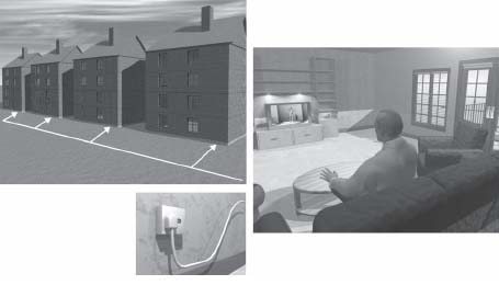
Cable TV networks get most of their channels from satellite. But some channels originate from terrestrial transmitters and other local sources.
THE HEADEND: THE HEART OF THE CABLE TV NETWORK
The basic idea of establishing cable television is that the viewer can receive a number of TV channels without any other equipment beyond his existing TV set. Therefore analog TV will live on for a long time in the cable TV networks.
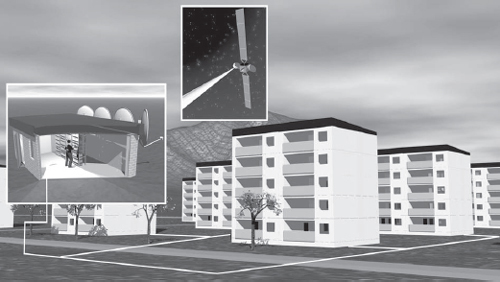
The heart of a cable TV network is the headend, a central utility where all reception is arranged. In the headend, there are a number of satellite-receiving antennas usually a bit larger than is used for individual reception. Another important difference in relation to reception in an individual home using a satellite DTH (direct to home) dish is that the antennas must be able to simultaneously receive both polarizations and both parts of the satellite downlink frequency band. In most individual home satellite receiving systems, you can only receive one channel at a time.
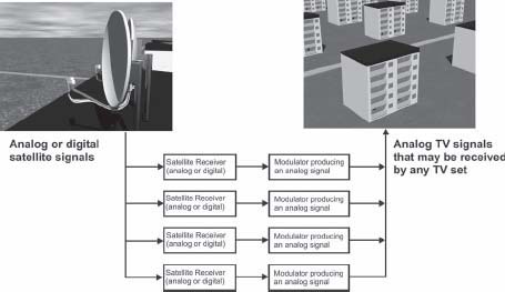
The signals from the parabolic dishes are split up in racks filled with satellite receivers. From the satellite receivers, analog audio and video signals are obtained. These signals are fed to modulators that are comparable with small TV transmitters generating analog TV channels at the desired channels numbers. This converts the digital satellite signals into analog channels, making it possible for the viewer to keep his old analog equipment.
The modulators are connected together to produce the complete package of channels that is fed into the cable TV network. Any encrypted channels will be re-encrypted before they are distributed on the network. The viewers need to have separate decoders to watch the encrypted programming.
In the beginning of the development of cable TV, there was at least one headend in each city. The reception equipment was pretty expensive in the early days of satellite TV since large dishes and expensive satellite receivers were needed. To spread the signals within the city, a large coaxial network was constructed, using existing culverts or buried in tubes. However, the cabling could end up kilometers or miles in length, so amplifiers had to be introduced at certain distances to keep the signal at usable levels.
FIGURE
5.3
The basic principle of analog cable television is to receive satellite signals and modulate them into standard terrestrial analog signals that can be received by any TV set.
The early goal of analog cable TV was to connect as many old MATV (Master Antenna TV) systems as possible to the large network that covered the whole city. This was to get as many viewers (customers) as possible. You can say that the cable TV network may be regarded as being divided into three distribution levels. In this book, I refer to them as D1, D2 and D3 levels. D1 is the top level of the network, with cabling to different areas of the city. The D2 level is the level inside the D1 area and the D3 level is the cabling inside the individual building. By the end of the 1980s, receiving equipment started to get cheaper and smaller dishes became possible for satellite reception. Cable TV began to become economical to start up at smaller locations. Even in separate buildings, satellite signals could be introduced into the local net. The large city networks started to get competition from the smaller cabling companies when satellite channels were introduced directly at the D3 level.

FIGURE
5.4
Cable TV networks may be divided into three basic distribution levels, D1, D2 and D3.
CHANNEL CAPACITY
Still, it did not prove easy to construct cable TV networks that included many TV channels. Figure 5.5 shows the frequency ranges used for European cable TV.
FIGURE
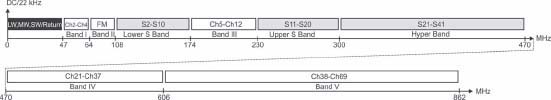
5.5
Frequency bands and channels used for cable TV in most parts of Europe.
The more bandwidth that can be used in the cables, the more channels can be distributed. In terrestrial TV, the UHF band of 470 to 862 MHz may be used. However, at these comparatively high frequencies, the signal attenuation in the cables is quite high. For this reason, early cable TV distribution was restricted to frequencies below 300 MHz. In old MATV systems, the UHF channels were down-converted to lower frequencies before being sent into the network.
Below 300 MHz, not that many channels can be used for distribution. The bandwidth of the channels are 7 MHz wide and in the lowest frequency band, band I (47–64 MHz), there are only three channels: channel 2, 3 and 4. Channel 1 does not even exist. The next frequency band, band II (87–108 MHz) is used for FM radio. The third band, band III, (174–230 MHz) covers the channels 5 through 12. Channel numbers mentioned here applies to continental Europe.
In early cable TV, only every other channel could be used because of filtering problems in older TV sets. This was not so good. The only channels available were channels 3 (band I), 5, 7 9 and 11 (band III) or channels 2, 4 (band I) and 6, 8, 10 and 12 (band III)—not a lot of options. In addition to this, some frequencies could not be used since they were already in use by terrestrial transmitters and would be exposed to interference if used. In some countries, channel 12 was not allowed to be used due to frequency coordination with other kinds of services. Today channel 12 is used for DAB (Digital Audio Broadcasting) in Europe.
To solve the bandwidth problems, two new frequency bands—the S-Bands—that were only allowed to be used in cable networks were introduced. The lower S-Band (108–174 MHz) contains the channels S2 through S10 and the upper S-Band (230–300 MHz) contains the channels S11 through S20.
For quite some time, the larger cable TV networks were restricted to the frequency range below 300 MHz. But as the amplifier technique developed, it became possible to exchange the amplifier for new one that could cover frequencies up to 400 or 500 MHz. The area between 300 and 470 MHz is the hyper band containing the channels S21 to S41 (in most countries only the channels between S21 and S38 are used.) And in this frequency range the channels have the same bandwidth as UHF channels, 8 MHz.
Initially, viewers had to use separate boxes that made it possible to receive the new frequency ranges of the S channels. But after some years, most new TV sets had built in S-channel tuners, even called cable TV tuners. Cable TV became multi-channel and the subscribers could easily receive up to 30 channels.
THE MATV (MASTER ANTENNA TV) NETWORK
In many European countries, cable TV was based on the fact that there were lots of MATV systems that easily could be hooked up the larger cable TV networks. However the quality of MATV networks varies. Most of these networks are cascaded networks (see Figure 5.6). In order to save some cabling, one cable can go from one apartment to the next passing through several outlets. But saving cable comes at a price. The signal level will get lower as the signal pass from one outlet to the next. If you are at the end outlet, your signal might be a lot worse than at the first outlet.
The alternative to the cascaded network is the star-shaped network. Each apartment has its own cable direct from the divider and each unit's signal level is not affected by other outlets. Another advantage is that there is an alternative to encryption of pay TV channels. Instead, the pay-TV content can be filtered so that only people paying would get those channels distributed on their cable.
In the beginning of cable TV, there were some high ambitions about using only star-shaped networks to benefit from these advantages. Economical realities, however, showed that this was not possible. The antenna outlets had to be exchanged and new amplifiers had to replace the old ones. However in many cases old cables were used. And in many cases there was not room for any new cables necessary to get a star-shaped structure in the old tubes and conduits. It was much easier to renovate the old cascaded networks that already existed.
FIGURE
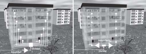
5.6
Cable TV networks with several branches, in this case in star-shaped (left) and cascaded structures (right).
The coaxial cable network within a building may be small or large. There might be a large number of branches each connected to a number of outlets. However there is a large problem. Since the signal has to be split between a numbers of outlets and may be transported in long cables, amplifiers are needed.
In Chapter 4, I mentioned that it is necessary to have only one carrier if an amplifier is to operate in saturated mode and provide maximum amplification. Unfortunately, in cable TV, there are many channels which mean that the amplifiers have to be backed off—i.e., we can only use a portion of the available amplification. The amplifiers have to work in linear mode and if they get into nonlinear mode, it will result in intermodulation and mixing of the channels. If you wish to increase the number of channels the amount of power that can be allocated to each channel will get less (see Figure 5.7).
FIGURE
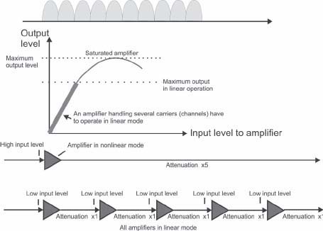
5.7
Amplifiers must operate in linear mode.
This would mean less amplification on each channel, but since a certain amount of amplification is needed on each channel to get the signal to the end outlet of the branch, the number of amplifiers also has to increase as the number of channels increase. By adding more amplifiers and reducing the input level on each amplifier, they continue to function in linear mode and the quality of the signals in the network is maintained.
UHF COAXIAL NETWORKS
Most cable TV networks are limited to the frequency area below 400 or 500 MHz. From a technical point of view, it is possible to design UHF coaxial networks handling frequencies within the 470-862 MHz range. One way of doing this is split-band techniques where the VHF and UHF frequency bands are treated separately. The UHF part of the amplifiers has higher amplification than the VHF parts since the attenuation in the cables increase with increased frequency.
COAXIAL CABLE TV NETWORKS
The MATV systems were the original cable networks. When large-scale cable television was introduced, many of these MATV systems could be reused and integrated in these larger systems. But sometimes the cables were too bad; they had a high attenuation and were too poorly insulated. This meant it was not possible to introduce S channels and avoid interfering with other services that existed in the air. However, the channels in the buildings containing the old cables could be reused for new ones. The old cables could also be used to drag the new cables along the same path in the building. In the 1980s, a lot of work was put into modernization of old MATV networks as they became a part of larger cable TV networks and got more channels. Also at this time, large cable networks covering complete cities were constructed. These networks would integrate all MATV systems into one single system that could be fed from one common headend.
When cable TV was introduced, coaxial cables were used at the D1 level, with amplifiers at suitable distances to compensate for the attenuation in the longest cables even kilometers or miles in length. The major problem is that it is not possible to distribute signals at frequencies above 500 MHz for long distances using coaxial cables (see Figure 5.8). The cable TV operators were forced to upgrade the amplifiers for higher frequency ranges as the technology in the amplifiers developed. A second problem is getting return traffic back from the viewers.
Coaxial Cable Return Traffic
If the cable TV network is to be used to provide broadband connections to the Internet, a return path from the subscriber to the network is required. An Internet connection in a cable TV network is based on using a radio receiver and transmitter for data signals. The cable modems transmit information back to the headend using frequencies below 47 MHz. In some cases, frequencies up to 64 MHz are used for return traffic.
With a lot of subscribers, the return path will get crowded. And if several heavy populated areas are connected, the situation will grow even worse.
Since there is a cable connection to every apartment, traffic in two directions would be desirable. As an example, Internet access can be provided through the cable if the return traffic is handled properly. A large wish among the cable operators was to develop something that would provide two-way communications with unlimited bandwidth at the D1 level in the networks and not have to further exchange amplifiers as development preceded. The solution was to change the coaxial cables to optical fibers.
FIGURE
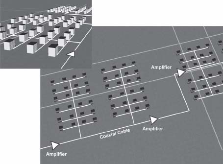
5.8
Old city cable TV networks were based on coaxial cables with amplifiers placed at suitable distances.
HYBRID FIBER COAXIAL NETWORKS (HFC)
Some years ago many people thought that it would be possible to get optical fiber into each household. This is called “fiber to the home.” This would provide an electronic highway with unlimited bandwidth into the home. However, the economical reality had proved that fiber to the home is more of a dream than reality. At least until recent developments.
The last part of the cable TV network, the cabling within the building, is the most expensive part to upgrade to fiber. In addition, the coaxial cables already exist and it is very hard to motivate an exchange. There are also practical problems in connecting the fiber to the equipment in the home. Sooner or later you have to convert to an electrical interface before connecting all devices that need to communicate with the outside. Also optical fibers are fed by lasers and may be dangerous to look into if you disconnect them yourself because this kind of laser is often not visible but still dangerous to the eyes.
Optical fibers used to connect digital audio in a home cinema between the DVD recorder and the home cinema amplifiers are not of this kind. They use ordinary LEDs (light emitting diodes) that are completely harmless. The disadvantage is that these kind of light sources only work in short lengths of fibers. Lasers are needed to reduce the attenuation of the light signal in the long fibers that would have been required for fiber to the home distribution.
There are no fibers to the home, but for professional use in the D1 level in the cable networks they have become very popular.
How Fiber Networks Work
As soon as the complete content of the cable TV network has been generated as an electrical signal, the signals are converted into laser light. Instead of distributing the electrical signal, as was done before, the signal is converted into a laser light signal by a laser diode. The laser light is fed into an optical fiber. Light is, in reality, the same physical phenomenon as radio waves. They are both electromagnetic waves, but light is at much higher frequencies. However, light is usually not characterized in frequencies but in wavelengths. One usual wavelength used in optical fibers is 1,310 nm (nanometers). In the terms that are used for radio, this would correspond to a frequency of 229,000 GHz. At these incredibly high frequencies, there is such an immense amount of bandwidth that it is hard for an ordinary human being to understand. The complete content of the cable TV network can easily be converted into a light signal using a laser. At the other end of the fiber, the light signal will hit a photo diode. The photo diode then regenerates the electrical signal.
A fiber of this kind can be kilometers or miles in length without any amplifiers between the laser and the photo diode at the other end.
When the fiber reaches a block of houses, the signal is converted into an electrical signal that is fed into the local coaxial network on the D2 level or directly into the network within a certain building on the D3 level. The lower levels of the cable network can still be used as before distributing the electrical signals.
However the main advantage in using fiber is the possibility to use several wavelengths in the fiber, making it possible to reuse the fiber several times. In the forward direction, as we have already seen, one wavelength is sufficient for all contents.
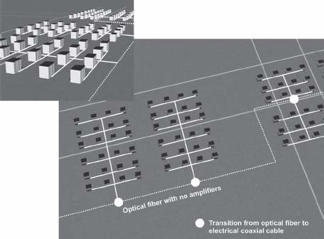
FIGURE
5.9
HFC (Hybrid Fiber Coaxial) network.
HFC Network Return Traffic
One way of solving the return path capacity problem is to collect all the radio signals from all modems within a certain area and convert them into a common optical signal.
From the different areas in the city, different wavelengths are used to carry the return traffic back to the headend. In Figure 5.10, you see four different areas that use the wavelengths 1510, 1530, 1550 and 1570 nm respectively. This way, every area within the city gets its own wavelength and the traffic within the coaxial networks in different areas does not compete with each other. Competition for return capacity within the radio spectrum of the coaxial network is limited to internal competition within that area of the network. If coaxial cable had been used at the higher level of the network, all return traffic for the complete city would have had to fight for the same capacity.
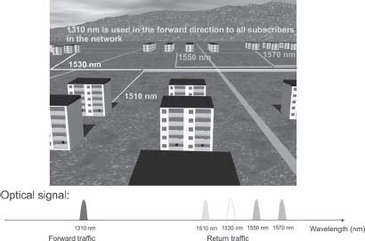
FIGURE
5.10
This HFC network uses different wavelengths for return traffic from different areas in the network. (See color plate.)
Larger cable TV operators often want to connect networks in different cities to one giant network covering a whole country. This may be done using optical fibers. However it is not possible to use the earlier described analog optical signals to do this. Instead, the content has to be digitized before being sent between the cities. Then it is converted into analog optical signals as it arrives to the next city and the end distribution takes place as described above.
DIGITAL CABLE TELEVISION
Until now, we have only discussed distribution of analog signals to the end user in the cable TV network. But of course there are also enormous possibilities to distribute digital TV in the existing cable TV networks.
The major problem related to analog cable TV is that the quality you obtain in your TV set is dependant on where in the branch of your local coaxial network your apartment or house happens to be located. In addition, cable TV subscribers buy DVD recorders and wide screen TV sets and complete home cinema systems. For this reason, there is also a demand for modern digital signals from the cable TV network.
Digital cable TV in Europe is based on the same standard, digital video broadcasting, DVB, as is used for satellite broadcasting. The nucleus of DVB is the transport stream, including the data packets that contain the audio and video information. The main difference between digital cable TV and satellite distribution is the higher level of modulation. The most common kind of modulation is 64 QAM that is a combination of amplitude and phase modulation. There are even higher levels of standardized modulation, such as 128 and 256 QAM that can be used for cable TV. However, these higher modulation schemes would demand higher quality of the signals in the cable TV networks.
Figure 5.11 shows the modulation scheme for 64 QAM. It is not easy to draw a signal, so it is symbolized by its constellation diagram showing the amplitudes and phase angles representing the symbols for each combination of bits.
64 QAM resembles QPSK but has more phase angles. Instead of four possible phase angles there are 52. And on top of this, there are 10 different amplitude levels instead of one as in QPSK. In total, there are 64 different combinations of phase angles and amplitudes that are allowed, to some extent resembling a chessboard. Each symbol then represents a combination of six bits. In other words, six bits may be transmitted simultaneously. Of course, a signal based on 64 QAM is much more sensitive to noise and disturbances than QPSK, since the symbols are located much closer to each other. Despite this, 64 QAM has a large advantage over QPSK because it is possible to get a 38 Mbit/s signal into an 8 MHz channel. 8 MHz channels are used in the hyper band and in the UHF bands. 38 Mbit/s is the same bitrate as the bitrate housed in a satellite multiplex—the content of a satellite transponder.
Setting up a complete installation, including the creation of a complete DVB signal package with MPEG 2 encoders and multiplexing of the signals, is expensive. Adding pay TV encryption services is even more costly. These investments are generally limited to large cable TV operators, which spread the costs out to hundreds of thousands of subscribers. A much less expensive way to solve this is by using the satellite multiplexes. However the satellite signals are QPSK modulated, so the signals have to be demodulated to get hold of the transport stream. The transport stream, however, can be modulated again using 64 QAM. Direct transmodulation from QPSK to 64 QAM is cheap but requires that the signal in the cable TV network can be identical to the satellite signal.
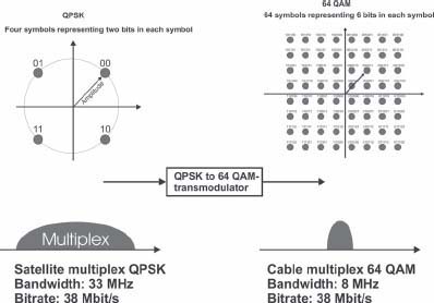
FIGURE
5.11
Transmodulation from QPSK to 64 QAM.
A problem of using the same signals in the cable TV networks as on satellite is that pay TV satellite signals are encrypted by the satellite content provider. As a result, the satellite content provider can reach customers in the cable networks. Of course this is not acceptable to the cable TV companies. In order to get the cable TV operators to keep their own encryption systems and program cards, there are different ways of modifying the transport stream before it is modulated to 64 QAM. The costs increase in relation to how much of the transport stream is to be modified. However, these kinds of modifications to maintain the structure of the original transport stream are what make it possible to distribute digital TV even in smaller cable TV networks.
Digital Cable TV Receivers
The difference between digital receivers for cable and digital satellite receivers is the input stage, which covers the input frequency ranges of cable TV. This may include frequencies up to 862 MHz since there might be cable TV operators also interested in using UHF. Also, the cable receiver has a QAM demodulator where the satellite box has a QPSK demodulator.
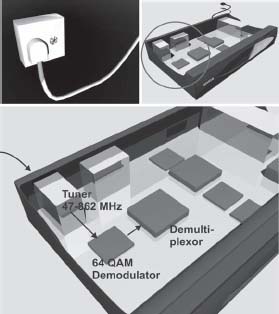
FIGURE
5.12
The digital TV receiver for cable has an input stage covering the frequency ranges for cable and uses a QAM demodulator instead of a QPSK modulator prior to the demultiplexor.
Digital cable television makes it possible to get the same content as in a complete satellite transponder into an 8 MHz channel that previously only distributed one analog channel. Today 8 to 10 TV channels in standard resolution may be housed within such a distribution channel. In addition to this, a noiseless picture is achieved in combination with improved audio. The only audio that used to be better is the NICAM stereo sound used in some of the European countries. Most cable TV operators in these countries did never introduce NICAM stereo in the cable networks, except for channels directly fed from terrestrial transmitters into the program content. Otherwise, NICAM encoding in cable networks was quite expensive.
Analog cable TV has become quite old and out of fashion but all this can be easily managed by introducing DVB signals. By using DVB, it is now also possible to introduce multi-channel AC3 audio (Dolby Digital) in the cable networks. In this way, cable TV subscribers get access to the quality and possibilities that previously only have been possible using direct satellite reception.
SMATV, SATELLITE MATV SYSTEMS
In parallel to traditional cable TV there is another kind of satellite MATV systems, the satellite i.f. (intermediate frequency) systems. In these systems, the signal from one or more satellite dish is distributed directly to a satellite receiver placed in each apartment or house. Everyone uses the same kind of satellite receiver as they would if they had a dish of their own. The only common parts are the satellite dishes and a multi-switch system. A drawback is that the households have to be located quite close to each other since distribution takes place in the frequency range of 950 to 2,150 MHz. The advantage is that each household can get the same number of channels as if they had their own dish.
However, this access comes at a price. The coaxial cable in building must be a star-shaped network with one cable to each household from the divider, and the cables have to be of the low-attenuating type. In addition, there has to be a multi-switch device that makes it possible for each viewer to select the correct LNB, polarization and part of the satellite frequency band (10.70–11.70 GHz or 11.70–12.75 GHz) to be able to watch a certain channel. Signaling to the multi-switch device may be used on the 22 kHz tone, the change of supply voltage at the LNB input of the satellite receiver or pure DiSEqC signaling. We will take a deeper look at this technology in Chapter 9, “How to Connect the Devices.” The technique described here may be regarded as a kind of MATV based on satellite instead of terrestrial reception.
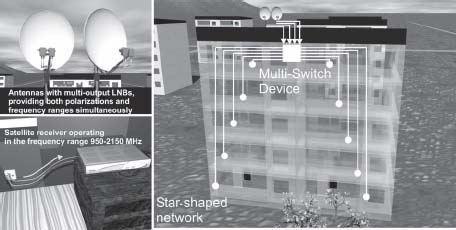
FIGURE
5.13
Using satellite i.f. distribution, every household has its own digital satellite receiver and may receive as many channels as if they had their own satellite dish. This may be regarded as a satellite MATV system.
TERRESTRIAL DIGITAL TV SIGNALS IN COAXIAL CABLE SYSTEMS
There is yet another way to supply a coaxial cable network with digital TV signals. Every household can have a terrestrial digital receiver but share the same antenna system. The drawback (compared to 64 QAM based digital cable television) is that a terrestrial TV channel according to the European DVB-T standard and that is 8 MHz wide only can handle a bitrate of about 22 Mbit/s compared to 38 Mbit/s using 64 QAM. The advantage (compared to the satellite i.f. distribution system) is that ordinary cable TV networks operating at frequencies in the VHF and UHF frequency bands may be used. It is also possible to distribute the signals in networks having cascaded outlets.
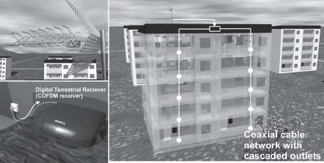
FIGURE
5.14
A third way of supplying a coaxial cable network with digital TV is using signals from terrestrial digital TV transmitters. This technique resembles traditional MATV but in a digital shape.
The terrestrial TV signals will be discussed more in detail in Chapter 6, “Digital TV by Terrestrial Transmitters.”
The strength of cable TV is that it is possible to let several households share the same signal source. This is ideal for people who do not wish to worry about the reception equipment themselves. The drawback is that programming choices may be limited, relative to having a reception system completely on your own. You have to rely on the signals the cable operator has put into the network and what technology is used for the distribution.