26
Why Tactical Macro Investing Still Makes Sense
Jason Gerlach, Rick Slaughter, Chris Stanton
Sunrise Capital Partners
Introduction
In November 2002, Cass Business School Professor Harry M. Kat, Ph.D. began to circulate a working paper entitled “Managed Futures and Hedge Funds: A Match Made in Heaven.” The Journal of Investment Management subsequently published the paper in the First Quarter of 2004. We consider Dr. Kat’s paper to be one of the seminal works in the tactical macro investing or “managed futures” space. In the paper, Kat noted that while adding hedge fund exposure to traditional portfolios of stocks and bonds increased returns and reduced volatility, it also produced an undesirable side effect—increased tail risk (lower skew and higher kurtosis). He went on to analyze the effect of adding managed futures to the traditional portfolios, and then of combining hedge funds and managed futures, and finally the effect of adding both hedge funds and managed futures to the traditional portfolios. He found that managed futures were better diversifiers than hedge funds, that managed futures reduced the portfolio’s volatility to a greater degree and more quickly than did hedge funds, and that managed futures achieved this without the negative side effect of increased tail risk. He concluded that the most desirable results were obtained by combining both managed futures and hedge funds with the traditional portfolios.1
Kat’s original period of study was June 1994–May 2001. In our paper, we revisit and update Kat’s original work. Hence, our primary period of study is the “out-of-sample” period since then, which is January 2001–December 2015. In two appendices, we also include our findings for two other periods. Due to the availability of the data and our choice of it, in Appendix A, we share our results for the entire period from 1990–2015.
This encompasses the almost four and a half years prior to Kat’s original study period, Kat’s original study period, and the out-of-sample period since then. In Appendix B, we share our results for the exact same period that Kat studied in his paper (June 1994–May 2001). It is important to note that our paper in general and Appendix B specifically is not meant to be an exact replication of Kat’s original work.
Managed Futures
Managed futures may be thought of as a collection of liquid, transparent, tactical macro hedge fund strategies which focus on exchange-traded futures, forwards, options, and foreign exchange markets. Trading programs take both long and short positions in as many as 400 globally diversified markets, spanning physical commodities, fixed income, equity indices, and currencies. Daily participants in these markets include hedgers, traders, and investors, many of whom make frequent adjustments to their positions, contributing to substantial trading volume and plentiful liquidity. These conditions allow most managed futures programs to accommodate large capacity and provide the opportunity to diversify across many different markets, sectors, and time horizons.2
Diversification across market sectors, active management, and the ability to take long and short positions are key features that differentiate managed futures strategies not only from passive, long-only commodity indices, but from traditional investing as well.3 Although most managed futures programs trade equity index, fixed income, and foreign exchange futures, their returns have historically been uncorrelated to the returns of these asset classes.3 The reason for this is that most managers are not simply taking on systematic beta exposure to an asset class, but are attempting to add alpha through active, tactical management and the freedom to enter short or spread positions, tactics which offer the potential for completely different return profiles than long-only, passive indices.3
Early stories of futures trading can be traced as far back as the late 1600s in Japan.4 Although the first public futures fund started trading in 1948, the industry did not gain traction until the 1970s. According to Barclays (2012), “a decade or more ago, these managers and their products may have been considered different than hedge funds; they are now usually viewed as a distinct strategy or group of strategies within the broader hedge fund universe. In fact, managed futures represent an important part of the alternative investment landscape,” commanding approximately 12% of all hedge fund assets, which equated to $333.4 billion at the end of Q3 of 2015.5
Managed futures can be thought of as a subset of global macro strategies that focuses on global futures and foreign exchange markets and is likely to utilize a highly tactical, systematic approach to trading and risk management. The instruments that are traded tend to be exchange-listed futures or extremely deep, liquid, cash-forward markets. Futures facilitate pricing and valuation and minimize credit risk through daily settlement, enabling hedge fund investors to mitigate or eliminate some of the more deleterious risks associated with investing in alternatives. Liquidity and ease of pricing also assist risk management by making risks easier to measure and model.3 In research conducted before the Global Financial Crisis, Bhaduri and Art (2008) found that the value of liquidity is often underestimated, and, as a result, hedge funds that trade illiquid instruments have underperformed hedge funds that have better liquidity terms.6
The quantitative nature of many managed futures strategies makes it easy for casual observers to mistakenly categorize them as “black box” trading systems.3 According to Ramsey and Kins (2004), “The irony is that most CTAs will provide uncommonly high levels of transparency relative to other alternative investment strategies.”7 They go on to suggest that CTAs are generally willing to describe their trading models and risk management in substantial detail during the course of due diligence, “short of revealing their actual algorithms.” CTAs are also typically willing to share substantial position transparency with fund investors. Through managed accounts, investors achieve real-time, full transparency of positions and avoid certain custodial risks associated with fund investments. Ramsey and Kins conclude that, “It is difficult to call CTAs black box, considering they disclose their methodology and provide full position transparency so that investors can verify adherence to that methodology.”
Separately managed accounts, common among managed futures investors, greatly enhance risk management by providing the investor with full transparency, and in extreme cases, the ability to intervene by liquidating or neutralizing positions.3 In addition, institutional investors who access CTAs via separately managed accounts substantially reduce operational risks and the possibility of fraud by maintaining custody of assets. Unlike the products traded in other hedge fund strategies, those traded by CTAs allow investors to customize the allocation by targeting a specific level of risk through the use of notional funding. The cash efficiency made possible by the low margin requirements of futures and foreign exchange allows investors to work with the trading manager to lever or delever a managed account to target a specific level of annualized volatility or other risk metric. Some CTAs offer funds with share classes with different levels of risk. Unlike traditional forms of leverage, which require the investor to pay interest to gain the additional exposure, assets used for margin in futures accounts can earn interest for the investor.
Another advantage of trading futures is that there are no barriers to short selling. Two parties simply enter into a contract; there is no uptick rule, there is no need to borrow shares, pay dividends, or incur other costs associated with entering into equity short sales. Thus, it is easier to implement a long-short strategy via futures than it is using equities.3
Defining Managed Futures and CTAs
“Managed futures” is an extremely broad term that requires a more specific definition. Managed futures traders are commonly referred to as “Commodity Trading Advisors” or “CTAs,” a designation which refers to a manager’s registration status with the Commodity Futures Trading Commission and National Futures Association. CTAs may trade financial and foreign exchange futures, so the Commodity Trading Advisor registration is somewhat misleading since CTAs are not restricted to trading only commodity futures.3
Where Institutional Investors Position Managed Futures and CTAs
According to a survey in the Barclays February 2012 Hedge Fund Pulse report, institutional investors view the top three key benefits of investing in CTAs as:
- Low correlation to traditional return sources
- The risk-mitigation/portfolio-diversifying characteristics of the strategy
- The absolute-return component of the strategy and its attributes as a source of alpha
Also, 50% of the investors surveyed have between 0% to 10% of their current hedge fund portfolio allocated to CTA strategies, and 50% of investors surveyed plan to increase their allocations to the strategy in the next six months.5
Skewness and Kurtosis
When building portfolios using the Modern Portfolio Theory (MPT) framework, investors focus almost solely on the first two moments of the distribution: mean and variance. The typical MPT method of building portfolios appears to work well, as long as historical correlations between asset classes remain stable.8 But in times of crisis, asset classes often move in lock-step, and investors who thought they were diversified experience severe “tail-risk” events. By only focusing on mean return and variance, investors may not be factoring in important, measurable, and historically robust information.
Skewness and kurtosis, the third and fourth moments of the distribution, can offer vital information about the real-world return characteristics of asset classes and investment strategies. The concepts of skewness and kurtosis are paramount to this study.
- Skewness is a measure of symmetry and compares the length of the two “tails” of a distribution curve.
- Kurtosis is a measure of the peakedness of a distribution—i.e., do the outcomes produce a “tall and skinny” or “short and squat” curve? In other words, is the volatility risk located in the tails of the distribution or clustered in the middle?
To understand how vital these concepts are to the results of this study, we revisit Kat’s original work. Kat states that when past returns are extrapolated, and risk is defined as standard deviation, hedge funds do indeed provide investors with the best of both worlds: an expected return similar to equities, but risk similar to that of bonds. However, Amin and Kat (2003) showed that including hedge funds in a traditional investment portfolio may significantly improve the portfolio’s mean-variance characteristics, but during crisis periods, hedge funds can also be expected to produce a more negatively skewed distribution.9 Kat (2004) adds, “The additional negative skewness that arises when hedge funds are introduced [to] a portfolio of stocks and bonds forms a major risk, as one large negative return can destroy years of careful compounding.”1
Kat’s finding appears to be substantiated in Koulajian and Czkwianianc (2011), which evaluates the risk of disproportionate losses relative to volatility in various hedge fund strategies10:
“Negatively skewed strategies are only attractive during stable market conditions. During market shocks (e.g., the three largest S&P 500 drawdowns in the past 17 years), low-skew strategies display:
- Outsized losses of –41% (vs. gains of +39% for high-skew strategies);
- Increases in correlation to the S&P 500; and
- Increases in correlation to each other”
Skewness and kurtosis may convey critical information about portfolio risk and return characteristics, something that should be kept in mind when reading this study. [A more thorough review of skewness and kurtosis can be found in Appendix C.]
Data
Like Kat, our analysis focuses upon four asset classes: stocks, bonds, hedge funds, and managed futures.
- Stocks—represented by the S&P 500 Total Return Index. The S&P 500 has been widely regarded as the most representative gauge of the large cap U.S. equities market since the index was first published in 1957. The index has over US$7.8 trillion benchmarked against it, with index-replication strategies comprising approximately US$2.2 trillion of this total. The index includes 500 leading companies in leading industries of the U.S. economy, capturing 80% of the capitalization of equities. The S&P 500 Total Return Index reflects both changes in the prices of stocks as well as the reinvestment of the dividend income from the underlying constituents.
- Bonds—represented by the Barclays U.S. Aggregate Bond Index (formerly the Lehman Aggregate Bond Index). It was created in 1986, with backdated history to 1976. The index is the dominant index for U.S. bond investors, and is a benchmark index for many U.S. index funds. The index is a composite of four major sub-indexes: the U.S. Government Index; the U.S. Credit Index; the U.S. Mortgage-Backed Securities Index (1986); and (beginning in 1992) the U.S. Asset-Backed Securities Index. The index tracks investment-quality bonds based on S&P, Moody, and Fitch bond ratings. The index does not include High-Yield Bonds, Municipal Bonds, Inflation-Indexed Treasury Bonds, or Foreign Currency Bonds. As of late 2015, the index is comprised of about 8,200 bond issues.
- Hedge Funds—represented by the HFRI Fund Weighted Composite Index, which includes over 2,300 constituent hedge funds. It is an equal-weighted index that includes both domestic and offshore funds—but no funds of funds. All funds report in USD and report net of all fees on a monthly basis. The funds must have at least $50 million under management or have been actively trading for at least 12 months.
- Managed Futures—represented by the Barclay Systematic Traders Index. This index is an equal-weighted composite of managed programs whose approach is at least 95% systematic.
Closing 2015, there are 454 systematic programs included in the index.
Basic Statistics
The basic performance statistics for our four asset classes are shown in Table 26.1. Similar to Kat’s results, but to a much lesser extent, our results show that managed futures have a lower mean return than hedge funds. Managed futures also have a higher standard deviation. However, they exhibit positive instead of negative skewness and much lower kurtosis. This is a critical point: the lower kurtosis conveys that less of the standard deviation is coming from the tails (lower tail risk), and the positive skewness indicates a tendency for upside surprises, not downside. From the correlation matrix, we see that hedge funds are highly correlated to stocks (0.80), managed futures are somewhat negatively correlated to stocks (–0.17), and the correlation between managed futures and hedge funds is low (0.07).
TABLE 26.1 Monthly Statistics for Stocks, Bonds, Hedge Funds, and Managed Futures for the Period June 2011–December 2015
| Stocks | Bonds | Hedge Funds | Managed Futures | |
| Mean (%) | 0.50 | 0.42 | 0.45 | 0.33 |
| Standard Deviation (%) | 4.32 | 1.01 | 1.72 | 2.25 |
| Skewness | –0.63 | –0.33 | –0.84 | 0.22 |
| Excess Kurtosis | 1.17 | 1.37 | 2.06 | 0.43 |
| Correlations | ||||
| Stocks | 1.00 | |||
| Bonds | –0.11 | 1.00 | ||
| Hedge Funds | 0.80 | –0.03 | 1.00 | |
| Managed Futures | –0.17 | 0.24 | 0.07 | 1.00 |
Stocks, Bonds, Plus Hedge Funds or Managed Futures
In order to study the effect of allocating to hedge funds and managed futures, we form a baseline “traditional” portfolio that is 50% stocks and 50% bonds (“50/50”). We then begin adding hedge funds or managed futures in 5%-allocation increments. As in Kat’s original paper, when adding in hedge funds or managed futures, the original 50/50 portfolio will reduce its stock and bond holdings proportionally. This produces portfolios such as 40% stocks, 40% bonds, and 20% hedge funds, or 35% stocks, 35% bonds, and 30% managed futures. (Note: All portfolios throughout the paper are rebalanced monthly.) Similar to Kat, we studied the differences in how hedge funds and managed futures combine with stocks and bonds. Kat found that during the period he studied, adding hedge funds to the 50/50 portfolio of stocks and bonds lowered the standard deviation, as hoped for. Unfortunately, hedge funds also increased the negative tilt of the distribution. In addition to the portfolios becoming more negatively skewed, the return distribution’s kurtosis increased, indicating “fatter tails.” However, Kat found that when he increased the managed futures allocation, the standard deviation dropped faster than with hedge funds, the kurtosis was lowered, and, most impressively, the skewness actually shifted in a positive direction (see Table 26.2). Kat (2004) summarized by saying, “Although [under the assumptions made] hedge funds offer a somewhat higher-than-expected return, from an overall risk perspective, managed futures appear to be better diversifiers than hedge funds.”1
TABLE 26.2 Monthly Return Statistics for 50/50 Portfolios of Stocks, Bonds, and Hedge Funds or Managed Futures for the Period January 2001–December 2015
| HEDGE FUNDS | MANAGED FUTURES | ||||||||
| HF (%) | Mean (%) | StDev (%) | Hedge Funds | Kurtosis | HF (%) | Mean (%) | StDev (%) | Hedge Funds | Kurtosis |
| 0 | 0.46 | 2.17 | Skew | 2.27 | 0 | 0.46 | 2.17 | Skew | 2.27 |
| 5 | 0.46 | 2.13 | –0.80 | 2.28 | 5 | 0.45 | 2.05 | –0.74 | 2.05 |
| 10 | 0.46 | 2.09 | –0.81 | 2.3 | 10 | 0.45 | 1.94 | –0.69 | 1.79 |
| 15 | 0.46 | 2.05 | –0.82 | 2.31 | 15 | 0.44 | 1.83 | –0.63 | 1.49 |
| 20 | 0.46 | 2.02 | –0.84 | 2.32 | 20 | 0.43 | 1.74 | –0.55 | 1.16 |
| 25 | 0.46 | 1.98 | –0.85 | 2.33 | 25 | 0.43 | 1.66 | –0.45 | 0.82 |
| 30 | 0.46 | 1.95 | –0.86 | 2.34 | 30 | 0.42 | 1.59 | –0.35 | 0.49 |
| 35 | 0.46 | 1.92 | –0.87 | 2.35 | 35 | 0.41 | 1.53 | –0.24 | 0.19 |
| 40 | 0.46 | 1.89 | –0.88 | 2.35 | 40 | 0.41 | 1.49 | –0.13 | –0.03 |
| 45 | 0.46 | 1.87 | –0.89 | 2.35 | 45 | 0.40 | 1.47 | –0.04 | –0.18 |
| 50 | 0.46 | 1.84 | –0.90 | 2.35 | 50 | 0.39 | 1.47 | 0.04 | –0.23 |
Note. HF% = hedge fund allocation percentage; StDev(%) = standard deviation.
Our results show that Kat’s observations have held up during the period since his original study. When we increased the hedge fund allocation, the portfolio return went up and the standard deviation went down. However, the previously discussed “negative side effect” of adding hedge funds was present, as the skewness of the portfolio fell and the kurtosis went up. On the other hand, when we added managed futures into the traditional portfolio, we observed more impressive diversification characteristics. In fact, managed futures appear to have improved the performance profile even more in this period, compared to the one Kat studied. Adding managed futures exposure increased mean return and simultaneously increased the skewness of –0.78 of the traditional portfolio to –0.04 at the 45% allocation level. The standard deviation dropped more and faster than it did with hedge funds, and kurtosis also improved, dropping from 2.27 to –0.18 at the 45% allocation level.
Hedge Funds Plus Managed Futures
Table 26.3 summarizes the results of combining only hedge funds and managed futures. The mean monthly return for managed futures is lower than hedge funds, so we may expect adding them in will reduce the expected return of the portfolio. The standard deviation of managed futures is higher than hedge funds, so one might expect upward pressure on volatility from the addition of managed futures. However, this is not what happens when they are combined. Due to their positive skewness and significantly lower kurtosis, adding managed futures to hedge funds appears to provide a substantial improvement to the overall risk profile. With 40% invested in managed futures, the standard deviation drops from 1.72% to 1.42%, but the expected return only declines by 5 basis points. At the same allocation to managed futures, skewness increases from –0.84 to 0.10, while kurtosis drops noticeably from 2.06 to –0.18. Hedge funds are impressive on their own, but managed futures demonstrate that they are the ultimate teammate by improving the return characteristics of the overall portfolio.
TABLE 26.3 Monthly Return Statistics for Portfolios of Hedge Funds and Managed Futures for the Period January 2001–December 2015
| MF(%) | Mean(%) | StDev(%) | Skew | Kurtosis |
| 0 | 0.45 | 1.72 | –0.84 | 2.06 |
| 5 | 0.45 | 1.64 | –0.73 | 1.73 |
| 10 | 0.44 | 1.58 | –0.61 | 1.37 |
| 15 | 0.43 | 1.52 | –0.48 | 1.00 |
| 20 | 0.43 | 1.48 | –0.34 | 0.65 |
| 25 | 0.42 | 1.44 | –0.21 | 0.33 |
| 30 | 0.42 | 1.42 | –0.09 | 0.09 |
| 35 | 0.41 | 1.41 | 0.02 | –0.08 |
| 40 | 0.40 | 1.42 | 0.10 | –0.18 |
| 45 | 0.40 | 1.44 | 0.16 | –0.20 |
| 50 | 0.39 | 1.47 | 0.19 | –0.17 |
Note. MF% = managed fund allocation percentage; StDev(%) = standard deviation.
Stocks, Bonds, Hedge Funds, and Managed Futures
The last step in our analysis is to study the effects of combining all four asset classes in one portfolio. Like Kat, we accomplish this in two steps. First, we combine hedge funds and managed futures into what we call the “alternatives portfolio.” Next, we combine this alternative portfolio with increasing amounts of a static 50/50 stocks and bonds “traditional portfolio.” With this advanced analysis, we are trying to answer two questions simultaneously. First, “What is the best combination of traditional and alternative investments?” (see axis in Figure 26.1 labeled “% in Alternatives”) and second, “What is the best mix of hedge funds and managed futures within the alternatives portfolio?” (see axis in Figure 26.2 labeled “% in Managed Futures”).

FIGURE 26.1 Mean return of varying allocation between traditional and alternative portfolios, while changing the alternative portfolio’s Managed Futures/Hedge Fund composition, for the period January 2001–December 2015

FIGURE 26.2 Standard deviation of varying allocation between traditional and alternative portfolios, while changing the alternative portfolio’s Managed Futures/Hedge Fund composition for the period January 2001–December 2015
Figure 26.1 shows that the highest mean return is obtained when the portfolio is not allocated to managed futures. Adding managed futures has a downward effect on mean return because its return is lower (0.33% vs. 0.45% for hedge funds and 0.46% for stocks and bonds). This is to be expected, as managed futures firms weigh the minimization of their standard deviation and drawdown just as heavily into their investment decisions as they do maximizing their return.
Figure 26.2 begins to tell a more intriguing story. Very similar to Kat’s results, we find that adding alternatives to traditional portfolios of stocks and bonds significantly reduces the portfolio’s standard deviation of returns. (Note: Regarding the axis labels on the figures, the author selected the viewing angle that best conveys the information in each figure. Hence, beginning with Figure 26.2, the axis labels are not necessarily consistent with those of other figures.) Moreover, this effect would have historically been optimal at a 100% allocation to alternatives with 35% of the alternatives portfolio allocated to managed futures.
Figure 26.3 shows the results of dividing returns by standard deviation, a common risk-adjusted return metric. It can be argued that the consistency of an investor’s returns is just as important as the average amount returned, or in other words, the most upside per unit of risk. We can see a maximum risk-adjusted return when invested in 100% with about 30% of that in managed futures.

FIGURE 26.3 Risk-adjusted return of 50/50 portfolios of stocks, bonds, hedge funds, and managed futures for the period of January 2001–December 2015
Figure 26.4 shows the skewness results for the combined portfolios. We find that adding exposure to alternatives exerts a desirable upward effect on skewness. In turn, as the managed futures allocation is increased, the positive effect on skewness is increased. At levels starting at approximately 80% allocation to alternatives, the skewness of the portfolios actually becomes positive. The highest levels of skewness were found at an 100% allocation to alternatives with more than half allocated to managed futures.

FIGURE 26.4 Skewness of 50/50 portfolios of stocks, bonds, hedge funds, and managed futures for the period June 2001–December 2015
Finally, Figure 26.5 shows the results as they pertain to kurtosis. Like Kat, we find that allocation of managed futures favorably decreases the portfolio’s kurtosis, and with 95%–100% allocated to alternatives and 40%–55% of the alternatives portfolio allocated to managed futures it actually produces a negative kurtosis of –0.19.
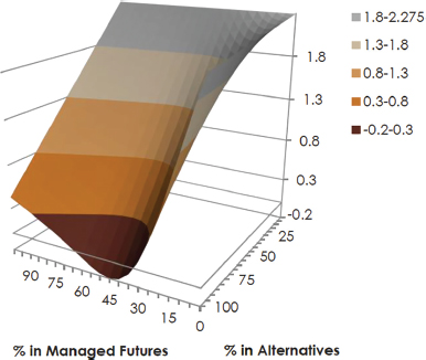
FIGURE 26.5 Kurtosis of 50/50 portfolios of stocks, bonds, hedge funds, and managed futures for the period June 2001–December 2015
We repeated the analysis above with several other CTA indices to make sure that our results were not specific to one index in particular. In all cases, the results were very similar to what we found above, suggesting that our results are robust irrespective of the choice of managed futures index.
Conclusion
In this study, we used the framework introduced by Dr. Harry M. Kat in his paper Managed Futures and Hedge Funds: A Match Made in Heaven to analyze the possible role of managed futures in portfolios of stocks, bonds, and hedge funds. Our aim with this paper was to discover whether or not Kat’s findings have held up in the years since.
Managed futures have continued to be very valuable diversifiers. Throughout our analysis, and similar to Kat, we found that adding managed futures to portfolios of stocks and bonds reduced portfolio standard deviation to a greater degree and more quickly than did hedge funds alone, and without the undesirable side effects of skewness and kurtosis.
The most impressive results were observed when combining both hedge funds and managed futures with portfolios of stocks and bonds. Figures 26.1 to 26.5 showed that the most desirable levels of mean return, standard deviation, skewness, and kurtosis were produced by portfolios with allocations of 90%–100% to alternatives and 40%–55% of the alternatives portfolio allocated to managed futures.
As a finale, we thought it would be instructive to show performance statistics for portfolios that combine all four of the asset classes: stocks, bonds, managed futures, and hedge funds. Table 26.4 shows the results for portfolios ranging from a 100% Traditional portfolio (50% stocks/50% bonds) to a 100% Alternatives portfolio (50% hedge funds/50% managed futures) in 10% increments.
TABLE 26.4 Performance Statistics for Portfolios Ranging from 100% Traditional Portfolio to 100% Alternatives Portfolio in 10% increments for the Period January 2001–December 2015
| Stocks(%) | Bonds(%) | HF(%) | MF(%) | Mean(%) | StDev(%) | Skew | Kurt | Return/Risk |
| 50 | 50 | 0 | 0 | 0.46 | 2.66 | –0.47 | 1.29 | 0.17 |
| 45 | 45 | 5 | 5 | 0.45 | 2.59 | –0.46 | 1.28 | 0.17 |
| 40 | 40 | 10 | 10 | 0.45 | 2.53 | –0.44 | 1.28 | 0.18 |
| 35 | 35 | 15 | 15 | 0.44 | 2.46 | –0.42 | 1.28 | 0.18 |
| 30 | 30 | 20 | 20 | 0.43 | 2.39 | –0.41 | 1.27 | 0.18 |
| 25 | 25 | 25 | 25 | 0.42 | 2.32 | –0.39 | 1.27 | 0.18 |
| 20 | 20 | 30 | 30 | 0.42 | 2.26 | –0.37 | 1.26 | 0.19 |
| 15 | 15 | 35 | 35 | 0.41 | 2.19 | –0.36 | 1.26 | 0.19 |
| 10 | 10 | 40 | 40 | 0.40 | 2.12 | –0.34 | 1.25 | 0.19 |
| 5 | 5 | 45 | 45 | 0.40 | 2.05 | –0.32 | 1.25 | 0.19 |
| 0 | 0 | 50 | 50 | 0.39 | 1.99 | –0.31 | 1.25 | 0.20 |
Note. Return/Risk calculated using annualized mean and standard deviation. HF(%) = hedge fund allocation percentage, MF(%) = managed futures allocation percentage, StDev(%) = standard deviation, Kurt = kurtosis.
In Table 26.4 and Figure 26.6 (an efficient frontier based on the data in Table 26.4), the benefits of allocating to alternatives with a sizable percentage allocated to managed futures are quite compelling. As the contribution to alternatives increases, all metrics benefit:

FIGURE 26.6 Efficient frontier for portfolios ranging from 100% Traditional portfolio to 100% Alternatives portfolio in 10% increments for the period June 2001–December 2015
- Risk-adjusted return increases
- Standard deviation decreases
- Skewness increases
- Kurtosis decreases
Overall, our analysis is best summarized by the following quote from Dr. Kat (regarding his own findings almost 10 years ago): “Investing in managed futures can improve the overall risk profile of a portfolio far beyond what can be achieved with hedge funds alone. Making an allocation to managed futures not only neutralizes the unwanted side effects of hedge funds, but also leads to further risk reduction. Assuming managed futures offer an acceptable expected return, all of this comes at quite a low price in terms of expected return foregone.”1
Appendix A
In this appendix, we present the results of our analysis via data tables and graphics in the same format as the main body of the study, but for the period January 1990–December 2015. The data we used in our study, particularly the hedge fund and CTA indices, allowed us to go back to 1990, almost four and a half years prior to the start of Kat’s study period. Besides analyzing the out-of-sample period since Kat’s study period, we thought analyzing the entire period from 1990–2015 would be both instructive and interesting (Table A-1).
TABLE A-1 Monthly Statistics for Stocks, Bonds, Hedge Funds, and Managed Futures for the Period January 1990–December 2015
| Stocks | Bonds | Hedge Funds | Managed Futures | |
| Mean (%) | 0.83 | 0.52 | 0.83 | 0.54 |
| Standard Deviation (%) | 4.2 | 1.05 | 1.94 | 2.86 |
| Skewness | –0.58 | –0.22 | –0.62 | 0.75 |
| Excess Kurtosis | 1.19 | 0.74 | 2.54 | 2.11 |
| Correlations | ||||
| Stocks | 1.00 | |||
| Bonds | 0.11 | 1.00 | ||
| Hedge Funds | 0.74 | 0.09 | 1.00 | |
| Managed Futures | –0.11 | 0.21 | 0.02 | 1.00 |
In Table A-2, adding managed futures to a 50/50 portfolio of stocks and bonds increased the kurtosis for this period due to a single data point. In December 1991 managed futures produced a 14.49% return for the month, which substantially increased both the skew and kurtosis for the period. This is a prime example of our contention that skewness and kurtosis are connected and should not be analyzed in isolation. The significantly higher kurtosis, in this case, is due to the significantly higher skew caused by one positive outlier (i.e., upside volatility), in December 1991.
TABLE A-2 Monthly Return Statistics for 50/50 Portfolios of Stocks, Bonds, and Hedge Funds or Managed Futures for the Period January 1990–December 2015
| HF(%) | Mean(%) | StDev(%) | Skew | Kurt | MF(%) | Mean(%) | StDev(%) | Skew | Kurt |
| 0 | 0.67 | 2.32 | 4 | 1.46 | 0 | 0.67 | 2.32 | –0.54 | 1.46 |
| 5 | 0.68 | 2.18 | –0.57 | 1.50 | 5 | 0.67 | 2.11 | –0.46 | 1.33 |
| 10 | 0.69 | 2.15 | –0.60 | 1.55 | 10 | 0.66 | 2.01 | –0.37 | 1.24 |
| 15 | 0.70 | 2.11 | –0.64 | 1.60 | 15 | 0.65 | 1.92 | –0.25 | 1.22 |
| 20 | 0.70 | 2.08 | –0.67 | 1.65 | 20 | 0.65 | 1.84 | –0.10 | 1.30 |
| 25 | 0.71 | 2.04 | –0.71 | 1.70 | 25 | 0.64 | 1.78 | 0.06 | 1.50 |
| 30 | 0.72 | 2.02 | –0.74 | 1.75 | 30 | 0.63 | 1.74 | 0.23 | 1.83 |
| 35 | 0.73 | 1.99 | –0.76 | 1.81 | 35 | 0.63 | 1.72 | 0.40 | 2.25 |
| 40 | 0.74 | 1.97 | –0.79 | 1.87 | 40 | 0.62 | 1.71 | 0.56 | 2.71 |
| 45 | 0.74 | 1.95 | –0.81 | 1.93 | 45 | 0.61 | 1.73 | 0.70 | 3.12 |
| 50 | 0.75 | 1.93 | –0.82 | 1.99 | 50 | 0.61 | 1.77 | 0.79 | 3.42 |
Note: StDev(%) = standard deviation, Kurt = kurtosis.
To help gauge the effect of that one particular data point, we recalculated the statistics for the period, intentionally omitting the December 1991 data point. In doing so we found that at the 50% allocation level to managed futures, the skewness of the portfolio decreased slightly from 0.78 to 0.5 and kurtosis dropped from 1.54 to 1.16. Said another way, without the effect of the December 1991 data point, the statistics are more in line with our other two periods of study in this paper.
TABLE A-3 Monthly Return Statistics for Portfolios of Hedge Funds and Managed Futures for the Period January 1990–December 2015
| MF(%) | Mean(%) | StDev(%) | Skew | Kurt |
| 0 | 0.83 | 1.94 | –0.62 | 2.54 |
| 5 | 0.81 | 1.85 | –0.51 | 2.14 |
| 10 | 0.80 | 1.78 | –0.38 | 1.72 |
| 15 | 0.78 | 1.71 | –0.22 | 1.32 |
| 20 | 0.77 | 1.67 | –0.05 | 0.99 |
| 25 | 0.76 | 1.63 | 0.14 | 0.79 |
| 30 | 0.74 | 1.62 | 0.32 | 0.73 |
| 35 | 0.73 | 1.63 | 0.48 | 0.82 |
| 40 | 0.71 | 1.65 | 0.61 | 1.02 |
| 45 | 0.70 | 1.69 | 0.71 | 1.28 |
| 50 | 0.68 | 1.74 | 0.78 | 1.54 |
Note: StDev(%) = standard deviation, Kurt = kurtosis.

FIGURE A-1 Mean return of 50/50 portfolios of stocks, bonds, hedge funds, and managed futures for the period January 1990–December 2015

FIGURE A-2 Standard deviation of 50/50 portfolios of stocks, bonds, hedge funds, and managed futures for the period January 1990–December 2015

FIGURE A-3 Skewness of 50/50 portfolios of stocks, bonds, hedge funds, and managed futures for the period January 1990–December 2015

FIGURE A-4 Kurtosis of 50/50 portfolios of stocks, bonds, hedge funds, and managed futures for the period January 1990–December 2015
Appendix B
In this appendix, we present the results of our analysis via data tables and graphics in the same format as the main body of the study, but for the exact same period that Kat studied in his paper (June 1994–May 2001). It is important to keep in mind that we used different data than Kat:
- To represent “bonds,” Kat used a 10-year Government Bond Index, while we used the Barclays U.S. Aggregate Bond Index (formerly the Lehman Aggregate Bond Index).
- For “hedge funds,” Kat used his own methodology to build hedge fund portfolios with data from Tremont TASS, while we used the HFRI Fund Weighted Composite Index.
- While we and Kat both used the S&P 500 Total Return Index to represent “stocks,” Kat capped its mean return at 1% per month, while we used its exact return stream.
- For “managed futures,” Kat used the Stark 300 Index and we used the Barclay Systematic Traders Index.
After factoring in all of these differences, we were pleasantly surprised at how closely our results resembled Kat’s work from over 10 years ago.
TABLE B-1 Monthly Statistics for Stocks, Bonds, Hedge Funds, and Managed Futures for Kat’s Study Period of June 1994–May 2001
| Stocks | Bonds | Hedge Funds | Managed Futures | |
| Mean (%) | 1.46 | 0.63 | 1.16 | 0.65 |
| Standard Deviation (%) | 4.39 | 1.03 | 2.36 | 2.89 |
| Skewness | –0.81 | 0.12 | –0.67 | 0.34 |
| Excess Kurtosis | 1.05 | 0.38 | 2.95 | 0.31 |
| Correlations | ||||
| Stocks | 1.00 | |||
| Bonds | 0.22 | 1.00 | ||
| Hedge Funds | 0.70 | 0.01 | 1.00 | |
| Managed Futures | –0.05 | 0.32 | –0.02 | 1.00 |
TABLE B-2 Monthly Return Statistics for 50/50 Portfolios of Stocks, Bonds, and Hedge Funds or Managed Futures for Kat’s Study Period of June 1994–May 2001
| HF(%) | Mean(%) | StDev(%) | Skew | Kurt | MF(%) | Mean(%) | StDev(%) | Skew | Kurt |
| 0 | 1.04 | 2.36 | –0.59 | 0.04 | 0 | 1.04 | 2.36 | –0.59 | 0.04 |
| 5 | 1.05 | 2.32 | –0.64 | 0.17 | 5 | 1.02 | 2.25 | –0.53 | –0.14 |
| 10 | 1.06 | 2.30 | –0.70 | 0.32 | 10 | 1.01 | 2.20 | –0.46 | –0.29 |
| 15 | 1.06 | 2.25 | –0.75 | 0.48 | 15 | 0.99 | 2.06 | –0.38 | –0.40 |
| 20 | 1.07 | 2.23 | –0.81 | 0.52 | 20 | 0.97 | 1.99 | –0.30 | –0.45 |
| 25 | 1.07 | 2.20 | –0.85 | 0.85 | 25 | 0.95 | 1.93 | –0.22 | –0.43 |
| 30 | 1.08 | 2.18 | –0.90 | 1.05 | 30 | 0.93 | 1.88 | –0.13 | –0.34 |
| 35 | 1.09 | 2.17 | –0.94 | 1.26 | 35 | 0.91 | 1.86 | –0.06 | –0.21 |
| 40 | 1.09 | 2.15 | –0.97 | 1.47 | 40 | 0.89 | 1.85 | 0.02 | –0.05 |
| 45 | 1.10 | 2.15 | –0.99 | 1.68 | 45 | 0.87 | 1.86 | 0.07 | 0.10 |
| 50 | 1.10 | 2.14 | –1.01 | 1.88 | 50 | 0.85 | 1.89 | 0.12 | 0.21 |
Note: HF(%) = hedge fund allocation percentage, MF(%) = managed futures allocation percentage, StDev(%) = standard deviation, Kurt = kurtosis.
TABLE B-3 Monthly Return Statistics for Portfolios of Hedge Funds and Managed Futures for Kat’s Study Period of June 1994–May 2001
| MF(%) | Mean(%) | StDev(%) | Skew | Kurt |
| 0 | 1.16 | 2.36 | –0.67 | 2.95 |
| 5 | 1.14 | 2.24 | –0.56 | 2.41 |
| 10 | 1.11 | 2.13 | –0.44 | 1.82 |
| 15 | 1.09 | 2.04 | –0.31 | 1.20 |
| 20 | 1.06 | 1.96 | –0.18 | 0.60 |
| 25 | 1.04 | 1.89 | –0.05 | 0.07 |
| 30 | 1.01 | 1.85 | 0.07 | –0.34 |
| 35 | 0.99 | 1.82 | 0.18 | –0.60 |
| 40 | 0.96 | 1.81 | 0.25 | –0.70 |
| 45 | 0.93 | 1.82 | 0.29 | –0.67 |
| 50 | 0.91 | 1.84 | 0.31 | –0.55 |
Note: MF(%) = managed futures allocation percentage, StDev(%) = standard deviation, Kurt = kurtosis.

FIGURE B-1 Mean return of 50/50 portfolios of stocks, bonds, hedge funds, and managed futures for Kat’s study period of June 1994–May 2001 (top, Kat’s original graphic;11 ours is on bottom). Note: Our image looks different than Kat’s, primarily because he constrained the equity returns for the period and we did not.

FIGURE B-2 Standard deviation of 50/50 portfolios of stocks, bonds, hedge funds, and managed futures for Kat’s study period of June 1994–May 2001 (top, Kat’s original graphic;11 ours is on bottom)

FIGURE B-3 Skewness of 50/50 portfolios of stocks, bonds, hedge funds, and managed futures for Kat’s study period of June 1994–May 2001 (top, Kat’s original graphic;11 ours is on bottom)

FIGURE B-4 Kurtosis of 50/50 portfolios of stocks, bonds, hedge funds, and managed futures for Kat’s study period of June 1994–May 2001 (top, Kat’s original graphic below;11 ours is on bottom)
Appendix C
Review of Skewness and Kurtosis*
The first four “moments” that describe data distributions are:
- Mean
- Variance
- Skewness
- Kurtosis
Most investment professionals focus only on the first two moments, and in a theoretical world where investment returns are assumed to be normally distributed, focusing only on the relationship of returns to volatility may suffice.8 However, we know that market returns, and more importantly in this case, alternative investment returns, are rarely normally distributed. The Dot-com crash and the Global Financial Crisis have left investors wondering just how often “100-Year Storms” actually occur. Standard measures of risk did not seem to prepare investors for the extreme nature of the two bear markets in the first decade of the 2000s. The rapid growth in hedge funds and other forms of alternative investments resulted in a proliferation of products with return profiles that did not fit standard definitions of return and risk described by normal distributions.8
Although well-established in statistical theory, skewness and kurtosis are often ignored or misunderstood in performance analysis. This is not surprising, given that skewness and kurtosis take a bit more effort to understand. It is our contention that skewness and kurtosis are connected and should not be analyzed in isolation from one another or other performance statistics.
Skewness
Skewness is a measure of symmetry, or more precisely, lack of symmetry, of a random variable’s probability distribution of returns around the mean. Stated a different way, skewness compares the length of the two “tails” of the distribution curve. If the distribution is impacted more by negative outliers than positive outliers (or vice versa), the distribution will no longer be symmetrical. Therefore, skewness tells us how outlier events impact the shape of the distribution.
- A positive skew value indicates a tendency for values to fall below the mean with the “tail” of the distribution to the right (“a tendency for upside surprises”)
- A negative skew value indicates a greater chance that values will fall above the mean (“a propensity for downside volatility”)
Kurtosis
Kurtosis is a measure of whether a random variable’s probability distribution is “tall and skinny” or “short and squat” as compared to the normal distribution of the same variance. It conveys the extent to which the distribution is dominated by outlier events—those extreme events distant from the mean.
There are differing conventions on how kurtosis should be scaled. Pearson’s original calculation for kurtosis produces a value of 3.0 for a normal distribution. Therefore, it is common practice to use an adjusted version called “excess” kurtosis that subtracts 3.0 from Pearson’s calculation to produce a value of 0.0 for a normal distribution (Microsoft Excel’s kurtosis function, “KURT( )”, returns excess kurtosis).
- Positive excess kurtosis describes a leptokurtic distribution with a high peak, thin midrange, and fat tails indicating an increased chance of extreme observations
- Negative excess kurtosis describes a platykurtic distribution with a low peak and fat midrange on both sides
- Zero excess kurtosis is called mesokurtic—a normally distributed, bell-shaped curve
Sometimes referred to as “the volatility of volatility,” kurtosis conveys where in the distribution the standard deviation resides, not the overall level of standard deviation.8