| Combination Synthesis and Modeling | 8 |
Up to now, all of the synthesis formats discussed in this book have been stand-alone, concrete formats that follow a predictable path and feature set rules and guidelines pertaining to how they are designed. This chapter introduces synthesis formats that do not necessarily follow such a rigid structure. The landscape that physical modeling, emulation, and combination synthesizers exist in is murky at best. In fact, the term combination synthesis is used more as a catch-all phrase for synthesizers that do not fit an exact mold and are difficult to categorize. That being said, there are some rigid ideas behind physical modeling synthesis, but due to its prevalence in workstation synthesizers and virtual instruments, the strict forms that are used to categorize synthesizers are oftentimes thrown out the window when dealing with physical modeling instruments. Hopefully this chapter will not only aid in clearing up a few misconceptions about the powerful synthesizers that exist in this grey area of synthesis, but also show them in a new light by detailing their strengths.
Introduction to Physical Modeling
Physical modeling synthesis, or PM for short, is the act of re-creating sound through algorithms which emulate physical properties. For instance, a physical modeling synthesizer that is modeling a stringed instrument, such as a cello, will have algorithms and formulas in place to mimic the way the bow is pulled across the strings as well as the way in which the body of the instrument vibrates while being played. Physical modeling synthesis will go as far as having algorithms in place that allow users to adjust the density of the wood of a cello, as well as how the bridge sits on the surface of it. PM synthesis can be thought of as a behaviorally based synthesis technique, in that it mimics the behavior of various components of physical instruments. In essence, the behavior of the wood, strings, bridge, pegs, body, and way it’s played are all re-created through complex mathematical formulas and equations. Physical modeling synthesis is an extremely powerful synthesis tool that allows users to re-create the sounds of physical instruments with much more control and dexterity than might be allowed with sample-based synthesizers. Physical modeling synthesis is most often associated with orchestral stringed instruments, but it is technically capable of emulating any type of instrument or sound. Many PM synthesizers will model percussion instruments or mallet instruments such as marimbas and xylophones as well.
Although both physical modeling synthesis and sample-based synthesis attempt to re-create an instrument or sound, there is actually quite a large difference between the two technologies. Sample-based synthesis uses any number of recordings of the instrument it is trying to mimic as a starting point in its tone creation process. By using recordings, the user is basically stuck with the individual instrument and environment used when creating the recordings. Obviously, the user has some freedom such as reverberation and pitch shifting in order to change the sound, but for the most part, the user is stuck with the instrument recorded. Physical modeling synthesis, on the other hand, frees the user from being stuck with a single instrument or environment. This freedom comes because PM synthesis does not use recordings as the base of its sound-creation process. Instead, formulas and algorithms are created based off of the physical attributes of the materials that make up the instrument and environment. Although this book will not make an attempt to go into the various laws of physics taken into consideration by PM synthesis designers and developers, it is safe to say that the way in which wood, metal, or plastic interacts with its environment when struck, plucked, bowed, or strummed is painstakingly analyzed and then coded into the PM synthesizer’s software.
Many people might rightfully assume that a physical modeling synthesizer is unnecessary in today’s ever-expanding music technology environment. Many could argue that since it is possible to buy huge sound libraries that contain hundreds if not thousands of samples of just one type of instrument, physical modeling is not necessary. This statement however, is narrow-minded and only focuses on physical modeling synthesis’s ability to faithfully re-create instruments and pays no heed to arguably the most powerful aspect of PM synthesis: its ability to unfaithfully re-create instruments. When using PM synthesis, not only is the user free to change the makeup of the instrument in order to change from a dark wooded instrument to a light wooded instrument, but the user is free to change properties that might not be possible, or advisable, in the physical world. For example, some PM synthesizers might allow for creating cellos made of metal and played by felt mallets being struck against its strings. The possibilities are endless in reference to the crazy and inspiring sounds that can be thought up and created using physical modeling synthesis.
Key Features of Physical Modeling Synthesis
Because physical modeling synthesis does not adhere to the strict rules and regulations found in various other synthesis formats, each individual PM synthesizer is quite unique from any other PM synthesizer. We will explore some of the most famous and current physical modeling synthesizers in depth later in the chapter, but it is important to first focus on some of the controls one might expect to find on a physical modeling synthesizer. Because the controls and adjustable parameters will change based off of the instrument it is designed to model, we will divide this exploration into three categories—stringed instruments, nontuned percussion instruments, and, finally, tuned percussion instruments.
Stringed Instruments
Perhaps the most prevalent category of instrument modeled for PM synthesis is stringed instruments. Stringed instruments include the range of stringed orchestral instruments such as cellos, violas, violins, and basses as well guitars, bass guitars, and even harpsichords and world instruments such as Zithers.
String Material
Although each physical modeling string synthesizer will have its own unique set of controls, a few controls are more common than others. Firstly, a way of controlling the strings themselves will typically be available. This type of control includes the ability to change strings from steel to nylon, or even change how hard they are pressed by the finger or damping device. Finally, the tuning of each string, as well as the harmonic overtones it produces will typically be adjustable by the user in order to create an instrument that is perfectly in tune, from its highest harmonic to a more realistic instrument that has some out-of-tune harmonics, all the way up to a completely out-of-whack experimental instrument.
String Excitation
The next most common type of control found is known as exciter controls. An exciter control relates to the way in which the instrument is played or how its strings are set into vibration. Typically, a PM string synthesizer will allow users to choose from a number of ways in which to excite the string such as bowing, finger plucking, picking, or smacking with a mallet or hammer. The user will not only have control over how hard the string is excited, but will typically be able to designate where the string is struck, such as above or below the string or higher or lower on the body.
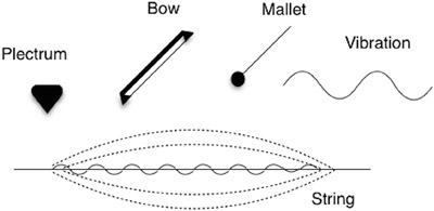
Figure 8.1 Various methods of exciting a string.
Physical Makeup
In addition to designating the material that strings are made of and the way in which they are excited, users will also be able to designate the material and physical properties that make up the body of the instrument. The physical makeup section of a PM synthesizer will usually have a huge amount of parameters that the user can adjust. Some examples of these parameters are the overall size of the instrument, the material it is made up of, how thick the instrument as a whole is, and, finally, the thickness of the material that makes up the instrument. Changing the physical attributes of the instrument’s body will drastically change the overall timbre of the sound.
Tuned Percussion Instruments
The next type of PM synthesizers we will examine model tuned percussion instruments. These instruments range from pianos to mallets and xylophones, all the way to tubular bells and beyond. As with the modeling of stringed instruments, PM synthesizers that model tuned percussion instruments will vary greatly between instruments. That being said, we will examine a few of the controls one might expect to run into.
Exciter Section
Like with stringed instruments, the exciter section of a tuned percussion PM synthesizer will designate what sets the instrument into vibration. Users will usually be able to choose between exciters such as beaters, mallets, hammers, and sticks as well as the material they are made up of. Users can designate the exciter with extreme precision and mix and match materials to make new types of exciters that might not be common in the physical world, such as metal mallets with felt tips. Additionally, it is not uncommon for users to designate not only the exciter’s material, but also how stiff it is.
Resonator Section
The next most common thing users will be able to determine on a PM-tuned percussion synthesizer is its resonator—or what is being set into vibration on the instrument. Choices for the user include strings, plates, beams, membranes, marimba beams, pipes, and tubes, as well as a variety of other, less common resonator sources. Like when modeling stringed instruments, changing the resonator material will result in drastic changes to the timbre of the sound.

Figure 8.2 Example of a resonator.
Nontuned Percussion Instruments
Tuned and nontuned percussion instruments are quite similar and oftentimes have a lot of overlap, but they merit a separate discussion. Nontuned percussion instruments involve drums, save for tom toms, cymbals, bongos, congas, and various other percussion instruments. Although individual drums can be “tuned,” they are typically not tuned to individual pitches and therefore are not considered tuned percussion instruments. Like with tuned percussion and stringed instruments, users will often be able to designate the material and stiffness of the exciter as well as the material and size of the resonator. Many PM percussion synthesizers will allow users to choose the material of the drum cavity as well as its inherent thickness.
Like with granular synthesis, many separate synthesis forms are lumped together under the phrase of physical modeling. These separate but related synthesis formats are waveguide synthesis; modal synthesis; McIntyre, Schumacher, and Woodhouse synthesis; Karplus-Strong synthesis; and formant synthesis. These other synthesis formats can be thought of as different approaches for physical modeling synthesis. Although they are all closely related, it is important to have a brief understanding of each format.

Figure 8.3 Digital waveguide synthesis attempts to mimic traveling sound waves through various mediums.
Waveguide Synthesis
Digital waveguide synthesis is a form of synthesis that attempts to mimic the way in which sound waves travel through a physical medium. For example, think of a clarinet. Once vibrations are created at the reed of a clarinet, sound waves propagate through the tube of the instrument. The material in which the clarinet is made of as well as which tone holes are open or closed, all play a part in the overall timbre of the instrument. Digital waveguide synthesis utilizes complex mathematical formulas in order to replicate these functions. In essence, a waveguide can be thought of as the medium that guides the wave, such as the tube and bell of a clarinet. Digital waveguide synthesis is used heavily in most physical modeling synthesizers in order to accurately replicate physical mediums.
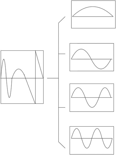
Figure 8.4 Modal synthesis focuses on the frequency domain of vibrating objects.
Modal Synthesis
Modal synthesis is one of the more complex techniques employed in physical modeling synthesis. Modal synthesis focuses on the frequency domain of a vibrating object. Modal synthesis can be crudely compared to additive or Fourier synthesis in that a vibrating object is deconstructed to base frequencies or modes that can then be analyzed and resynthesized. The formulas used in modal synthesis are complex and exist outside the scope of this book, but a basic understanding is helpful. In essence, modal synthesis is used to designate frequency information resultant of sound moving through various mediums. Returning back to the clarinet example, modal synthesis can be utilized to create a much more accurate representation of how pitch changes when tone holes are covered or opened. For this reason, modal synthesis is used heavily in physical modeling synthesizers.
McIntyre, Schumacher, and Woodhouse Synthesis
McIntyre, Schumacher, and Woodhouse synthesis, or MSW for short, is yet another technique employed in the modern physical modeling synthesizer. While modal synthesis focuses on the frequency domain of vibrating objects, MSW synthesis focusses on the time domain of vibrating objects. Again returning back to the clarinet, MSW synthesis focuses on the linear and nonlinear excitation resulting from the user blowing on the clarinet’s reed. An inherent pitch is present on any clarinet simply from the relation of the length of the instrument and the amount of blowing force applied to the reed. MSW synthesis is used to deconstruct this inherent pitch and then apply it to a resynthesized model.

Figure 8.5 MSW synthesis focuses on the time domain of vibrating objects.
Karplus-Strong Synthesis
Karplus-Strong synthesis is used in plucked string and drum PM synthesis. Karplus-Strong (KS) synthesis utilizes waveguide synthesis for its algorithms. KS synthesis uses complex waveguides at the onset of every note and then sharply diminishes the frequency content in quick succession. By starting with a complex set of frequencies and then quickly diminishing that amount, plucked string and drum sounds can be created quite accurately. When a violinist plucks a string, for example, the sound is extremely rich at the onset and then quickly falls to a much simpler, sine wave-like tone once the higher order harmonics fade away. KS synthesis attempts to mimic this through complex algorithms and formulas.

Figure 8.6 KS synthesis focuses on frequency and amplitude loss in plucked string over time.
Formant Synthesis
Formant synthesis involves passing signal through a number of complex resonant filters. In practice, formant synthesis is most often used in speech synthesis and creating vowel-type sounds. In its traditional sense, formant synthesis is not typically used outside of laboratories and universities. That being said, aspects of formant synthesis, such as formant filters, are used heavily in commercial physical modeling synthesis. Unlike the previous synthesis formats and algorithms examined, formant filters are used as a feature on PM synthesizers rather than a sound-generation source. Formant filters are often sought after for the unique and interesting sonic characteristics they impart on the overall sound.

Figure 8.7 Formant synthesis utilizes a series of filters known as formant filters to mimic individual formants found in acoustic instruments.
The Physical Modeling Model
These various synthesis techniques are all utilized to some extent in most modern physical modeling synthesizers. Because each technique is extremely well suited for its exact purpose, they all can be utilized to create an extremely powerful physical modeling synthesizer. Much like LEGO bricks, aspects of each of these formats can be used together in order to create a single instrument. Most PM synthesizers will not advertise that they use these types of algorithms nor will they offer the user the ability to turn on or off individual algorithms. Instead, all or most of these algorithms will be working “under the hood” of a PM synthesizer in order to create the complex and awesome sounds one desires.
Putting It All Together
Up to now, we have discussed the various attributes one can expect to find with a physical modeling synthesizer as well as the theory behind its numerous algorithms. In past chapters, once the discussion of individual parts is given, an explanation and examples are provided on how to build a sound from scratch. This is not the case with physical modeling synthesis. In reality, the algorithms used to achieve the breathtaking sounds physical modeling synthesis offers are just too complex to be useful to the average musician. Because of this, most physical modeling synthesizers will rely on factory presets as starting points and give users the ability to adjust certain parameters. Although this might seem prohibitive to some, it is really the only way in which physical modeling synthesis can be useful to the masses. So instead of starting new sounds completely from scratch, users will build up their sounds from the factory presets or factory default settings. Each PM synthesizer will allow for unique sound modification, but most users can expect to see a few standard parameter controls: including the ability to designate the material an instrument is made of, how the instrument is excited or played, and individual tensions and frictions of various parameters. Most PM synthesizers will also provide some standard synthesis adjustability such as pitch bending, modulation, and some type of filtering.
Every synthesis format discussed up until this point requires practice and patience in order to master it. Physical modeling synthesis is unique though in that it requires an extreme amount of practice to master. While most synthesizers can simply be plugged in and fiddled with to create useable sounds, PM synthesis requires extreme precision in order to create desirable sounds that are useful and not cheesy. Because PM synthesis emulates real instruments through algorithms representing physical attributes, extreme care must be taken when playing to ensure things like breath amount are interpreted as real sounding, rather than odd, digital artifacts. Sample-based synthesis is free from this challenge as things like breath noise is recorded into the samples. Unlike sample-based synthesis, PM synthesis requires the user to delicately add in things like breath noise when appropriate.
The amount of time and practice it takes to create realistic sounds using PM synthesis should not deter you. On the contrary, the time spent with a physical modeling instrument should be viewed as fun and engaging. To this day, despite all the advancements made in synthesis and sampling technology, physical modeling synthesis is still the most powerful way to emulate physical instruments. PM technology is still evolving and becoming better every time CPU power increases.
Hardware Physical Modeling Synthesizers
Now that we have discussed physical modeling synthesis and the technology behind it, let us examine some physical modeling synthesizers. By examining the various options users have when it comes to picking a PM synthesizer, we can explore some of the features unique to physical modeling synthesis.
Yamaha “VL” Line
Often cited as one of the earliest physical modeling synthesizers to hit the market, the VL-1 brought life back into the often stagnant and stock synthesizers of the day. With the VL-1, Yamaha introduced their own version of physical modeling technology, which they called Virtual Acoustic Technology. Yamaha shipped the VL-1s with a MIDI foot and breath controller to provide the most amount of control possible. With certain brass and woodwind patches, the breath controller would add more and more breath noise into the sound the harder one would blow. At extreme levels, pitch and timbre instability would arise that would oftentimes sound extremely musical and interesting. The VL-1 revolutionized the way in which musicians interacted with a synthesizer. For many users, playing the VL-1 made them feel that they were interacting with a real, physical instrument, rather than a keyboard-controlled computer: something that had not been felt since the days of analog subtractive synthesizers.
Due to the extreme complexity of the VL-1’s sound-generation engine, Yamaha did not provide the possibility for users to create their own patches from scratch. Instead, Yamaha included a wealth of customization capabilities that could be applied to the factory set sounds. The user adjustment options included:
- Pressure (bow speed)
- Scream (a type of controllable chaotic distortion)
- Tonguing (emulates tongue dampening of reeds)
- Amplitude
- Breath Noise
- Throat Formant (emulates effects of lungs, mouth, and throat)
- Damping (emulates friction)
- Growl (LFO effected pressure control)
- Dynamic Filter (filter cutoff adjustment)
- Harmonic Enhancer
- Embouchure (emulates the tightness of a players lips)
- Vibrato
- Absorption (emulates natural high frequency loss)
- Pitch (affects overall pitch of the instrument)
All of these parameters could be mapped to any MIDI controller, allowing for use with traditional sliders and knobs as well as foot and breath controllers. So although Yamaha did not allow users to create their own sounds completely from scratch, the sound could be dramatically changed from the factory presets. Despite the extreme attraction many people had towards the VL-1, it was extremely cost prohibitive to many people. Yamaha then released the VL-7, which was more affordable. Although slightly less powerful than its older sibling the VL-1, the VL-7 was widely adopted by people excited about physical modeling technology.
Technics SX-WSA1
The Technics SX-WSA1 synthesizer is an elaboration on physical modeling synthesis. The Technics SX-WSA1 uses what it calls acoustic modeling rather than physical modeling. Both acoustic and physical modeling are extremely similar and do not necessarily warrant separate names. The engineers at Technics decided that they wanted to create a more accessible physical modeling synthesizer. They felt that synthesizers like the Yamaha VL-1 were too complex and unintuitive to be useful. When creating the SX-WSA1, the physical modeling model was examined in depth and deconstructed in order to make it simpler. The engineers at Technics decided that in order to accurately emulate physical sounds, they could split sound into three parts: drivers, resonators, and modifiers.
According to Technics, drivers are what produce raw sound like a piano hammer hitting a string, or the reed of a clarinet vibrating. Moving on, resonators are what color the sound emitting from the driver. An example of a resonator is the body of a musical instrument. Finally, the modifier is what shapes and colors sounds—mainly a filter. By breaking sounds down into these three categories, the engineers at Technics believed they could create a synthesizer that used drivers, resonators, and modifiers to create emulations of physical instruments in a much more user-friendly manner than the physical modeling-monster synths that came before it.
The SX-WSA1 provided users with a large number of drivers (over three hundred), and tons of resonators. Users could then combine various drivers with various resonators in order to build sounds. For the first time, users were free to create sounds from the ground up rather than starting at factory presets. Although starting with premade drivers and resonators is not really starting completely from scratch, it was leaps and bounds more customizable than the Yamaha VL platform. The SX-WSA1 proved to be a quite successful synthesizer and the new approach it offered to physical modeling synthesis paved the way to the physical modeling soft synths we know and love today.
Software Physical Modeling Synthesizers
Due to the complex nature of physical modeling synthesis algorithms, as well as the number of computations that must be made instantaneously, a physical modeling synthesizer is really only as good as its computational power. Therefore, physical modeling synthesis really excels in a software or VST environment where it can harness the user’s computer for CPU power. There are a large number of software PM synthesizers on the market, so we will only discuss a few of them that offer unique and interesting features.
Ableton Live—Tension, Electric, Collision
Three physical modeling synthesizers are officially offered to Ableton Live users—Tension, Electric, and Collision. Tension acts as a physical modeling string synthesizer while Electric adheres to electric pianos and Collision focuses on drums and percussion. All three of these PM synthesizers are extremely powerful and are extremely impressive, especially when compared to their low price point.
Tension allows users to designate almost every attribute of a stringed instrument through a variety of PM algorithms. Using a similar Acoustic Modeling architecture to the Technics SX-WSA1, users adjust parameters of drivers, resonators, and modifiers. Starting with the drivers, Tension allows strings to be excited through the means of picking, bowing, plucking, or even being struck with a mallet or hammer. Next, users can choose the size, shape, thickness, and material of the body of the instrument. Combining various excitation and resonator models allows for anything from extremely accurate instrument emulation all the way to extremely bizarre and alien-type sounds. In addition to choosing drivers and resonators, users can also determine the amount of finger pressure applied to strings, as well as the amount of mechanical dampening from things like the felt on piano hammers.
Ableton’s Electric is a physical modeling synthesizer designed to emulate electric pianos such as the famed Rhodes and Wurlitzer electric pianos of the 1970s. Electric follows a similar model to Tension in that it is based off the Acoustic Modeling model found in the Technics SX-WSA1. Electric allows for a wealth of user-adjustable control that relates directly to electric pianos. Some parameters that are able to be adjusted are:
- Mallets (how the tines are struck)
- Tines (tone producing mechanism in electric pianos)
- Pickups (transducers that turn physical vibrations into electricity)
- Dampers (mechanism which stops the vibration of tines)
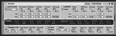
Figure 8.8 Ableton Live’s Tension PM string synthesizer.

Figure 8.9 Ableton Live’s Electric PM keyboard synthesizer.
Electric is capable of extremely accurate electric piano emulation and, in most instances, behaves more accurately than even some of the best sample libraries on the market. Electric even gives the user the ability to change the sound of the electric piano to emulate the way age affects the instrument.
Ableton’s final official physical modeling synthesizer is known as Collision. Collision is a drum and percussion emulation synthesizer that uses the same Acoustic Modeling model as Tension and Electric. Collision excels at mallet instruments such as marimbas, xylophones, and glockenspiels. Besides mallet instruments, Collision is capable of most drum and percussion emulation as well as some percussion stringed instruments like pianos and dulcimers. When programming on Collision, the user first selects the resonator, which in this case is both the physical playing surface as well as the resonating body. The choices of resonators are:
- Beam (emulates beams of different materials and sizes such as are found in xylophones)
- Marimba (form of beam that produces characteristic overtones of marimbas)
- String (emulates strings of varying size and material found in piano and dulcimers)
- Membrane (drum head with adjustments for material and size)
- Plate (acts as rectangular plate with adjustable material and size)
- Pipe (emulates a long cylinder with one open end and adjustable other end)
- Tube (emulates a long cylinder open at both ends)

Figure 8.10 Ableton Live’s Collision PM drum synthesizer.
Together, Tension, Electric, and Collision offer some of the best physical modeling synthesis options available on the market. The user control, playability, low price point, and overall sound quality are second to none. These three physical modeling synthesizers truly demonstrate the power PM synthesis offers.
Sculpture
Logic Pro’s Sculpture synthesizer is, in essence, an extremely powerful physical modeling and combination synthesizer (more on combination synthesis further in the chapter). When creating a sound in Sculpture, the first thing that must be determined is the material being used. Logic has introduced an exciting way of choosing materials in the form of a material square. The material square is a square in which each corner represents a different material—nylon, wood, steel, and glass. A ball is present in the square, which determines the material being heard, and can be moved at any point in the square allowing for any combination of the four materials imaginable. Besides just choosing the material of the instrument, Sculpture provides a huge number of exciters that range from traditional plucking and mallet strikes to symbiotic excitation.

Figure 8.11 Logic Pro’s Sculpture PM synthesizer.
Although Ableton Live’s Tension, Electric, and Collision PM synthesizers may be best suited for instrument emulation, Sculpture is best suited for creating new sounds via physical modeling synthesis. In fact, Sculpture is one of the first and only PM synthesizers designed to emulate not instruments themselves, but the way in which they interact with the environment. By focusing on individual aspects of physical instruments rather than the instrument as a whole, the user is free to create sounds completely unrestricted by the bounds of factory presets. Besides the extremely powerful physical modeling engine found on Sculpture, a few other features are present that make Sculpture even more powerful. To start with, Sculpture allows for a type of vector-like control over various aspects of the synthesizer. This vector-like control is known as Sculpture’s morph pad and it contains five points in which morph-able parameters can be routed to. Once parameters are routed to individual morph points, the user can manually drag the placement ball across the points and seamlessly move from one parameter setting to another. The placement ball can also be fully automated as well. Finally, Sculpture features some traditional synthesis capabilities such as filtering, LFOs, and envelope generators. Sculpture is an extremely powerful physical modeling synthesizer and is one of the most intuitive and creative software synthesizers available on the market today.
Analog Modeling
Another, perhaps more popular, version of physical modeling synthesis is available in the form of analog modeling synthesis. Analog modeling, sometimes referred to as virtual analog, is a derivative of physical modeling synthesis. As the analog resurgence began to sound in the 1990s and 2000s, many synthesizer companies felt the pressure to start producing analog synthesizers. Because of the uncertainty of how long the analog resurgence might last, as well as the difficulty of convincing shareholders to rehash old technologies, many synthesizer companies began offering analog modeling and virtual analog synthesizers as a compromise.
An analog modeling synthesizer will use many of the same techniques found in traditional physical modeling synthesizers. However, the goal of analog modeling synthesis is not just to re-create the sound of a particular analog synthesizer, but to mimic the way in which the individual analog components act. By mimicking the analog components rather than the overall timbre, analog modeling synthesizers are capable of creating much more realistic and believable sounds when compared to a digital subtractive synthesizer.
For example, one complaint many users have with digital subtractive synthesizers is the stepping heard when adjusting a parameter such as a filter’s cutoff frequency. This digital stepping is resultant of digital increments being cycled when performing a parameter sweep. In reference to the synthesizer’s filter, the filter can be heard opening or closing at small increments rather than a smooth transition as would be heard in an analog synthesizer.
By modeling the behaviors of the various analog components, analog modeling synthesizers can come much closer in sound to their analog counterparts. The algorithms used in analog modeling synthesis are designed to mimic circuitry behavior rather than physical property behavior like in traditional physical modeling synthesis.
Many hardware synthesizers, as well as VST plug-in synthesizers, have been released that use this analog modeling technology. Perhaps the most famous synthesizer to use analog modeling technology is the Clavia Nord line, such as the Nord Lead and Nord Modular synthesizers.

Figure 8.12 Filter responses on a digital subtractive synthesizer (right) and analog modeling synthesizer (left); notice the stepping present in the digital subtractive synth.

Figure 8.13 Clavia Nord Lead analog modeling synthesizer.
Released in 1995, the Clavia Nord Lead was a revolutionary new synthesizer that got a lot of people excited for the future of synthesis. The Nord Lead came at a time when subtractive synthesis was often overlooked and found only as afterthoughts on some combination digital synthesizers. For the first time in a long time, a hardware subtractive synthesizer was available that not only sounded great, but featured designated knobs for each parameter found on the synthesizer. The Nord Lead was capable of creating analog subtractive synth sounds, with full adjustability, without the hindrances of analog circuitry. The Nord Lead’s great sound was created solely through analog modeling technology.
Reminiscent of an analog subtractive synthesizer, the Clavia Nord Lead features two discreet oscillators, a multifilter, two envelope generators, a fully featured LFO, and an amplifier: in essence, full subtractive bliss. Many diehard analog users either covet or at least respect the Clavia Nord Lead thanks to the brilliant sounds that can be achieved all through the means of analog modeling technology.
Like the Clavia Nord Lead synthesizer, another influential synthesizer, the Access Virus, utilizes analog modeling as a sound generation engine. First released in 1997, the Access Virus line of synthesizers has gone on to enjoy wide acclaim. Both the Clavia Nord Lead synths as well as the Access Virus line of synths can be heard extensively on Nine Inch Nails tracks and newer Depeche Mode albums to name a few.
Even in the height of the analog synthesizer resurgence, new analog modeling synthesizers are being offered. Taking after the Nord Lead and Access Virus line of analog modeling synthesizers, Roland has entered the analog modeling market with their Aira line of synthesizers. Roland’s new Aira line uses what they call “Analog Circuit Behavior” technology. Roland’s “Analog Circuit Technology” is really just analog modeling technology with a higher number of individual algorithms. Nonetheless, the Aira line sound amazing and respond as if they are truly analog synthesizers. The Aira line consists of the flagship System-1 Synthesizer, TR-8 Rhythm Performer, TB-3 Touch Bassline, and the VT-3 Voice Transformer. Each of these synthesis devices are extremely powerful and display an incredible use of analog modeling technology. Roland also introduced a new “plug out” technology into the System-1 that allows users to perform a system dump of a VST synthesizer into the System-1’s memory so that it can be recalled without having to be connected to a computer. The Aria line of synthesizers and most notably the System-1 are an exciting direction for the analog modeling climate.
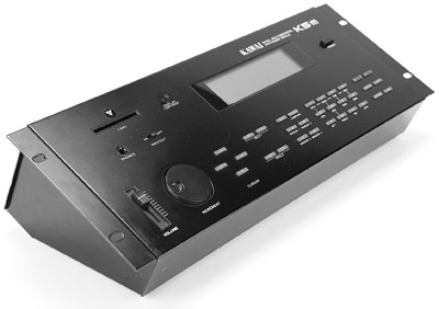
Figure 8.14 Access Virus analog modeling synthesizer.
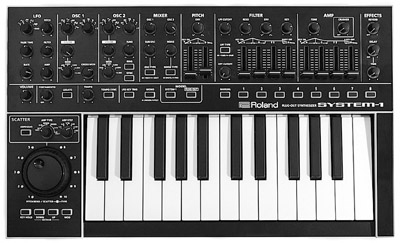
Figure 8.15 Roland Aira System-1 analog circuit behavior synthesizer.
Workstation and Combination Synthesizers
As digital recording became more prevalent in the 1990s, synthesist’s demands for synthesizers capable of being relevant in the digital recording studio became more widespread. As a response, companies like Roland, Yamaha, and Korg started producing workstation synthesizers. Workstation synthesizers are basically keyboards that feature a number of synthesis engines as well as multitrack recording and sampling capabilities. These workstation synthesizers will typically feature a number of synthesis engines such as subtractive, FM, sample based, etc. In addition to offering a number of sound synthesis engines, many workstation synthesizers will allow users to combine various elements of different synthesis engines. For example, a user could create a sound through FM synthesis, and then apply a resonant low pass filter such as is found on subtractive synthesizers. This ability to combine synthesis techniques is extremely attractive because it allows users to free themselves from the confines of a single synthesis format. The best attributes of each synthesis format can be combined in order to create one customized synthesizer that is perfectly suited for the user. Combination synthesis, as this combining functionality is termed, is found on most modern software synthesizers. Most software synthesizers will allow some sort of combination synthesis whether it is fully functional synthesis engines, or just a simple low pass filter.
The number of synthesizer workstations that have been released, and are subsequently on the new and used markets, could fill many chapters and do not warrant an in-depth model by model exploration. That being said, the Korg Kronos and Oasys are among the first workstation synthesizers and will serve to outline the features one might expect to find in a workstation and combination synthesizer.
Korg Kronos and Oasys
Both the Korg Kronos and the Oasys before it are powerful workstation synthesizers that boast nine discreet sound synthesis engines. The various synthesis engines available to Kronos and Oasys users include virtual subtractive synthesis, sample-based synthesis, physical modeling synthesis, wave shaping, and frequency modulation. The Oasys was Korg’s flagship workstation synthesizer up until the Kronos was introduced with better memory and greater computing power.
Besides just allowing for complex synthesis capabilities, the Kronos allows users to digitally record up to 16 tracks at 24-bit resolution as well as full MIDI connectivity. The trend of including digital recording capabilities on synthesizers became extremely widespread in the early 2000s and is still very much found today. Although widespread use of DAW software has somewhat eclipsed the usefulness of recording capabilities on workstation synthesizers, many users still desire the function ability.
Workstation Breakdown
Although what is desired in a workstation synthesizer is constantly changing, a few key elements will most likely be present in most, if not all, workstation synthesizers. These elements include a number of individual synthesis engines, as well as a complex sampling interface, both a complex sequencer and arpeggiator, multitrack digital audio recording interface, full MIDI connectivity, and, finally, a wealth of controller types including keys, sliders, knobs, and drum pads. In today’s ever-changing digital recording climate, the desire for workstation keyboards is dwindling. Multitype MIDI controllers seem to be replacing workstation synthesizers since they can easily be utilized in a DAW environment such as Logic Pro, FL Studio, or Ableton Live. Perhaps in an ironic twist of fate, all-in-one workstation synthesizers will regain popularity in the future and be coveted as “vintage synthesizers.”
Recipes
The recipes provided in this chapter will be geared towards physical modeling synthesis as it is the only completely unique synthesis format introduced in this chapter. For many years, the allure of modeling synthesis was its uncanny ability to re-create sounds with the utmost precision. Many people felt that this was modeling synthesis’s most prominent strength. Although modeling synthesis’s ability to re-create the sounds of physical instruments is astounding, we feel its true strength is its ability to create new sounds not attainable through any other form of synthesis. Therefore, we have chosen to take this direction in the creation of the recipes for this chapter. We chose to use the modeling soft synth Sculpture, which comes with the DAW Logic Pro. Before we delve into each of the recipes, let’s take some time to explore, in more depth, what Sculpture has to offer.
Sculpture
Sculpture is an immensely powerful modeling synthesizer. Besides its awe-inspiring modeling engine, Sculpture features a wealth of resonant filters, wave shaping capabilities, powerful DSP effects, and an immensely cool vector-inspired movement section. Add to this the powerful modulation matrix and various performance control features and Sculpture shines as a software synthesizer. To stay true to the modeling aspect of this chapter, we have chosen to create patches that only use Sculpture’s modeling engine. Therefore, traditional filters and effects will not be found in these recipes. Instead, the ten recipes that follow will serve to explore the sheer power that modeling synthesis has to offer. Before going through each of the recipes in depth, however, it is necessary to explain a few of the parameters we will be using inside of Sculpture.

Figure 8.16 Sculpture’s string section.
The String
Sculpture’s sound engine is based around the concept of a string. The entire synth is designed so that the user can determine the material this string is made of, how the string is excited into motion, how the string’s sound is captured, and then, finally, how the captured sound is modulated and effected. The circular section in the middle of the interface is where we can determine the material and stiffness of the string. Inside this circular section is a square labeled Material. By moving the sliver ball around this material square, we can determine the material the string is made up of. Our options are nylon, wood, steel, and glass. It is important to note, however, that similarly to a vector plane, this ball can be moved anywhere in this square allowing for an extreme amount of tonal changes.
Objects
Once we have determined the material of our string, we can choose up to three objects to excite said string. Each of the three objects has a wide variety of types, which relates to how the string will be excited. The range of types is vast but includes thing like bouncing, bow, strike, and impulse. All of these types are models. This means that if one were to choose the bouncing object type, Sculpture would produce an algorithm that mimicked something physically bouncing on the main string. The sounds that can be created with these models are truly breathtaking. You can think of these objects as oscillators with the type selector akin to a wave shape selector. Each object and type will add sonic character to the sound as a whole. We also have the ability to choose how the object responds to a key being pressed. We can choose to have the object excite the string either when a key is depressed, released, or have the object constantly exciting the string. A few additional options are available to us in which to further sculpt how the object will excite the string.

Figure 8.17 Sculpture’s object section.
Pickups and Object Positions
The Pickup section of Sculpture allows us to choose how we capture the sound emanating from the main string. Think of the two Pickups like pickups on a guitar, based off where the pickups are on a guitar’s body will determine the timbre of the sound. The two Pickups in Sculpture, A and B, can be separately moved across the entire length of the string. The two Pickup positions can also be modulated. Inside the Pickup section, we can find the object positions. These controls allow us to move each of the three objects to different areas of the string, causing different responses and timbres. Each of the three objects can be placed at any point on the string
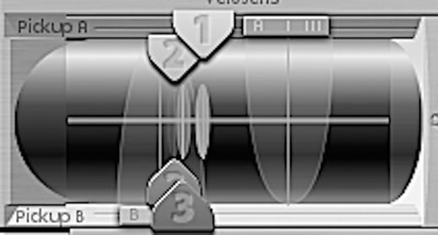
Figure 8.18 Sculpture’s Pickup and object position section.
LFOs and Modulation
Sculpture offers two freely assignable LFOs that can be routed to virtually any parameter on the synth, a third LFO dedicated to pitch modulation, or vibrato, two envelope generators, a jitter generator, and, finally, two randomizers. Each of these parameters can be sculpted by the user and routed to a variety of places for extreme modulation capabilities. The two main LFOs have a wealth of wave shapes and can be free running or beat synced.

Figure 8.19 Sculpture’s modulation section.
Master Section
The final parameter in Sculpture’s modeling engine is the Master section. In the Master section, we have the ability to adjust the main amplifier envelope generator as well as the panning of keys and Pickups, and then, finally, the overall level of the synth.
Other Parameters
As stated earlier, we are just focusing on the modeling engine inside of Sculpture, but there are a wealth of other parameters that Sculpture offers that warrant mention even though we will be disregarding them in our recipes. First and foremost is Sculpture’s powerful multifilter. Sculpture’s filter is fully resonant with high pass, low pass, peak, band pass, and notch filter shapes. Next is the wave shaper. Adjusting Sculpture’s wave shaper will add an amount of distortion or harshness to a patch that is quite astounding. Finally, a full-fledged morph pad and corresponding morph envelope allow for extreme amounts of animated movement, which is sure to take your patch to the next level.
Now that we have covered the basics of Sculpture’s modeling engine, let’s explore each of the patches we have created for this chapter. If you own Sculpture, feel free to follow along and expand upon these patches.

Figure 8.20 Sculpture’s Master section.
Recipe 1: Stiff Bouncing Shimmer
The first recipe on our list sounds like a soft mallet bouncing on the high strings of a piano. The sound is quite pretty and would fit well in most pop or ambient songs. The patch consists of all three objects with a string material that is between steel and nylon with about 60% resolution. Object one is set to Impulse with a keyOn gate. Object two is set to Bow with a KeyOn gate as well. Object three is set to Bouncing with a KeyOff gate so that the bouncing sound comes in once a key is released. Object one has about 75% strength while object two has 50% strength. Object three is weaker still, with about 20% strength. All the objects are placed in chronological order on the string with object one starting about 1/5th up the string from the left-hand side, while object three is about 4/6ths up the string. The amplifier’s envelope has zero attack with medium range decay and release and a slightly lower sustain. Both Key and Pickup are panned to the center. Pickup A is set at 1/4th up the string from the left while Pickup B is set at 3/4ths up the string from the left. A sine wave LFO set to 0.75Hz is routed to Pickup B’s pan control, almost fully engaged in the positive domain.

Figure 8.21 Screenshot of Stiff Bouncing Shimmer patch.

Figure 8.22 Screenshot of Distorted Dissonant Pop patch.
Recipe 2: Distorted Dissonant Pop
At first, this second recipe sounds like a distorted FM synth sound, but then it quickly turns dissonant in an extremely pleasing manner. The patch consists of just the first two objects both turned to Impulse. Object one has a strength setting of 100% while object two is set to 50% strength. The string material is fairly close to the Steel corner with full resolution. Object one is placed about 1/3rd up the string from the left, while object two is placed directly in the center. Pickup A is placed about 1/4th up the string from the left, while Pickup B is placed 3/4ths up the string. The Pickup parameter is spread modestly into the left and right while Key is fully spread. The amplifier envelope is set to an extremely short attack, midrange decay, full sustain, and nonexistent release. Finally, a 100Hz sine wave LFO is routed to the position of both Pickups with about 30% depth in the positive domain.
Recipe 3: Realistic Muted Bass
The third recipe on our list is extremely reminiscent of a slightly muted electric bass being played with a pick. The sound consists of the first two objects with a type setting of Impulse and Strike, respectively. Both objects feature about a 50% strength setting. The string material is set between steel and nylon with the setting close to nylon and about 60% resolution. Pickup A is placed about 1/5th up the string from the left while Pickup B is placed about 3/5ths up the string. Object one and two are placed on either side of the halfway mark with about a full 1/4th space between them. The amplifier envelope features an extremely short attack time, midrange decay time, full sustain, and about a 3/4ths full release time. The Pickup setting is fully spread.

Figure 8.23 Screen shot of Realistic Muted Bass patch.
Recipe 4: Odd Shimmering Pad
The fourth recipe on our list is a weird pad-type sound that can only be explained by imagining a steel bow scraping across a resonant steel sheet. The sound consists of all three objects with Strike, Blow, and Bouncing type settings respectively. Object one has a 50% strength setting, while objects two and three have a 25% setting. Object one is placed 3/4ths up the string from the left, while object two is placed 1/4ths up and object three placed about halfway up. Pickup A is in line with object two while Pickup B is placed directly before object one. The string material is set between steel and glass with the selector being closer to steel with full resolution. The amplifier envelope features a 3/4ths-full attack time, half-full decay, full sustain, and 3/4ths-full release. Both Key and Pickup are fully spread. A 6.70Hz sine wave LFO is routed to the panning of Pickup A and B with 100% positive depth, while a second 0.08 sine wave LFO is routed just to the panning of Pickup A with about a 50% positive depth.

Figure 8.24 Screenshot of Odd Shimmering Pad patch.
Recipe 5: Deep Synth Bass
The fifth recipe on our list is reminiscent of a traditional, eighties’ synth bass, but with a weird elastic rubber quality to it. The sound is made up of all three objects with Strike, Pick, and Bouncing settings respectively. Object one has a 100% strength setting, while both object two and three feature 50% strength settings. Object one is placed just shy of 3/4ths up the string from the left, while object two is placed 1/5th up and object three is almost directly between objects one and two. Pickup A is perfectly in line with object two, while Pickup B is perfectly in line with object one. The string material is between nylon and steel with heavy emphasis towards steel and full resolution. The amplifier envelope features an extremely short attack with a midrange decay, full sustain, and 3/4-full release.

Figure 8.25 Screenshot of Deep Synth Bass patch.
Recipe 6: Vibrating Bells
The sixth recipe on our list sounds a bit like if one were to gently strike bells with a felted mallet. The sound consists of the first two objects set to Impulse and Bow respectively. Object one features a strength setting of about 90%, while object two’s strength is set to about 75%. Object one is placed about 1/5th up the string from the left, while object two is placed 4/5ths up. Pickup A is perfectly in line with object one, while Pickup B is placed about 3/5ths up the string. The string material is between steel and glass but inching towards the middle of the plane, allowing for a slight mix between all the materials. The string features full resolution. The amplifier envelope features an extremely short attack, midrange decay, full sustain, and 3/4-full release. Key is slightly spread. A 0.19Hz sine wave LFO is routed to object two’s position with 100% positive depth. An additional 0.07Hz sine wave LFO is routed to the position of Pickups A and B with 100% positive depth.

Figure 8.26 Screenshot of Vibrating Bells patch.

Figure 8.27 Screenshot of Full Spectrum Synth patch.
Recipe 7: Full Spectrum Synth
This seventh recipe is a cool synthesized mix between a low guitar string pluck and high-end piano. It’s made up of just two objects with Impulse and Noise type settings, respectively. Object one is set to a KeyOn gate with 100% strength, while object two is set to a KeyOff gate with about 65% strength. Object one and two are both placed about 1/3rd up the string from the left with object one slightly further to the right than object two. Pickup B is slightly to the left of object two while Pickup A is about 3/4ths up the string from the left. The string material is in the bottom left corner, allowing for a mix between steel, glass, and nylon with most emphasis placed on steel. The string features full resolution. The amplifier envelope features an extremely short attack, almost full decay, zero sustain, and slightly more than half of a full release. Finally, a 0.12Hz triangle wave LFO is routed to the position of Pickups A and B with about 36% positive depth.
Recipe 8: High Rate of Wobble
The eighth recipe on our list sounds like an acoustic guitar being strummed under water. It’s made up of all three objects with Impulse, Noise, and Bouncing type settings, respectively. Object one features 100% strength setting, object two features 34% strength setting, and object three features 62% strength setting. Objects one and three are placed almost on top of one another about 1/3rd up the string from the left, while object two is placed 3/4ths up the string from the left. Pickup A is placed directly to the left of objects one and three, while Pickup B is placed directly to the left of object two. The string material is in the bottom left of the square resulting in a mixture between nylon, steel, and glass, with a heavy emphasis on steel. The string features full resolution. The amplifier envelope generator features an extremely short attack with almost full decay, nonexistent sustain, and a little more than half of a full release. The Pickup parameter is fully spread. A 31Hz triangle wave LFO is routed to the panning of Pickups A and B with 100% positive depth, which results in the underwater aspect of the sound.

Figure 8.28 Screenshot of High Rate of Wobble patch.
Recipe 9: Synth Keys
The ninth recipe on our list is reminiscent of an electric piano: only with a metallic, synthetic flair. The patch consists of only the first object engaged with a GravStrike type setting and a 75% strength setting with an Always gate. Object one is placed directly in the center of the string with Pickups A and B 1/4th in from either side of the string. The string material is in between nylon and steel, but much closer to steel. The selector ball for the string material is a bit inward in the plane, so a mix is able to be heard of all materials. The string also features a resolution of 100%. The amplifier envelope features an extremely short attack, full decay and sustain, and, finally, a 1/4th-full release. Pickup is fully spread. A 1/2-beat sine wave LFO is routed to the position of Pickups A and B with a 20% negative depth.

Figure 8.29 Screenshot of Synth Keys patch.
Recipe 10: Distant Rhythms
The final recipe on our list is one of the coolest. It’s a highly animated pad that sounds like an electronic music concert heard from outside of a tent. This patch was designed to be used in the lower register of a keyboard. This patch consists of only the first object engaged with a Noise type setting and about 50% strength. The timbre and variation settings on the object are both set at 100% in the positive direction. Object one is placed slightly to the left of center while Pickups A and B are both 1/6th in from either side of the string. The string material is almost fully set to steel with a 76% resolution. The amplifier attack is extremely short, while both the decay and sustain parameters are set to full. Release is set just shy of halfway. The Pickup parameter is almost fully spread. A 1/4 beat “Rect01” shaped LFO is routed to the positions of Pickups A and B as well as object one’s timbre. The routing to the Pickups has a 100% positive depth, while the object timbre routing has a 100% negative depth. This first LFO also features a 48% positive curve setting. The second LFO is a 1/8th-beat sawtooth LFO with a negative 16% curve setting. This LFO is routed to object one’s timbre as well, only with a 40% positive depth.

Figure 8.30 Screenshot of Distant Rhythms patch.
Historical Perspective on Modeling Synthesis
Like some of the other synthesis formats discussed in this book, physical modeling synthesis was conceived before the technology existed with which to implement it. The first strides in physical modeling synthesis came from Lejaren Hiller and Pierre Ruiz. Hiller and Ruiz, who worked out of the State University of New York and Bell Laboratories, respectively, conceived of a way of creating realistic models of physical instruments through using finite difference approximations of the wave equation.1 In essence, Hiller and Ruiz examined vibrating objects, such as strings, and attempted to describe them via differential equations that could then be coded and programmed for a digital computer. Although Hiller and Ruiz only concentrated on vibrating strings, they were able to prove their methods for use with other vibrating objects such as bars, plates, membranes, and spheres. Although Hiller and Ruiz were able to successfully model limited stringed instruments, it was not until the development of the Karplus-Strong algorithm that physical modeling synthesis started to gain traction in the scientific world.2
Alexander Strong invented, while Kevin Karplus analyzed and described, the algorithm that would become known as the Karplus-Strong algorithm. The algorithm models the sound of a plucked or hammered string by looping a short waveform through a filtered delay line. Imagine a plucked string, such as a cello played in a pizzicato manner. Directly after the string is plucked, the sound will be harmonically rich. Shortly after the string is first plucked, however, the higher harmonics will start to drop in amplitude followed by the lower harmonics, until the sound is finally inaudible. When using the Karplus-Strong algorithm, a short waveform is produced and then looped back into a low pass filter, eliminating some of the higher frequencies. The new, filtered waveform is looped back into the filter and more high harmonics are filtered out of the sound. The resulting waveforms are continuously looped and filtered until the sound is inaudible, mimicking the way in which a plucked string would naturally fade away. Each loop corresponds to approximately one period, or cycle, of the waveform.
The introduction and success of the Karplus-Strong algorithm piqued the interest of a lot of engineers and synthesizer companies. Brief murmurings about the promise of this new technology could be heard among a few, select individuals. One such person was Julius Smith, who went on to create an extension of the Karplus-Strong algorithm, which would become known as digital waveguide synthesis.3 Digital waveguides are basically computational models for the way in which acoustic waves move through physical media. Using waveguide synthesis, engineers were able to successfully model a number of instruments with extreme accuracy.
Although the theory was there, DSP power simply was not. It would not be long, however, until DSP power would catch up with physical modeling theory and begin being implemented in commercial instruments. Yamaha was one of the first companies to see the potential of physical modeling synthesis. In 1989, Yamaha signed a contract with Stanford University to begin designing instruments that would feature this new technology. The first such instrument to utilize physical modeling synthesis was the Yamaha VL-1 released in 1994. The VL-1 was a revolutionary instrument that held extreme promise. Although many people were able to realize the sheer power of VL-1, it was far out of the reach of many people’s budgets. In order to try and bring more appeal to Yamaha’s new synthesis technology, the company released the VL-7, which was a slightly scaled back but much less expensive version of the VL-1. The VL-7 proved to be quite successful and even encouraged more manufacturers to release their own physical modeling synthesizers. However, sampling technology and low budget rompler synthesizers overshadowed the much more powerful physical modeling synthesizers of the day, resulting in a declining number of sales.
Physical modeling technology would, more or less, stay dormant throughout the 1990s and early 2000s. Although the occasional physical modeling sound engine would show up in a workstation synthesizer every now and again, no worthwhile advancements were made in the technology. This all started to change with the coming of digital audio workstations and software-based synthesis engines. CPU power began to reach levels that allowed for extremely powerful synthesis engines without much computational strains. Physical modeling synthesis has since flourished in the software domain with programs such as Reason and Ableton Live offering users a wealth of physical modeling capabilities.
Physical modeling synthesis is often confused with sample- based synthesis and is often overlooked and disregarded. Because of the extreme realism that can be achieved using physical modeling synthesis, many people just assume it to be interchangeable with sample-based synthesis. This viewpoint, however, fails to realize the power physical modeling synthesis holds as an independent synthesis engine. The truth is that physical modeling synthesis can not only re-create physical instruments beautifully, it can create new and interesting sounds that do not exist outside the world of physical modeling synthesis. Because of this, physical modeling synthesis should never be overlooked and should, instead, be realized for what it is, an amazing and truly inspiring synthesis format.
Notes
1.Diana Deutsch, The Psychology of Music, San Diego, CA: Gulf Professional Publishing, 1999, pp. 132.
2.J. O. Smith, “Delay Lines,” in Physical Audio Signal Processing, http://ccrma.stanford.edu/~jos/pasp/Delay_Lines.html, online book, 2010 edition.
3.Julius O. Smith, III, “Physical Modeling using Digital Waveguides,” Computer Music Journal vol. 16, no. 4 (Winter 1992), pp. 74–91.