Overview
This chapter will show you how to train a multiclass classifier using the Random Forest algorithm. You will also see how to evaluate the performance of multiclass models.
By the end of the chapter, you will be able to implement a Random Forest classifier, as well as tune hyperparameters in order to improve model performance.
Introduction
In the previous chapter, you saw how to build a binary classifier using the famous Logistic Regression algorithm. A binary classifier can only take two different values for its response variables, such as 0 and 1 or yes and no. A multiclass classification task is just an extension. Its response variable can have more than two different values.
In the data science industry, quite often you will face multiclass classification problems. For example, if you were working for Netflix or any other streaming platform, you would have to build a model that could predict the user rating for a movie based on key attributes such as genre, duration, or cast. A potential list of rating values may be: Hate it, Dislike it, Neutral, Like it, Love it. The objective of the model would be to predict the right rating from those five possible values.
Multiclass classification doesn't always mean the response variable will be text. In some datasets, the target variable may be encoded into a numerical form. Taking the same example as discussed, the rating may be coded from 1 to 5: 1 for Hate it, 2 for Dislike it, 3 for Neutral, and so on. So, it is important to understand the meaning of this response variable first before jumping to the conclusion that this is a regression problem.
In the next section, we will be looking at training our first Random Forest classifier.
Training a Random Forest Classifier
In this chapter, we will use the Random Forest algorithm for multiclass classification. There are other algorithms on the market, but Random Forest is probably one of the most popular for such types of projects.
The Random Forest methodology was first proposed in 1995 by Tin Kam Ho but it was first developed by Leo Breiman in 2001.
So Random Forest is not really a recent algorithm per se. It has been in use for almost two decades already. But its popularity hasn't faded, thanks to its performance and simplicity.
For the examples in this chapter, we will be using a dataset called "Activity Recognition system based on Multisensor data." It was originally shared by F. Palumbo, C. Gallicchio, R. Pucci, and A. Micheli, Human activity recognition using multisensor data fusion based on Reservoir Computing, Journal of Ambient Intelligence and Smart Environments, 2016, 8 (2), pp. 87-107.
Note
The complete dataset can be found here: https://packt.live/3a5FI1s
Let's see how we can train a Random Forest classifier on this dataset. First, we need to load the data from the GitHub repository using pandas and then we will print its first five rows using the head() method.
Note
All the example code given outside of Exercises in this chapter relates to this Activity Recognition dataset. It is recommended that all code from these examples is entered and run in a single Google Colab Notebook, and kept separate from your Exercise Notebooks.
import pandas as pd
file_url = 'https://raw.githubusercontent.com/PacktWorkshops'
'/The-Data-Science-Workshop/master/Chapter04/'
'Dataset/activity.csv'
df = pd.read_csv(file_url)
df.head()
The output will be as follows:

Figure 4.1: First five rows of the dataset
Each row represents an activity that was performed by a person and the name of the activity is stored in the Activity column. There are seven different activities in this variable: bending1, bending2, cycling, lying, sitting, standing, and Walking. The other six columns are different measurements taken from sensor data.
In this example, you will accurately predict the target variable ('Activity') from the features (the six other columns) using Random Forest. For example, for the first row of the preceding example, the model will receive the following features as input and will predict the 'bending1' class:

Figure 4.2: Features for the first row of the dataset
But before that, we need to do a bit of data preparation. The sklearn package (we will use it to train Random Forest model) requires the target variable and the features to be separated. So, we need to extract the response variable using the .pop() method from pandas. The .pop() method extracts the specified column and removes it from the DataFrame:
target = df.pop('Activity')
Now the response variable is contained in the variable called target and all the features are in the DataFrame called df.
Now we are going to split the dataset into training and testing sets. The model uses the training set to learn relevant parameters in predicting the response variable. The test set is used to check whether a model can accurately predict unseen data. We say the model is overfitting when it has learned the patterns relevant only to the training set and makes incorrect predictions about the testing set. In this case, the model performance will be much higher for the training set compared to the testing one. Ideally, we want to have a very similar level of performance for the training and testing sets. This topic will be covered in more depth in Chapter 7, The Generalization of Machine Learning Models.
The sklearn package provides a function called train_test_split() to randomly split the dataset into two different sets. We need to specify the following parameters for this function: the feature and target variables, the ratio of the testing set (test_size), and random_state in order to get reproducible results if we have to run the code again:
from sklearn.model_selection import train_test_split
X_train, X_test, y_train, y_test = train_test_split
(df, target, test_size=0.33,
random_state=42)
There are four different outputs to the train_test_split() function: the features for the training set, the target variable for the training set, the features for the testing set, and its target variable.
Now that we have got our training and testing sets, we are ready for modeling. Let's first import the RandomForestClassifier class from sklearn.ensemble:
from sklearn.ensemble import RandomForestClassifier
Now we can instantiate the Random Forest classifier with some hyperparameters. Remember from Chapter 1, Introduction to Data Science in Python, a hyperparameter is a type of parameter the model can't learn but is set by data scientists to tune the model's learning process. This topic will be covered more in depth in Chapter 8, Hyperparameter Tuning. For now, we will just specify the random_state value. We will walk you through some of the key hyperparameters in the following sections:
rf_model = RandomForestClassifier(random_state=1,
n_estimators=10)
The next step is to train (also called fit) the model with the training data. During this step, the model will try to learn the relationship between the response variable and the independent variables and save the parameters learned. We need to specify the features and target variables as parameters:
rf_model.fit(X_train, y_train)
The output will be as follows:

Figure 4.3: Logs of the trained RandomForest
Now that the model has completed its training, we can use the parameters it learned to make predictions on the input data we will provide. In the following example, we are using the features from the training set:
preds = rf_model.predict(X_train)
Now we can print these predictions:
preds
The output will be as follows:

Figure 4.4: Predictions of the RandomForest algorithm on the training set
This output shows us the model predicted, respectively, the values lying, bending1, and cycling for the first three observations and cycling, bending1, and standing for the last three observations. Python, by default, truncates the output for a long list of values. This is why it shows only six values here.
These are basically the key steps required for training a Random Forest classifier. This was quite straightforward, right? Training a machine learning model is incredibly easy but getting meaningful and accurate results is where the challenges lie. In the next section, we will learn how to assess the performance of a trained model.
Evaluating the Model's Performance
Now that we know how to train a Random Forest classifier, it is time to check whether we did a good job or not. What we want is to get a model that makes extremely accurate predictions, so we need to assess its performance using some kind of metric.
For a classification problem, multiple metrics can be used to assess the model's predictive power, such as F1 score, precision, recall, or ROC AUC. Each of them has its own specificity and depending on the projects and datasets, you may use one or another.
In this chapter, we will use a metric called accuracy score. It calculates the ratio between the number of correct predictions and the total number of predictions made by the model:

Figure 4.5: Formula for accuracy score
For instance, if your model made 950 correct predictions out of 1,000 cases, then the accuracy score would be 950/1000 = 0.95. This would mean that your model was 95% accurate on that dataset. The sklearn package provides a function to calculate this score automatically and it is called accuracy_score(). We need to import it first:
from sklearn.metrics import accuracy_score
Then, we just need to provide the list of predictions for some observations and the corresponding true value for the target variable. Using the previous example, we will use the y_train and preds variables, which respectively contain the response variable (also known as the target) for the training set and the corresponding predictions made by the Random Forest model. We will reuse the predictions from the previous section – preds:
accuracy_score(y_train, preds)
The output will be as follows:
Figure 4.6: Accuracy score on the training set
We achieved an accuracy score of 0.988 on our training data. This means we accurately predicted more than 98% of these cases. Unfortunately, this doesn't mean you will be able to achieve such a high score for new, unseen data. Your model may have just learned the patterns that are only relevant to this training set, and in that case, the model will overfit.
If we take the analogy of a student learning a subject for a semester, they could memorize by heart all the textbook exercises but when given a similar but unseen exercise, they wouldn't be able to solve it. Ideally, the student should understand the underlying concepts of the subject and be able to apply that learning to any similar exercises. This is exactly the same for our model: we want it to learn the generic patterns that will help it to make accurate predictions even on unseen data.
But how can we assess the performance of a model for unseen data? Is there a way to get that kind of assessment? The answer to these questions is yes.
Remember, in the last section, we split the dataset into training and testing sets. We used the training set to fit the model and assess its predictive power on it. But it hasn't seen the observations from the testing set at all, so we can use it to assess whether our model is capable of generalizing unseen data. Let's calculate the accuracy score for the testing set:
test_preds = rf_model.predict(X_test)
accuracy_score(y_test, test_preds)
The output will be as follows:
Figure 4.7: Accuracy score on the testing set
OK. Now the accuracy has dropped drastically to 0.77. The difference between the training and testing sets is quite big. This tells us our model is actually overfitting and learned only the patterns relevant to the training set. In an ideal case, the performance of your model should be equal or very close to equal for those two sets.
In the next sections, we will look at tuning some Random Forest hyperparameters in order to reduce overfitting.
Exercise 4.01: Building a Model for Classifying Animal Type and Assessing Its Performance
In this exercise, we will train a Random Forest classifier to predict the type of an animal based on its attributes and check its accuracy score:
Note
The dataset we will be using is the Zoo Data Set shared by Richard S. Forsyth: https://packt.live/36DpRVK. The CSV version of this dataset can be found here: https://packt.live/37RWGhF.
- Open a new Colab notebook.
- Import the pandas package:
import pandas as pd
- Create a variable called file_url that contains the URL of the dataset:
file_url = 'https://raw.githubusercontent.com'
'/PacktWorkshops/The-Data-Science-Workshop'
'/master/Chapter04/Dataset'
'/openml_phpZNNasq.csv'
- Load the dataset into a DataFrame using the .read_csv() method from pandas:
df = pd.read_csv(file_url)
- Print the first five rows of the DataFrame:
df.head()
You should get the following output:
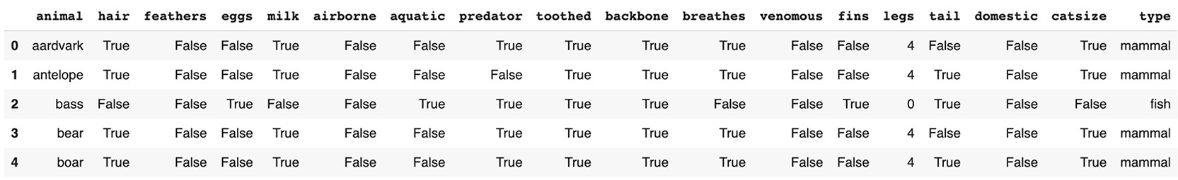
Figure 4.8: First five rows of the DataFrame
We will be using the type column as our target variable. We will need to remove the animal column from the DataFrame and only use the remaining columns as features.
- Remove the 'animal' column using the .drop() method from pandas and specify the columns='animal' and inplace=True parameters (to directly update the original DataFrame):
df.drop(columns='animal', inplace=True)
- Extract the 'type' column using the .pop() method from pandas:
y = df.pop('type')
- Print the first five rows of the updated DataFrame:
df.head()
You should get the following output:
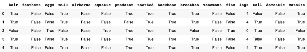
Figure 4.9: First five rows of the DataFrame
- Import the train_test_split function from sklearn.model_selection:
from sklearn.model_selection import train_test_split
- Split the dataset into training and testing sets with the df, y, test_size=0.4, and random_state=188 parameters:
X_train, X_test, y_train, y_test = train_test_split
(df, y, test_size=0.4,
random_state=188)
- Import RandomForestClassifier from sklearn.ensemble:
from sklearn.ensemble import RandomForestClassifier
- Instantiate the RandomForestClassifier object with random_state equal to 42. Set the n-estimators value to an initial default value of 10. We'll discuss later how changing this value affects the result.
rf_model = RandomForestClassifier(random_state=42,
n_estimators=10)
- Fit RandomForestClassifier with the training set:
rf_model.fit(X_train, y_train)
You should get the following output:
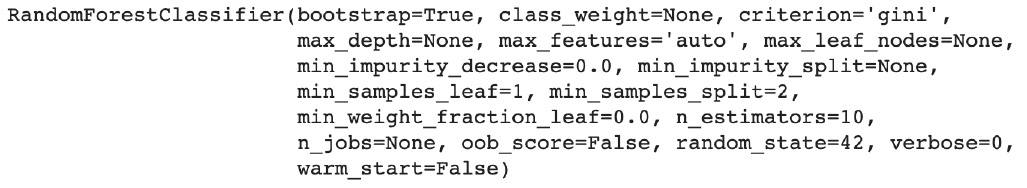
Figure 4.10: Logs of RandomForestClassifier
- Predict the outcome of the training set with the .predict()method, save the results in a variable called 'train_preds', and print its value:
train_preds = rf_model.predict(X_train)
train_preds
You should get the following output:

Figure 4.11: Predictions on the training set
- Import the accuracy_score function from sklearn.metrics:
from sklearn.metrics import accuracy_score
- Calculate the accuracy score on the training set, save the result in a variable called train_acc, and print its value:
train_acc = accuracy_score(y_train, train_preds)
print(train_acc)
You should get the following output:

Figure 4.12: Accuracy score on the training set
Our model achieved an accuracy of 1 on the training set, which means it perfectly predicted the target variable on all of those observations. Let's check the performance on the testing set.
- Predict the outcome of the testing set with the .predict() method and save the results into a variable called test_preds:
test_preds = rf_model.predict(X_test)
- Calculate the accuracy score on the testing set, save the result in a variable called test_acc, and print its value:
test_acc = accuracy_score(y_test, test_preds)
print(test_acc)
You should get the following output:

Figure 4.13: Accuracy score on the testing set
In this exercise, we trained a RandomForest to predict the type of animals based on their key attributes. Our model achieved a perfect accuracy score of 1 on the training set but only 0.88 on the testing set. This means our model is overfitting and is not general enough. The ideal situation would be for the model to achieve a very similar, high-accuracy score on both the training and testing sets.
Note
To access the source code for this specific section, please refer to https://packt.live/2Q4jpQK.
You can also run this example online at https://packt.live/3h6JieL.
Number of Trees Estimator
Now that we know how to fit a Random Forest classifier and assess its performance, it is time to dig into the details. In the coming sections, we will learn how to tune some of the most important hyperparameters for this algorithm. As mentioned in Chapter 1, Introduction to Data Science in Python, hyperparameters are parameters that are not learned automatically by machine learning algorithms. Their values have to be set by data scientists. These hyperparameters can have a huge impact on the performance of a model, its ability to generalize to unseen data, and the time taken to learn patterns from the data.
The first hyperparameter you will look at in this section is called n_estimators. This hyperparameter is responsible for defining the number of trees that will be trained by the RandomForest algorithm.
Before looking at how to tune this hyperparameter, we need to understand what a tree is and why it is so important for the RandomForest algorithm.
A tree is a logical graph that maps a decision and its outcomes at each of its nodes. Simply speaking, it is a series of yes/no (or true/false) questions that lead to different outcomes.
A leaf is a special type of node where the model will make a prediction. There will be no split after a leaf. A single node split of a tree may look like this:
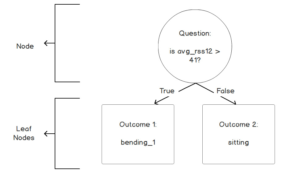
Figure 4.14: Example of a single tree node
A tree node is composed of a question and two outcomes depending on whether the condition defined by the question is met or not. In the preceding example, the question is is avg_rss12 > 41? If the answer is yes, the outcome is the bending_1 leaf and if not, it will be the sitting leaf.
A tree is just a series of nodes and leaves combined together:

Figure 4.15: Example of a tree
In the preceding example, the tree is composed of three nodes with different questions. Now, for an observation to be predicted as sitting, it will need to meet the conditions: avg_rss13 <= 41, var_rss > 0.7, and avg_rss13 <= 16.25.
The RandomForest algorithm will build this kind of tree based on the training data it sees. We will not go through the mathematical details about how it defines the split for each node but, basically, it will go through every column of the dataset and see which split value will best help to separate the data into two groups of similar classes. Taking the preceding example, the first node with the avg_rss13 > 41 condition will help to get the group of data on the left-hand side with mostly the bending_1 class. The RandomForest algorithm usually builds several of this kind of tree and this is the reason why it is called a forest.
As you may have guessed now, the n_estimators hyperparameter is used to specify the number of trees the RandomForest algorithm will build. For example (as in the previous exercise), say we ask it to build 10 trees. For a given observation, it will ask each tree to make a prediction. Then, it will average those predictions and use the result as the final prediction for this input. For instance, if, out of 10 trees, 8 of them predict the outcome sitting, then the RandomForest algorithm will use this outcome as the final prediction.
Note
If you don't pass in a specific n_estimators hyperparameter, it will use the default value. The default depends on the version of scikit-learn you're using. In early versions, the default value is 10. From version 0.22 onwards, the default is 100. You can find out which version you are using by executing the following code:
import sklearn
sklearn.__version__
For more information, see here: https://scikit-learn.org/stable/modules/generated/sklearn.ensemble.RandomForestClassifier.html
In general, the higher the number of trees is, the better the performance you will get. Let's see what happens with n_estimators = 2 on the Activity Recognition dataset:
rf_model2 = RandomForestClassifier(random_state=1,
n_estimators=2)
rf_model2.fit(X_train, y_train)
preds2 = rf_model2.predict(X_train)
test_preds2 = rf_model2.predict(X_test)
print(accuracy_score(y_train, preds2))
print(accuracy_score(y_test, test_preds2))
The output will be as follows:

Figure 4.16: Accuracy of RandomForest with n_estimators = 2
As expected, the accuracy is significantly lower than the previous example with n_estimators = 10. Let's now try with 50 trees:
rf_model3 = RandomForestClassifier(random_state=1,
n_estimators=50)
rf_model3.fit(X_train, y_train)
preds3 = rf_model3.predict(X_train)
test_preds3 = rf_model3.predict(X_test)
print(accuracy_score(y_train, preds3))
print(accuracy_score(y_test, test_preds3))
The output will be as follows:

Figure 4.17: Accuracy of RandomForest with n_estimators = 50
With n_estimators = 50, we respectively gained 1% and 2% on the accuracy scored for the training and testing sets, which is great. But the main drawback of increasing the number of trees is that it requires more computational power. So, it will take more time to train a model. In a real project, you will need to find the right balance between performance and training duration.
Exercise 4.02: Tuning n_estimators to Reduce Overfitting
In this exercise, we will train a Random Forest classifier to predict the type of an animal based on its attributes and will try two different values for the n_estimators hyperparameter:
We will be using the same zoo dataset as in the previous exercise.
- Open a new Colab notebook.
- Import the pandas package, train_test_split, RandomForestClassifier, and accuracy_score from sklearn:
import pandas as pd
from sklearn.model_selection import train_test_split
from sklearn.ensemble import RandomForestClassifier
from sklearn.metrics import accuracy_score
- Create a variable called file_url that contains the URL to the dataset:
file_url = 'https://raw.githubusercontent.com'
'/PacktWorkshops/The-Data-Science-Workshop'
'/master/Chapter04/Dataset'
'/openml_phpZNNasq.csv'
- Load the dataset into a DataFrame using the .read_csv() method from pandas:
df = pd.read_csv(file_url)
- Remove the animal column using .drop() and then extract the type target variable into a new variable called y using .pop():
df.drop(columns='animal', inplace=True)
y = df.pop('type')
- Split the data into training and testing sets with train_test_split() and the test_size=0.4 and random_state=188 parameters:
X_train, X_test, y_train, y_test = train_test_split
(df, y, test_size=0.4,
random_state=188)
- Instantiate RandomForestClassifier with random_state=42 and n_estimators=1, and then fit the model with the training set:
rf_model = RandomForestClassifier(random_state=42,
n_estimators=1)
rf_model.fit(X_train, y_train)
You should get the following output:
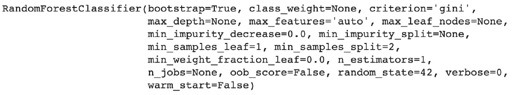
Figure 4.18: Logs of RandomForestClassifier
- Make predictions on the training and testing sets with .predict() and save the results into two new variables called train_preds and test_preds:
train_preds = rf_model.predict(X_train)
test_preds = rf_model.predict(X_test)
- Calculate the accuracy score for the training and testing sets and save the results in two new variables called train_acc and test_acc:
train_acc = accuracy_score(y_train, train_preds)
test_acc = accuracy_score(y_test, test_preds)
- Print the accuracy scores: train_acc and test_acc:
print(train_acc)
print(test_acc)
You should get the following output:

Figure 4.19: Accuracy scores for the training and testing sets
The accuracy score decreased for both the training and testing sets. But now the difference is smaller compared to the results from Exercise 4.01, Building a Model for Classifying Animal Type and Assessing Its Performance.
- Instantiate another RandomForestClassifier with random_state=42 and n_estimators=30, and then fit the model with the training set:
rf_model2 = RandomForestClassifier(random_state=42,
n_estimators=30)
rf_model2.fit(X_train, y_train)
You should get the following output:
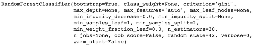
Figure 4.20: Logs of RandomForest with n_estimators = 30
- Make predictions on the training and testing sets with .predict() and save the results into two new variables called train_preds2 and test_preds2:
train_preds2 = rf_model2.predict(X_train)
test_preds2 = rf_model2.predict(X_test)
- Calculate the accuracy score for the training and testing sets and save the results in two new variables called train_acc2 and test_acc2:
train_acc2 = accuracy_score(y_train, train_preds2)
test_acc2 = accuracy_score(y_test, test_preds2)
- Print the accuracy scores: train_acc and test_acc:
print(train_acc2)
print(test_acc2)
You should get the following output:

Figure 4.21: Accuracy scores for the training and testing sets
This output shows us the model is overfitting less compared to the results from the previous step and still has a very high-performance level for the training set.
In the previous exercise, we achieved an accuracy score of 1 for the training set and 0.88 for the testing one. In this exercise, we trained two additional Random Forest models with n_estimators = 1 and 30. The model with the lowest number of trees has the lowest accuracy: 0.92 (training) and 0.8 (testing). On the other hand, increasing the number of trees to 30, we achieved a higher accuracy: 1 and 0.9. Our model is overfitting slightly less now. It is not perfect, but it is a good start.
Note
To access the source code for this specific section, please refer to https://packt.live/322x8gz.
You can also run this example online at https://packt.live/313gUV8.
Maximum Depth
In the previous section, we learned how Random Forest builds multiple trees to make predictions. Increasing the number of trees does improve model performance but it usually doesn't help much to decrease the risk of overfitting. Our model in the previous example is still performing much better on the training set (data it has already seen) than on the testing set (unseen data).
So, we are not confident enough yet to say the model will perform well in production. There are different hyperparameters that can help to lower the risk of overfitting for Random Forest and one of them is called max_depth.
This hyperparameter defines the depth of the trees built by Random Forest. Basically, it tells Random Forest model, how many nodes (questions) it can create before making predictions. But how will that help to reduce overfitting, you may ask. Well, let's say you built a single tree and set the max_depth hyperparameter to 50. This would mean that there would be some cases where you could ask 49 different questions (the value c includes the final leaf node) before making a prediction. So, the logic would be IF X1 > value1 AND X2 > value2 AND X1 <= value3 AND … AND X3 > value49 THEN predict class A.
As you can imagine, this is a very specific rule. In the end, it may apply to only a few observations in the training set, with this case appearing very infrequently. Therefore, your model would be overfitting. By default, the value of this max_depth parameter is None, which means there is no limit set for the depth of the trees.
What you really want is to find some rules that are generic enough to be applied to bigger groups of observations. This is why it is recommended to not create deep trees with Random Forest. Let's try several values for this hyperparameter on the Activity Recognition dataset: 3, 10, and 50:
rf_model4 = RandomForestClassifier(random_state=1,
n_estimators=50, max_depth=3)
rf_model4.fit(X_train, y_train)
preds4 = rf_model4.predict(X_train)
test_preds4 = rf_model4.predict(X_test)
print(accuracy_score(y_train, preds4))
print(accuracy_score(y_test, test_preds4))
You should get the following output:

Figure 4.22: Accuracy scores for the training and testing sets and a max_depth of 3
For a max_depth of 3, we got extremely similar results for the training and testing sets but the overall performance decreased drastically to 0.61. Our model is not overfitting anymore, but it is now underfitting; that is, it is not predicting the target variable very well (only in 61% of cases). Let's increase max_depth to 10:
rf_model5 = RandomForestClassifier(random_state=1,
n_estimators=50,
max_depth=10)
rf_model5.fit(X_train, y_train)
preds5 = rf_model5.predict(X_train)
test_preds5 = rf_model5.predict(X_test)
print(accuracy_score(y_train, preds5))
print(accuracy_score(y_test, test_preds5))

Figure 4.23: Accuracy scores for the training and testing sets and a max_depth of 10
The accuracy of the training set increased and is relatively close to the testing set. We are starting to get some good results, but the model is still slightly overfitting. Now we will see the results for max_depth = 50:
rf_model6 = RandomForestClassifier(random_state=1,
n_estimators=50,
max_depth=50)
rf_model6.fit(X_train, y_train)
preds6 = rf_model6.predict(X_train)
test_preds6 = rf_model6.predict(X_test)
print(accuracy_score(y_train, preds6))
print(accuracy_score(y_test, test_preds6))
The output will be as follows:

Figure 4.24: Accuracy scores for the training and testing sets and a max_depth of 50
The accuracy jumped to 0.99 for the training set but it didn't improve much for the testing set. So, the model is overfitting with max_depth = 50. It seems the sweet spot to get good predictions and not much overfitting is around 10 for the max_depth hyperparameter in this dataset.
Exercise 4.03: Tuning max_depth to Reduce Overfitting
In this exercise, we will keep tuning our RandomForest classifier that predicts animal type by trying two different values for the max_depth hyperparameter:
We will be using the same zoo dataset as in the previous exercise.
- Open a new Colab notebook.
- Import the pandas package, train_test_split, RandomForestClassifier, and accuracy_score from sklearn:
import pandas as pd
from sklearn.model_selection import train_test_split
from sklearn.ensemble import RandomForestClassifier
from sklearn.metrics import accuracy_score
- Create a variable called file_url that contains the URL to the dataset:
file_url = 'https://raw.githubusercontent.com'
'PacktWorkshops/The-Data-Science-Workshop'
'/master/Chapter04/Dataset'
'/openml_phpZNNasq.csv'
- Load the dataset into a DataFrame using the .read_csv() method from pandas:
df = pd.read_csv(file_url)
- Remove the animal column using .drop() and then extract the type target variable into a new variable called y using .pop():
df.drop(columns='animal', inplace=True)
y = df.pop('type')
- Split the data into training and testing sets with train_test_split() and the parameters test_size=0.4 and random_state=188:
X_train, X_test, y_train, y_test = train_test_split
(df, y, test_size=0.4,
random_state=188)
- Instantiate RandomForestClassifier with random_state=42, n_estimators=30, and max_depth=5, and then fit the model with the training set:
rf_model = RandomForestClassifier(random_state=42,
n_estimators=30,
max_depth=5)
rf_model.fit(X_train, y_train)
You should get the following output:

Figure 4.25: Logs of RandomForest
- Make predictions on the training and testing sets with .predict() and save the results into two new variables called train_preds and test_preds:
train_preds = rf_model.predict(X_train)
test_preds = rf_model.predict(X_test)
- Calculate the accuracy score for the training and testing sets and save the results in two new variables called train_acc and test_acc:
train_acc = accuracy_score(y_train, train_preds)
test_acc = accuracy_score(y_test, test_preds)
- Print the accuracy scores: train_acc and test_acc:
print(train_acc)
print(test_acc)
You should get the following output:

Figure 4.26: Accuracy scores for the training and testing sets
We got the exact same accuracy scores as for the best result we obtained in the previous exercise. This value for the max_depth hyperparameter hasn't impacted the model's performance.
- Instantiate another RandomForestClassifier with random_state=42, n_estimators=30, and max_depth=2, and then fit the model with the training set:
rf_model2 = RandomForestClassifier(random_state=42,
n_estimators=30,
max_depth=2)
rf_model2.fit(X_train, y_train)
You should get the following output:

Figure 4.27: Logs of RandomForestClassifier with max_depth = 2
- Make predictions on the training and testing sets with .predict() and save the results into two new variables called train_preds2 and test_preds2:
train_preds2 = rf_model2.predict(X_train)
test_preds2 = rf_model2.predict(X_test)
- Calculate the accuracy scores for the training and testing sets and save the results in two new variables called train_acc2 and test_acc2:
train_acc2 = accuracy_score(y_train, train_preds2)
test_acc2 = accuracy_score(y_test, test_preds2)
- Print the accuracy scores: train_acc and test_acc:
print(train_acc2)
print(test_acc2)
You should get the following output:

Figure 4.28: Accuracy scores for training and testing sets
You learned how to tune the max_depth hyperparameter in this exercise. Reducing its value to 2 decreased the accuracy score for the training set to 0.9 but it also helped to reduce the overfitting for the training and testing set (0.83), so we will keep this value as the optimal one and proceed to the next step.
Note
To access the source code for this specific section, please refer to https://packt.live/31YXkIY.
You can also run this example online at https://packt.live/2CCkxYX.
Minimum Sample in Leaf
Previously, we learned how to reduce or increase the depth of trees in Random Forest and saw how it can affect its performance and tendency to overfit or not. Now we will go through another important hyperparameter: min_samples_leaf.
This hyperparameter, as its name implies, is related to the leaf nodes of the trees. We saw earlier that the RandomForest algorithm builds nodes that will clearly separate observations into two different groups. If we look at the tree example in Figure 4.15, the top node is splitting data into two groups: the left-hand group contains mainly observations for the bending_1 class and the right-hand group can be from any class. This sounds like a reasonable split but are we sure it is not increasing the risk of overfitting? For instance, what if this split leads to only one observation falling on the left-hand side? This rule would be very specific (applying to only one single case) and we can't say it is generic enough for unseen data. It may be an edge case in the training set that will never happen again.
It would be great if we could let the model know to not create such specific rules that happen quite infrequently. Luckily, RandomForest has such a hyperparameter and, you guessed it, it is min_samples_leaf. This hyperparameter will specify the minimum number of observations (or samples) that will have to fall under a leaf node to be considered in the tree. For instance, if we set min_samples_leaf to 3, then RandomForest will only consider a split that leads to at least three observations on both the left and right leaf nodes. If this condition is not met for a split, the model will not consider it and will exclude it from the tree. The default value in sklearn for this hyperparameter is 1. Let's try to find the optimal value for min_samples_leaf for the Activity Recognition dataset:
rf_model7 = RandomForestClassifier(random_state=1,
n_estimators=50,
max_depth=10,
min_samples_leaf=3)
rf_model7.fit(X_train, y_train)
preds7 = rf_model7.predict(X_train)
test_preds7 = rf_model7.predict(X_test)
print(accuracy_score(y_train, preds7))
print(accuracy_score(y_test, test_preds7))
The output will be as follows:

Figure 4.29: Accuracy scores for the training and testing sets for min_samples_leaf=3
With min_samples_leaf=3, the accuracy for both the training and testing sets didn't change much compared to the best model we found in the previous section. Let's try increasing it to 10:
rf_model8 = RandomForestClassifier(random_state=1,
n_estimators=50,
max_depth=10,
min_samples_leaf=10)
rf_model8.fit(X_train, y_train)
preds8 = rf_model8.predict(X_train)
test_preds8 = rf_model8.predict(X_test)
print(accuracy_score(y_train, preds8))
print(accuracy_score(y_test, test_preds8))
The output will be as follows:

Figure 4.30: Accuracy scores for the training and testing sets for min_samples_leaf=10
Now the accuracy of the training set dropped a bit but increased for the testing set and their difference is smaller now. So, our model is overfitting less. Let's try another value for this hyperparameter – 25:
rf_model9 = RandomForestClassifier(random_state=1,
n_estimators=50,
max_depth=10,
min_samples_leaf=25)
rf_model9.fit(X_train, y_train)
preds9 = rf_model9.predict(X_train)
test_preds9 = rf_model9.predict(X_test)
print(accuracy_score(y_train, preds9))
print(accuracy_score(y_test, test_preds9))
The output will be as follows:

Figure 4.31: Accuracy scores for the training and testing sets for min_samples_leaf=25
Both accuracies for the training and testing sets decreased but they are quite close to each other now. So, we will keep this value (25) as the optimal one for this dataset as the performance is still OK and we are not overfitting too much.
When choosing the optimal value for this hyperparameter, you need to be careful: a value that's too low will increase the chance of the model overfitting, but on the other hand, setting a very high value will lead to underfitting (the model will not accurately predict the right outcome).
For instance, if you have a dataset of 1000 rows, if you set min_samples_leaf to 400, then the model will not be able to find good splits to predict 5 different classes. In this case, the model can only create one single split and the model will only be able to predict two different classes instead of 5. It is good practice to start with low values first and then progressively increase them until you reach satisfactory performance.
Exercise 4.04: Tuning min_samples_leaf
In this exercise, we will keep tuning our Random Forest classifier that predicts animal type by trying two different values for the min_samples_leaf hyperparameter:
We will be using the same zoo dataset as in the previous exercise.
- Open a new Colab notebook.
- Import the pandas package, train_test_split, RandomForestClassifier, and accuracy_score from sklearn:
import pandas as pd
from sklearn.model_selection import train_test_split
from sklearn.ensemble import RandomForestClassifier
from sklearn.metrics import accuracy_score
- Create a variable called file_url that contains the URL to the dataset:
file_url = 'https://raw.githubusercontent.com'
'/PacktWorkshops/The-Data-Science-Workshop'
'/master/Chapter04/Dataset/openml_phpZNNasq.csv'
- Load the dataset into a DataFrame using the .read_csv() method from pandas:
df = pd.read_csv(file_url)
- Remove the animal column using .drop() and then extract the type target variable into a new variable called y using .pop():
df.drop(columns='animal', inplace=True)
y = df.pop('type')
- Split the data into training and testing sets with train_test_split() and the parameters test_size=0.4 and random_state=188:
X_train, X_test,
y_train, y_test = train_test_split(df, y, test_size=0.4,
random_state=188)
- Instantiate RandomForestClassifier with random_state=42, n_estimators=30, max_depth=2, and min_samples_leaf=3, and then fit the model with the training set:
rf_model = RandomForestClassifier(random_state=42,
n_estimators=30,
max_depth=2,
min_samples_leaf=3)
rf_model.fit(X_train, y_train)
You should get the following output:

Figure 4.32: Logs of RandomForest
- Make predictions on the training and testing sets with .predict() and save the results into two new variables called train_preds and test_preds:
train_preds = rf_model.predict(X_train)
test_preds = rf_model.predict(X_test)
- Calculate the accuracy score for the training and testing sets and save the results in two new variables called train_acc and test_acc:
train_acc = accuracy_score(y_train, train_preds)
test_acc = accuracy_score(y_test, test_preds)
- Print the accuracy score – train_acc and test_acc:
print(train_acc)
print(test_acc)
You should get the following output:

Figure 4.33: Accuracy scores for the training and testing sets
The accuracy score decreased for both the training and testing sets compared to the best result we got in the previous exercise. Now the difference between the training and testing sets' accuracy scores is much smaller so our model is overfitting less.
- Instantiate another RandomForestClassifier with random_state=42, n_estimators=30, max_depth=2, and min_samples_leaf=7, and then fit the model with the training set:
rf_model2 = RandomForestClassifier(random_state=42,
n_estimators=30,
max_depth=2,
min_samples_leaf=7)
rf_model2.fit(X_train, y_train)
You should get the following output:

Figure 4.34: Logs of RandomForest with max_depth=2
- Make predictions on the training and testing sets with .predict() and save the results into two new variables called train_preds2 and test_preds2:
train_preds2 = rf_model2.predict(X_train)
test_preds2 = rf_model2.predict(X_test)
- Calculate the accuracy score for the training and testing sets and save the results in two new variables called train_acc2 and test_acc2:
train_acc2 = accuracy_score(y_train, train_preds2)
test_acc2 = accuracy_score(y_test, test_preds2)
- Print the accuracy scores: train_acc and test_acc:
print(train_acc2)
print(test_acc2)
You should get the following output:

Figure 4.35: Accuracy scores for the training and testing sets
Increasing the value of min_samples_leaf to 7 has led the model to not overfit anymore. We got extremely similar accuracy scores for the training and testing sets, at around 0.8. We will choose this value as the optimal one for min_samples_leaf for this dataset.
Note
To access the source code for this specific section, please refer to https://packt.live/3kUYVZa.
You can also run this example online at https://packt.live/348bv0W.
Maximum Features
We are getting close to the end of this chapter. You have already learned how to tune several of the most important hyperparameters for RandomForest. In this section, we will present you with another extremely important one: max_features.
Earlier, we learned that RandomForest builds multiple trees and takes the average to make predictions. This is why it is called a forest, but we haven't really discussed the "random" part yet. Going through this chapter, you may have asked yourself: how does building multiple trees help to get better predictions, and won't all the trees look the same given that the input data is the same?
Before answering these questions, let's use the analogy of a court trial. In some countries, the final decision of a trial is either made by a judge or a jury. A judge is a person who knows the law in detail and can decide whether a person has broken the law or not. On the other hand, a jury is composed of people from different backgrounds who don't know each other or any of the parties involved in the trial and have limited knowledge of the legal system. In this case, we are asking random people who are not expert in the law to decide the outcome of a case. This sounds very risky at first. The risk of one person making the wrong decision is very high. But in fact, the risk of 10 or 20 people all making the wrong decision is relatively low.
But there is one condition that needs to be met for this to work: randomness. If all the people in the jury come from the same background, work in the same industry, or live in the same area, they may share the same way of thinking and make similar decisions. For instance, if a group of people were raised in a community where you only drink hot chocolate at breakfast and one day you ask them if it is OK to drink coffee at breakfast, they would all say no.
On the other hand, say you got another group of people from different backgrounds with different habits: some drink coffee, others tea, a few drink orange juice, and so on. If you asked them the same question, you would end up with the majority of them saying yes. Because we randomly picked these people, they have less bias as a group, and this therefore lowers the risk of them making a wrong decision.
RandomForest actually applies the same logic: it builds a number of trees independently of each other by randomly sampling the data. A tree may see 60% of the training data, another one 70%, and so on. By doing so, there is a high chance that the trees are absolutely different from each other and don't share the same bias. This is the secret of RandomForest: building multiple random trees leads to higher accuracy.
But it is not the only way RandomForest creates randomness. It does so also by randomly sampling columns. Each tree will only see a subset of the features rather than all of them. And this is exactly what the max_features hyperparameter is for: it will set the maximum number of features a tree is allowed to see.
In sklearn, you can specify the value of this hyperparameter as:
- The maximum number of features, as an integer.
- A ratio, as the percentage of allowed features.
- The sqrt function (the default value in sklearn, which stands for square root), which will use the square root of the number of features as the maximum value. If, for a dataset, there are 25 features, its square root will be 5 and this will be the value for max_features.
- The log2 function, which will use the log base, 2, of the number of features as the maximum value. If, for a dataset, there are eight features, its log2 will be 3 and this will be the value for max_features.
- The None value, which means Random Forest will use all the features available.
Let's try three different values on the activity dataset. First, we will specify the maximum number of features as two:
rf_model10 = RandomForestClassifier(random_state=1,
n_estimators=50,
max_depth=10,
min_samples_leaf=25,
max_features=2)
rf_model10.fit(X_train, y_train)
preds10 = rf_model10.predict(X_train)
test_preds10 = rf_model10.predict(X_test)
print(accuracy_score(y_train, preds10))
print(accuracy_score(y_test, test_preds10))
The output will be as follows:

Figure 4.36: Accuracy scores for the training and testing sets for max_features=2
We got results similar to those of the best model we trained in the previous section. This is not really surprising as we were using the default value of max_features at that time, which is sqrt. The square root of 2 equals 1.45, which is quite close to 2. This time, let's try with the ratio 0.7:
rf_model11 = RandomForestClassifier(random_state=1,
n_estimators=50,
max_depth=10,
min_samples_leaf=25,
max_features=0.7)
rf_model11.fit(X_train, y_train)
preds11 = rf_model11.predict(X_train)
test_preds11 = rf_model11.predict(X_test)
print(accuracy_score(y_train, preds11))
print(accuracy_score(y_test, test_preds11))
The output will be as follows:

Figure 4.37: Accuracy scores for the training and testing sets for max_features=0.7
With this ratio, both accuracy scores increased for the training and testing sets and the difference between them is less. Our model is overfitting less now and has slightly improved its predictive power. Let's give it a shot with the log2 option:
rf_model12 = RandomForestClassifier(random_state=1,
n_estimators=50,
max_depth=10,
min_samples_leaf=25,
max_features='log2')
rf_model12.fit(X_train, y_train)
preds12 = rf_model12.predict(X_train)
test_preds12 = rf_model12.predict(X_test)
print(accuracy_score(y_train, preds12))
print(accuracy_score(y_test, test_preds12))
The output will be as follows:

Figure 4.38: Accuracy scores for the training and testing sets for max_features='log2'
We got similar results as for the default value (sqrt) and 2. Again, this is normal as the log2 of 6 equals 2.58. So, the optimal value we found for the max_features hyperparameter is 0.7 for this dataset.
Exercise 4.05: Tuning max_features
In this exercise, we will keep tuning our RandomForest classifier that predicts animal type by trying two different values for the max_features hyperparameter:
We will be using the same zoo dataset as in the previous exercise.
- Open a new Colab notebook.
- Import the pandas package, train_test_split, RandomForestClassifier, and accuracy_score from sklearn:
import pandas as pd
from sklearn.model_selection import train_test_split
from sklearn.ensemble import RandomForestClassifier
from sklearn.metrics import accuracy_score
- Create a variable called file_url that contains the URL to the dataset:
file_url = 'https://raw.githubusercontent.com'
'/PacktWorkshops/The-Data-Science-Workshop'
'/master/Chapter04/Dataset/openml_phpZNNasq.csv'
- Load the dataset into a DataFrame using the .read_csv() method from pandas:
df = pd.read_csv(file_url)
- Remove the animal column using .drop() and then extract the type target variable into a new variable called y using .pop():
df.drop(columns='animal', inplace=True)
y = df.pop('type')
- Split the data into training and testing sets with train_test_split() and the parameters test_size=0.4 and random_state=188:
X_train, X_test,
y_train, y_test = train_test_split(df, y, test_size=0.4,
random_state=188)
- Instantiate RandomForestClassifier with random_state=42, n_estimators=30, max_depth=2, min_samples_leaf=7, and max_features=10, and then fit the model with the training set:
rf_model = RandomForestClassifier(random_state=42,
n_estimators=30,
max_depth=2,
min_samples_leaf=7,
max_features=10)
rf_model.fit(X_train, y_train)
You should get the following output:
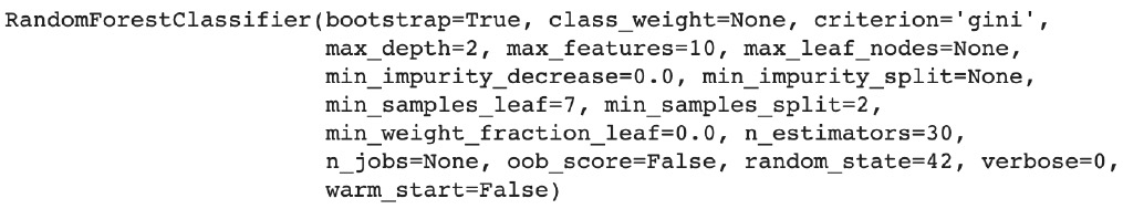
Figure 4.39: Logs of RandomForest
- Make predictions on the training and testing sets with .predict() and save the results into two new variables called train_preds and test_preds:
train_preds = rf_model.predict(X_train)
test_preds = rf_model.predict(X_test)
- Calculate the accuracy scores for the training and testing sets and save the results in two new variables called train_acc and test_acc:
train_acc = accuracy_score(y_train, train_preds)
test_acc = accuracy_score(y_test, test_preds)
- Print the accuracy scores: train_acc and test_acc:
print(train_acc)
print(test_acc)
You should get the following output:

Figure 4.40: Accuracy scores for the training and testing sets
- Instantiate another RandomForestClassifier with random_state=42, n_estimators=30, max_depth=2, min_samples_leaf=7, and max_features=0.2, and then fit the model with the training set:
rf_model2 = RandomForestClassifier(random_state=42,
n_estimators=30,
max_depth=2,
min_samples_leaf=7,
max_features=0.2)
rf_model2.fit(X_train, y_train)
You should get the following output:

Figure 4.41: Logs of RandomForest with max_features = 0.2
- Make predictions on the training and testing sets with .predict() and save the results into two new variables called train_preds2 and test_preds2:
train_preds2 = rf_model2.predict(X_train)
test_preds2 = rf_model2.predict(X_test)
- Calculate the accuracy score for the training and testing sets and save the results in two new variables called train_acc2 and test_acc2:
train_acc2 = accuracy_score(y_train, train_preds2)
test_acc2 = accuracy_score(y_test, test_preds2)
- Print the accuracy scores: train_acc and test_acc:
print(train_acc2)
print(test_acc2)
You should get the following output:

Figure 4.42: Accuracy scores for the training and testing sets
The values 10 and 0.2, which we tried in this exercise for the max_features hyperparameter, did improve the accuracy of the training set but not the testing set. With these values, the model starts to overfit again. The optimal value for max_features is the default value (sqrt) for this dataset. In the end, we succeeded in building a model with a 0.8 accuracy score that is not overfitting. This is a pretty good result given the fact the dataset wasn't big: we got only 6 features and 41759 observations.
Note
To access the source code for this specific section, please refer to https://packt.live/3g8nTk7.
You can also run this example online at https://packt.live/324quGv.
Activity 4.01: Train a Random Forest Classifier on the ISOLET Dataset
You are working for a technology company and they are planning to launch a new voice assistant product. You have been tasked with building a classification model that will recognize the letters spelled out by a user based on the signal frequencies captured. Each sound can be captured and represented as a signal composed of multiple frequencies.
Note
This activity uses the ISOLET dataset, taken from the UCI Machine Learning Repository from the following link: https://packt.live/2QFOawy.
The CSV version of this dataset can be found here: https://packt.live/36DWHpi.
The following steps will help you to complete this activity:
- Download and load the dataset using .read_csv() from pandas.
- Extract the response variable using .pop() from pandas.
- Split the dataset into training and test sets using train_test_split() from sklearn.model_selection.
- Create a function that will instantiate and fit a RandomForestClassifier using .fit() from sklearn.ensemble.
- Create a function that will predict the outcome for the training and testing sets using .predict().
- Create a function that will print the accuracy score for the training and testing sets using accuracy_score() from sklearn.metrics.
- Train and get the accuracy score for a range of different hyperparameters. Here are some options you can try:
- n_estimators = 20 and 50
- max_depth = 5 and 10
- min_samples_leaf = 10 and 50
- max_features = 0.5 and 0.3
- Select the best hyperparameter value.
These are the accuracy scores for the best model we trained:

Figure 4.43: Accuracy scores for the Random Forest classifier
Note
The solution to the activity can be found here: https://packt.live/2GbJloz.
Summary
We have finally reached the end of this chapter on multiclass classification with Random Forest. We learned that multiclass classification is an extension of binary classification: instead of predicting only two classes, target variables can have many more values. We saw how we can train a Random Forest model in just a few lines of code and assess its performance by calculating the accuracy score for the training and testing sets. Finally, we learned how to tune some of its most important hyperparameters: n_estimators, max_depth, min_samples_leaf, and max_features. We also saw how their values can have a significant impact on the predictive power of a model but also on its ability to generalize to unseen data.
In real projects, it is extremely important to choose a valid testing set. This is your final proxy before putting a model into production so you really want it to reflect the types of data you think it will receive in the future. For instance, if your dataset has a date field, you can use the last few weeks or months as your testing set and everything before that date as the training set. If you don't choose the testing set properly, you may end up with a very good model that seems to not overfit but once in production, it will generate incorrect results. The problem doesn't come from the model but from the fact the testing set was chosen poorly.
In some projects, you may see that the dataset is split into three different sets: training, validation, and testing. The validation set can be used to tune the hyperparameters and once you are confident enough, you can test your model on the testing set. As mentioned earlier, we don't want the model to see too much of the testing set but hyperparameter tuning requires you to run a model several times until you find the optimal values. This is the reason why most data scientists create a validation set for this purpose and only use the testing set a handful of times. This will be explained in more depth in Chapter 7, The Generalization of Machine Learning Models.
In the next chapter, you will be introduced to unsupervised learning and will learn how to build a clustering model with the k-means algorithm.