Overview
This chapter will teach you how to make use of the data you have to train better models by either splitting your data if it is sufficient or making use of cross-validation if it is not. By the end of this chapter, you will know how to split your data into training, validation, and test datasets. You will be able to identify the ratio in which data has to be split and also consider certain features while splitting. You will also be able to implement cross-validation to use limited data for testing and use regularization to reduce overfitting in models.
Introduction
In the previous chapter, you learned about model assessment using various metrics such as R2 score, MAE, and accuracy. These metrics help you decide which models to keep and which ones to discard. In this chapter, you will learn some more techniques for training better models.
Generalization deals with getting your models to perform well enough on data points that they have not encountered in the past (that is, during training). We will address two specific areas:
- How to make use of as much of your data as possible to train a model
- How to reduce overfitting in a model
Overfitting
A model is said to overfit the training data when it generates a hypothesis that accounts for every example. What this means is that it correctly predicts the outcome of every example. The problem with this scenario is that the model equation becomes extremely complex, and such models have been observed to be incapable of correctly predicting new observations.
Overfitting occurs when a model has been over-engineered. Two of the ways in which this could occur are:
- The model is trained on too many features.
- The model is trained for too long.
We'll discuss each of these two points in the following sections.
Training on Too Many Features
When a model trains on too many features, the hypothesis becomes extremely complicated. Consider a case in which you have one column of features and you need to generate a hypothesis. This would be a simple linear equation, as shown here:

Figure 7.1: Equation for a hypothesis for a line
Now, consider a case in which you have two columns, and in which you cross the columns by multiplying them. The hypothesis becomes the following:

Figure 7.2: Equation for a hypothesis for a curve
While the first equation yields a line, the second equation yields a curve, because it is now a quadratic equation. But the same two features could become even more complicated depending on how you engineer your features. Consider the following equation:

Figure 7.3: Cubic equation for a hypothesis
The same set of features has now given rise to a cubic equation. This equation will have the property of having a large number of weights, for example:
- The simple linear equation has one weight and one bias.
- The quadratic equation has three weights and one bias.
- The cubic equation has five weights and one bias.
One solution to overfitting as a result of too many features is to eliminate certain features. The technique for this is called lasso regression.
A second solution to overfitting as a result of too many features is to provide more data to the model. This might not always be a feasible option, but where possible, it is always a good idea to do so.
Training for Too Long
The model starts training by initializing the vector of weights such that all values are equal to zero. During training, the weights are updated according to the gradient update rule. This systematically adds or subtracts a small value to each weight. As training progresses, the magnitude of the weights increases. If the model trains for too long, these model weights become too large.
The solution to overfitting as a result of large weights is to reduce the magnitude of the weights to as close to zero as possible. The technique for this is called ridge regression.
Underfitting
Consider an alternative situation in which the data has 10 features, but you only make use of 1 feature. Your model hypothesis would still be the following:

Figure 7.4: Equation for a hypothesis for a line
However, that is the equation of a straight line, but your model is probably ignoring a lot of information. The model is over-simplified and is said to underfit the data.
The solution to underfitting is to provide the model with more features, or conversely, less data to train on; but more features is the better approach.
Data
In the world of machine learning, the data that you have is not used in its entirety to train your model. Instead, you need to separate your data into three sets, as mentioned here:
- A training dataset, which is used to train your model and measure the training loss.
- An evaluation or validation dataset, which you use to measure the validation loss of the model to see whether the validation loss continues to reduce as well as the training loss.
- A test dataset for final testing to see how well the model performs before you put it into production.
The Ratio for Dataset Splits
The evaluation dataset is set aside from your entire training data and is never used for training. There are various schools of thought around the particular ratio that is set aside for evaluation, but it generally ranges from a high of 30% to a low of 10%. This evaluation dataset is normally further split into a validation dataset that is used during training and a test dataset that is used at the end for a sanity check. If you are using 10% for evaluation, you might set 5% aside for validation and the remaining 5% for testing. If using 30%, you might set 20% aside for validation and 10% for testing.
To summarize, you might split your data into 70% for training, 20% for validation, and 10% for testing, or you could split your data into 80% for training, 15% for validation, and 5% for test. Or, finally, you could split your data into 90% for training, 5% for validation, and 5% for testing.
The choice of what ratio to use is dependent on the amount of data that you have. If you are working with 100,000 records, for example, then 20% validation would give you 20,000 records. However, if you were working with 100,000,000 records, then 5% would give you 5 million records for validation, which would be more than sufficient.
Creating Dataset Splits
At a very basic level, splitting your data involves random sampling. Let's say you have 10 items in a bowl. To get 30% of the items, you would reach in and take any 3 items at random.
In the same way, because you are writing code, you could do the following:
- Create a Python list.
- Place 10 numbers in the list.
- Generate 3 non-repeating random whole numbers from 0 to 9.
- Pick items whose indices correspond to the random numbers previously generated.

Figure 7.5: Visualization of data splitting
This is something you will only do once for a particular dataset. You might write a function for it. If it is something that you need to do repeatedly and you also need to handle advanced functionality, you might want to write a class for it.
sklearn has a class called train_test_split, which provides the functionality for splitting data. It is available as sklearn.model_selection.train_test_split. This function will let you split a DataFrame into two parts.
Have a look at the following exercise on importing and splitting data.
Exercise 7.01: Importing and Splitting Data
The goal of this exercise is to import data from a repository and to split it into a training and an evaluation set.
We will be using the Cars dataset from the UCI Machine Learning Repository.
Note
You can find the dataset here: https://packt.live/2RE5rWi
The dataset can also be found on our GitHub, here: https://packt.live/36cvyc4
You will be using this dataset throughout the exercises in this chapter.
This dataset is about the cost of owning cars with certain attributes. The abstract from the website states: "Derived from simple hierarchical decision model, this database may be useful for testing constructive induction and structure discovery methods." Here are some of the key attributes of this dataset:
CAR car acceptability
. PRICE overall price
. . buying buying price
. . maint price of the maintenance
. TECH technical characteristics
. . COMFORT comfort
. . . doors number of doors
. . . persons capacity in terms of persons to carry
. . . lug_boot the size of luggage boot
. . safety estimated safety of the car
The following steps will help you complete the exercise:
- Open a new Colab notebook file.
- Import the necessary libraries:
# import libraries
import pandas as pd
from sklearn.model_selection import train_test_split
In this step, you have imported pandas and aliased it as pd. As you know, pandas is required to read in the file. You also import train_test_split from sklearn.model_selection to split the data into two parts.
- Before reading the file into your notebook, open and inspect the file (car.data) with an editor. You should see an output similar to the following:

Figure 7.6: Car data
You will notice from the preceding screenshot that the file doesn't have a first row containing the headers.
- Create a Python list to hold the headers for the data:
# data doesn't have headers, so let's create headers
_headers = ['buying', 'maint', 'doors', 'persons',
'lug_boot', 'safety', 'car']
- Now, import the data as shown in the following code snippet:
# read in cars dataset
df = pd.read_csv('https://raw.githubusercontent.com/'
'PacktWorkshops/The-Data-Science-Workshop/'
'master/Chapter07/Dataset/car.data',
names=_headers, index_col=None)
You then proceed to import the data into a variable called df by using pd.read_csv. You specify the location of the data file, as well as the list of column headers. You also specify that the data does not have a column index.
- Show the top five records:
df.info()
In order to get information about the columns in the data as well as the number of records, you make use of the info() method. You should get an output similar to the following:

Figure 7.7: The top five records of the DataFrame
The RangeIndex value shows the number of records, which is 1728.
- Now, you need to split the data contained in df into a training dataset and an evaluation dataset:
#split the data into 80% for training and 20% for evaluation
training_df, eval_df = train_test_split(df, train_size=0.8,
random_state=0)
In this step, you make use of train_test_split to create two new DataFrames called training_df and eval_df.
You specify a value of 0.8 for train_size so that 80% of the data is assigned to training_df.
random_state ensures that your experiments are reproducible. Without random_state, the data is split differently every time using a different random number. With random_state, the data is split the same way every time. We will be studying random_state in depth in the next chapter.
- Check the information of training_df:
training_df.info()
In this step, you make use of .info() to get the details of training_df. This will print out the column names as well as the number of records.
You should get an output similar to the following:
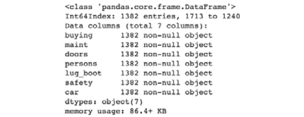
Figure 7.8: Information on training_df
You should observe that the column names match those in df, but you should have 80% of the records that you did in df, which is 1382 out of 1728.
- Check the information on eval_df:
eval_df.info()
In this step, you print out the information about eval_df. This will give you the column names and the number of records. The output should be similar to the following:

Figure 7.9: Information on eval_df
Note
To access the source code for this specific section, please refer to https://packt.live/3294avL.
You can also run this example online at https://packt.live/2E8FHhT.
Now you know how to split your data. Whenever you split your data, the records are going to be exactly the same. You could repeat the exercise a number of times and notice the range of entries in the index for eval_df.
The implication of this is that you cannot repeat your experiments. If you run the same code, you will get different results every time. Also, if you share your code with your colleagues, they will get different results. This is because the compiler makes use of random numbers.
These random numbers are not actually random but make use of something called a pseudo-random number generator. The generator has a pre-determined set of random numbers that it uses, and as a result, you can specify a random state that will cause it to use a particular set of random numbers.
Random State
The key to reproducing the same results is called random state. You simply specify a number, and whenever that number is used, the same results will be produced. This works because computers don't have an actual random number generator. Instead, they have a pseudo-random number generator. This means that you can generate the same sequence of random numbers if you set a random state.
Consider the following figure as an example. The columns are your random states. If you pick 0 as the random state, the following numbers will be generated: 41, 52, 38, 56…
However, if you pick 1 as the random state, a different set of numbers will be generated, and so on.

Figure 7.10: Numbers generated using random state
In the previous exercise, you set the random state to 0 so that the experiment was repeatable.
Exercise 7.02: Setting a Random State When Splitting Data
The goal of this exercise is to have a reproducible way of splitting the data that you imported in Exercise 7.01, Importing and Splitting Data.
Note
We going to refactor the code from the previous exercise. Hence, if you are using a new Colab notebook then make sure you copy the code from the previous exercise. Alternatively, you can make a copy of the notebook used in Exercise 7.01 and use the revised the code as suggested in the following steps.
The following steps will help you complete the exercise:
- Continue from the previous Exercise 7.01 notebook.
- Set the random state as 1 and split the data:
"""
split the data into 80% for training and 20% for evaluation
using a random state
"""
training_df, eval_df = train_test_split(df, train_size=0.8,
random_state=1)
In this step, you specify a random_state value of 1 to the train_test_split function.
- Now, view the top five records in training_df:
#view the head of training_eval
training_df.head()
In this step, you print out the first five records in training_df.
The output should be similar to the following:

Figure 7.11: The top five rows for the training evaluation set
- View the top five records in eval_df:
#view the top of eval_df
eval_df.head()
In this step, you print out the first five records in eval_df.
The output should be similar to the following:
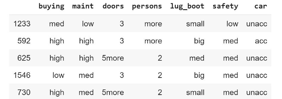
Figure 7.12: The top five rows of eval_df
Note
To access the source code for this specific section, please refer to https://packt.live/2Q6Jb7e.
You can also run this example online at https://packt.live/2EjFvMp.
The goal of this exercise is to get reproducible splits. If you run the code, you will get the same records in both training_df and eval_df. You may proceed to run that code a few times on every system and verify that you get the same records in both datasets.
Whenever you change random_state, you will get a different set of training and validation data.
But how do you find the best dataset split to train your model? When you don't have a lot of data, the recommended approach is to make use of all of your data.
But how do you retain validation data if you make use of all of your data?
The answer is to split the data into a number of parts. This approach is called cross-validation, which we will be looking at in the next section.
Cross-Validation
Consider an example where you split your data into five parts of 20% each. You would then make use of four parts for training and one part for evaluation. Because you have five parts, you can make use of the data five times, each time using one part for validation and the remaining data for training.

Figure 7.13: Cross-validation
Cross-validation is an approach to splitting your data where you make multiple splits and then make use of some of them for training and the rest for validation. You then make use of all of the combinations of data to train multiple models.
This approach is called n-fold cross-validation or k-fold cross-validation.
Note
For more information on k-fold cross-validation, refer to https://packt.live/36eXyfi.
KFold
The KFold class in sklearn.model_selection returns a generator that provides a tuple with two indices, one for training and another for testing or validation. A generator function lets you declare a function that behaves like an iterator, thus letting you use it in a loop.
Exercise 7.03: Creating a Five-Fold Cross-Validation Dataset
The goal of this exercise is to create a five-fold cross-validation dataset from the data that you imported in Exercise 7.01, Importing and Splitting Data.
Note
If you are using a new Colab notebook then make sure you copy the code from Exercise 7.01, Importing and Splitting Data. Alternatively, you can make a copy of the notebook used in Exercise 7.01 and then use the code as suggested in the following steps.
The following steps will help you complete the exercise:
- Continue from the notebook file of Exercise 7.01.
- Import all the necessary libraries:
from sklearn.model_selection import KFold
In this step, you import KFold from sklearn.model_selection.
- Now create an instance of the class:
_kf = KFold(n_splits=5)
In this step, you create an instance of KFold and assign it to a variable called _kf. You specify a value of 5 for the n_splits parameter so that it splits the dataset into five parts.
- Now split the data as shown in the following code snippet:
indices = _kf.split(df)
In this step, you call the split method, which is .split() on _kf. The result is stored in a variable called indices.
- Find out what data type indices has:
print(type(indices))
In this step, you inspect the call to split the output returns.
The output should be a generator, as seen in the following output:

Figure 7.14: Data type for indices
- Get the first set of indices:
#first set
train_indices, val_indices = next(indices)
In this step, you make use of the next() Python function on the generator function. Using next() is the way that you get a generator to return results to you. You asked for five splits, so you can call next() five times on this particular generator. Calling next() a sixth time will cause the Python runtime to raise an exception.
The call to next() yields a tuple. In this case, it is a pair of indices. The first one contains your training indices and the second one contains your validation indices. You assign these to train_indices and val_indices.
- Create a training dataset as shown in the following code snippet:
train_df = df.drop(val_indices)
train_df.info()
In this step, you create a new DataFrame called train_df by dropping the validation indices from df, the DataFrame that contains all of the data. This is a subtractive operation similar to what is done in set theory. The df set is a union of train and val. Once you know what val is, you can work backward to determine train by subtracting val from df. If you consider df to be a set called A, val to be a set called B, and train to be a set called C, then the following holds true:

Figure 7.15: Dataframe A
Similarly, set C can be the difference between set A and set B, as depicted in the following:

Figure 7.16: Dataframe C
The way to accomplish this with a pandas DataFrame is to drop the rows with the indices of the elements of B from A, which is what you see in the preceding code snippet.
You can see the result of this by calling the info() method on the new DataFrame.
The result of that call should be similar to the following screenshot:

Figure 7.17: Information on the new dataframe
- Create a validation dataset:
val_df = df.drop(train_indices)
val_df.info()
In this step, you create the val_df validation dataset by dropping the training indices from the df DataFrame. Again, you can see the details of this new DataFrame by calling the info() method.
The output should be similar to the following:

Figure 7.18: Information for the validation dataset
Note
To access the source code for this specific section, please refer to https://packt.live/3kRRaDf.
You can also run this example online at https://packt.live/3kTNPnf.
You could program all of the preceding in a loop so that you do not need to manually make a call to next() five times. This is what we will be doing in the next exercise.
Exercise 7.04: Creating a Five-Fold Cross-Validation Dataset Using a Loop for Calls
The goal of this exercise is to create a five-fold cross-validation dataset from the data that you imported in Exercise 7.01, Importing and Splitting Data. You will make use of a loop for calls to the generator function.
Note
If you are using a new Colab notebook then make sure you copy the code from Exercise 7.01, Importing and Splitting Data. Alternatively, you can make a copy of the notebook used in Exercise 7.01 and then use the code as suggested in the following steps. The link to notebook for this exercise can be found here: https://packt.live/3g83AmU
The following steps will help you complete this exercise:
- Open a new Colab notebook and repeat the steps you used to import data in Exercise 7.01, Importing and Splitting Data.
- Define the number of splits you would like:
from sklearn.model_selection import KFold
#define number of splits
n_splits = 5
In this step, you set the number of splits to 5. You store this in a variable called n_splits.
- Create an instance of Kfold:
#create an instance of KFold
_kf = KFold(n_splits=n_splits)
In this step, you create an instance of Kfold. You assign this instance to a variable called _kf.
- Generate the split indices:
#create splits as _indices
_indices = _kf.split(df)
In this step, you call the split() method on _kf, which is the instance of KFold that you defined earlier. You provide df as a parameter so that the splits are performed on the data contained in the DataFrame called df. The resulting generator is stored as _indices.
- Create two Python lists:
_t, _v = [], []
In this step, you create two Python lists. The first is called _t and holds the training DataFrames, and the second is called _v and holds the validation DataFrames.
- Iterate over the generator and create DataFrames called train_idx, val_idx, _train_df and _val_df:
#iterate over _indices
for i in range(n_splits):
train_idx, val_idx = next(_indices)
_train_df = df.drop(val_idx)
_t.append(_train_df)
_val_df = df.drop(train_idx)
_v.append(_val_df)
In this step, you create a loop using range to determine the number of iterations. You specify the number of iterations by providing n_splits as a parameter to range(). On every iteration, you execute next() on the _indices generator and store the results in train_idx and val_idx. You then proceed to create _train_df by dropping the validation indices, val_idx, from df. You also create _val_df by dropping the training indices from df.
- Iterate over the training list:
for d in _t:
print(d.info())
In this step, you verify that the compiler created the DataFrames. You do this by iterating over the list and using the .info() method to print out the details of each element. The output is similar to the following screenshot, which is incomplete due to the size of the output. Each element in the list is a DataFrame with 1,382 entries:

Figure 7.19: Iterating over the training list
Note
The preceding output is a truncated version of the actual output.
- Iterate over the validation list:
for d in _v:
print(d.info())
In this step, you iterate over the validation list and make use of .info() to print out the details of each element. The output is similar to the following screenshot, which is incomplete due to the size. Each element is a DataFrame with 346 entries:
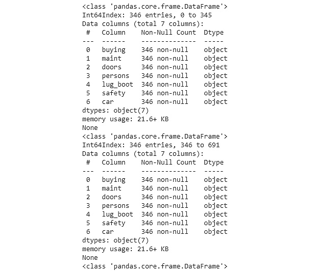
Figure 7.20: Iterating over the validation list
Note
The preceding output is a truncated version of the actual output.
To access the source code for this specific section, please refer to https://packt.live/3g83AmU.
You can also run this example online at https://packt.live/3iXwEPR.
In this exercise, you have learned how to use a loop for k-fold cross-validation to extract training and validation datasets. You can make use of these datasets to train and evaluate multiple models.
The essence of creating cross-validation datasets is that you can train and evaluate multiple models. What if you didn't have to train those models in a loop?
The good news is that you can avoid training multiple models in a loop because if you did that, you would need arrays to track lots of metrics.
cross_val_score
The cross_val_score() function is available in sklearn.model_selection. Up until this point, you have learned how to create cross-validation datasets in a loop. If you made use of that approach, you would need to keep track of all of the models that you are training and evaluating inside of that loop.
cross_val_score takes care of the following:
- Creating cross-validation datasets
- Training models by fitting them to the training data
- Evaluating the models on the validation data
- Returning a list of the R2 score of each model that is trained
For all of the preceding actions to happen, you will need to provide the following inputs:
- An instance of an estimator (for example, LinearRegression)
- The original dataset
- The number of splits to create (which is also the number of models that will be trained and evaluated)
Exercise 7.05: Getting the Scores from Five-Fold Cross-Validation
The goal of this exercise is to create a five-fold cross-validation dataset from the data that you imported in Exercise 7.01, Importing and Splitting Data. You will then use cross_val_score to get the scores of models trained on those datasets.
Note
If you are using a new Colab notebook then make sure you copy the code from Exercise 7.01, Importing and Splitting Data. Alternatively, you can make a copy of the notebook used in Exercise 7.01 and then use the revised code as suggested in the following steps. The link to notebook for this exercise can be found here: https://packt.live/2DWTkAY.
The following steps will help you complete the exercise:
- Open a new Colab notebook and repeat steps 1-6 that you took to import data in Exercise 7.01, Importing and Splitting Data.
- Encode the categorical variables in the dataset:
# encode categorical variables
_df = pd.get_dummies(df, columns=['buying', 'maint', 'doors',
'persons', 'lug_boot',
'safety'])
_df.head()
In this step, you make use of pd.get_dummies() to convert categorical variables into an encoding. You store the result in a new DataFrame variable called _df. You then proceed to take a look at the first five records.
The result should look similar to the following:

Figure 7.21: Encoding categorical variables
- Split the data into features and labels:
# separate features and labels DataFrames
features = _df.drop(['car'], axis=1).values
labels = _df[['car']].values
In this step, you create a features DataFrame by dropping car from _df. You also create labels by selecting only car in a new DataFrame. Here, a feature and a label are similar in the Cars dataset.
- Create an instance of the LogisticRegression class to be used later:
from sklearn.linear_model import LogisticRegression
# create an instance of LogisticRegression
_lr = LogisticRegression()
In this step, you import LogisticRegression from sklearn.linear_model. We use LogisticRegression because it lets us create a classification model, as you learned in Chapter 3, Binary Classification. You then proceed to create an instance and store it as _lr.
- Import the cross_val_score function:
from sklearn.model_selection import cross_val_score
In this step now, you import cross_val_score, which you will make use of to compute the scores of the models.
- Compute the cross-validation scores:
_scores = cross_val_score(_lr, features, labels, cv=5)
In this step, you the compute cross-validation scores and store the result in a Python list, which you call _scores. You do this using cross_cal_score. The function requires the following four parameters: the model to make use of (in our case, it's called _lr); the features of the dataset; the labels of the dataset; and the number of cross-validation splits to create (five, in our case).
- Now, display the scores as shown in the following code snippet:
print(_scores)
In this step, you display the scores using print().
The output should look similar to the following:

Figure 7.22: Printing the cross-validation scores
Note
You may get slightly different outputs but the best score should belong to second split.
To access the source code for this specific section, please refer to https://packt.live/2DWTkAY.
You can also run this example online at https://packt.live/34d5aS8.
In the preceding output, you see that the Python list stored in variable _scores contains five results. Each result is the R2 score of a LogisticRegression model. As mentioned before the exercise, the data will be split into five sets, and each combination of the five sets will be used to train and evaluate a model, after which the R2 score is computed.
You should observe from the preceding example that the same model trained on five different datasets yields different scores. This implies the importance of your data as well as how it is split.
By completing this exercise, we see that the best score is 0.832, which belongs to the second split. This is our conclusion here.
You have seen that cross-validation yields different models.
But how do you get the best model to work with? There are some models or estimators with in-built cross-validation. Let's explain those.
Understanding Estimators That Implement CV
The goal of using cross-validation is to find the best performing model using the data that you have. The process for this is:
- Split the data using something like Kfold().
- Iterate over the number of splits and create an estimator.
- Train and evaluate each estimator.
- Pick the estimator with the best metrics to use. You have already seen various approaches to doing that.
Cross-validation is a popular technique, so estimators exist for cross-validation. For example, LogisticRegressionCV exists as a class that implements cross-validation inside LogisticRegression. When you make use of LogisticRegressionCV, it returns an instance of LogisticRegression. The instance it returns is the best performing instance.
When you create an instance of LogisticRegressionCV, you will need to specify the number of cv parts that you want. For example, if you set cv to 3, LogisticRegressionCV will train three instances of LogisticRegression and then evaluate them and return the best performing instance.
You do not have to make use of LogisticRegressionCV. You can continue to make use of LogisticRegression with Kfold and iterations. LogisticRegressionCV simply exists as a convenience.
In a similar manner, LinearRegressionCV exists as a convenient way of implementing cross-validation using LinearRegression.
So, just to be clear, you do not have to use convenience methods such as LogisticRegressionCV. Also, they are not a replacement for their primary implementations, such as LogisticRegression. Instead, you make use of the convenience methods when you need to implement cross-validation but would like to cut out the four preceding steps.
LogisticRegressionCV
LogisticRegressionCV is a class that implements cross-validation inside it. This class will train multiple LogisticRegression models and return the best one.
Exercise 7.06: Training a Logistic Regression Model Using Cross-Validation
The goal of this exercise is to train a logistic regression model using cross-validation and get the optimal R2 result. We will be making use of the Cars dataset that you worked with previously.
The following steps will help you complete the exercise:
- Open a new Colab notebook.
- Import the necessary libraries:
# import libraries
import pandas as pd
from sklearn.model_selection import train_test_split
In this step, you import pandas and alias it as pd. You will make use of pandas to read in the file you will be working with.
- Create headers for the data:
# data doesn't have headers, so let's create headers
_headers = ['buying', 'maint', 'doors', 'persons',
'lug_boot', 'safety', 'car']
In this step, you start by creating a Python list to hold the headers column for the file you will be working with. You store this list as _headers.
- Read the data:
# read in cars dataset
df = pd.read_csv('https://raw.githubusercontent.com/'
'PacktWorkshops/The-Data-Science-Workshop/'
'master/Chapter07/Dataset/car.data',
names=_headers, index_col=None)
You then proceed to read in the file and store it as df. This is a DataFrame.
- Print out the top five records:
df.info()
Finally, you look at the summary of the DataFrame using .info().
The output looks similar to the following:
Figure 7.23: The top five records of the dataframe
- Encode the categorical variables as shown in the following code snippet:
# encode categorical variables
_df = pd.get_dummies(df, columns=['buying', 'maint', 'doors',
'persons', 'lug_boot',
'safety'])
_df.head()
In this step, you convert categorical variables into encodings using the get_dummies() method from pandas. You supply the original DataFrame as a parameter and also specify the columns you would like to encode.
Finally, you take a peek at the top five rows. The output looks similar to the following:
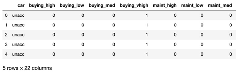
Figure 7.24: Encoding categorical variables
- Split the DataFrame into features and labels:
# separate features and labels DataFrames
features = _df.drop(['car'], axis=1).values
labels = _df[['car']].values
In this step, you create two NumPy arrays. The first, called features, contains the independent variables. The second, called labels, contains the values that the model learns to predict. These are also called targets.
- Import logistic regression with cross-validation:
from sklearn.linear_model import LogisticRegressionCV
In this step, you import the LogisticRegressionCV class.
- Instantiate LogisticRegressionCV as shown in the following code snippet:
model = LogisticRegressionCV(max_iter=2000, multi_class='auto',
cv=5)
In this step, you create an instance of LogisticRegressionCV. You specify the following parameters:
max_iter : You set this to 2000 so that the trainer continues training for 2000 iterations to find better weights.
multi_class: You set this to auto so that the model automatically detects that your data has more than two classes.
cv: You set this to 5, which is the number of cross-validation sets you would like to train on.
- Now fit the model:
model.fit(features, labels.ravel())
In this step, you train the model. You pass in features and labels. Because labels is a 2D array, you make use of ravel() to convert it into a 1D array or vector.
The interpreter produces an output similar to the following:

Figure 7.25: Fitting the model
In the preceding output, you see that the model fits the training data. The output shows you the parameters that were used in training, so you are not taken by surprise. Notice, for example, that max_iter is 2000, which is the value that you set. Other parameters you didn't set make use of default values, which you can find out more about from the documentation.
- Evaluate the training R2:
print(model.score(features, labels.ravel()))
In this step, we make use of the training dataset to compute the R2 score. While we didn't set aside a specific validation dataset, it is important to note that the model only saw 80% of our training data, so it still has new data to work with for this evaluation.
The output looks similar to the following:

Figure 7.26: Computing the R2 score
Note
To access the source code for this specific section, please refer to https://packt.live/34eD1du.
You can also run this example online at https://packt.live/2Yey40k.
In the preceding output, you see that the final model has an R2 score of 0.95, which is a good score.
At this point, you should see a much better R2 score than you have previously encountered.
What if you were working with other types of models that don't have cross-validation built into them? Can you make use of cross-validation to train models and find the best one? Let's find out.
Hyperparameter Tuning with GridSearchCV
GridSearchCV will take a model and parameters and train one model for each permutation of the parameters. At the end of the training, it will provide access to the parameters and the model scores. This is called hyperparameter tuning and you will be looking at this in much more depth in Chapter 8, Hyperparameter Tuning.
The usual practice is to make use of a small training set to find the optimal parameters using hyperparameter tuning and then to train a final model with all of the data.
Before the next exercise, let's take a brief look at decision trees, which are a type of model or estimator.
Decision Trees
A decision tree works by generating a separating hyperplane or a threshold for the features in data. It does this by considering every feature and finding the correlation between the spread of the values in that feature and the label that you are trying to predict.
Consider the following data about balloons. The label you need to predict is called inflated. This dataset is used for predicting whether the balloon is inflated or deflated given the features. The features are:
- color
- size
- act
- age
The following table displays the distribution of features:

Figure 7.27: Tabular data for balloon features
Now consider the following charts, which are visualized depending on the spread of the features against the label:
- If you consider the Color feature, the values are PURPLE and YELLOW, but the number of observations is the same, so you can't infer whether the balloon is inflated or not based on the color, as you can see in the following figure:

Figure 7.28: Barplot for the color feature
- The Size feature has two values: LARGE and SMALL. These are equally spread, so we can't infer whether the balloon is inflated or not based on the color, as you can see in the following figure:

Figure 7.29: Barplot for the size feature
- The Act feature has two values: DIP and STRETCH. You can see from the chart that the majority of the STRETCH values are inflated. If you had to make a guess, you could easily say that if Act is STRETCH, then the balloon is inflated. Consider the following figure:

Figure 7.30: Barplot for the act feature
- Finally, the Age feature also has two values: ADULT and CHILD. It's also visible from the chart that the ADULT value constitutes the majority of inflated balloons:

Figure 7.31: Barplot for the age feature
The two features that are useful to the decision tree are Act and Age. The tree could start by considering whether Act is STRETCH. If it is, the prediction will be true. This tree would look like the following figure:

Figure 7.32: Decision tree with depth=1
The left side evaluates to the condition being false, and the right side evaluates to the condition being true. This tree has a depth of 1. F means that the prediction is false, and T means that the prediction is true.
To get better results, the decision tree could introduce a second level. The second level would utilize the Age feature and evaluate whether the value is ADULT. It would look like the following figure:

Figure 7.33: Decision tree with depth=2
This tree has a depth of 2. At the first level, it predicts true if Act is STRETCH. If Act is not STRETCH, it checks whether Age is ADULT. If it is, it predicts true, otherwise, it predicts false.
The decision tree can have as many levels as you like but starts to overfit at a certain point. As with everything in data science, the optimal depth depends on the data and is a hyperparameter, meaning you need to try different values to find the optimal one.
In the following exercise, we will be making use of grid search with cross-validation to find the best parameters for a decision tree estimator.
Exercise 7.07: Using Grid Search with Cross-Validation to Find the Best Parameters for a Model
The goal of this exercise is to make use of grid search to find the best parameters for a DecisionTree classifier. We will be making use of the Cars dataset that you worked with previously.
The following steps will help you complete the exercise:
- Open a Colab notebook file.
- Import pandas:
import pandas as pd
In this step, you import pandas. You alias it as pd. Pandas is used to read in the data you will work with subsequently.
- Create headers:
_headers = ['buying', 'maint', 'doors', 'persons',
'lug_boot', 'safety', 'car']
- Read in the headers:
# read in cars dataset
df = pd.read_csv('https://raw.githubusercontent.com/'
'PacktWorkshops/The-Data-Science-Workshop/'
'master/Chapter07/Dataset/car.data',
names=_headers, index_col=None)
- Inspect the top five records:
df.info()
The output looks similar to the following:

Figure 7.34: The top five records of the dataframe
- Encode the categorical variables:
_df = pd.get_dummies(df, columns=['buying', 'maint', 'doors',
'persons', 'lug_boot',
'safety'])
_df.head()
In this step, you utilize .get_dummies() to convert the categorical variables into encodings. The .head() method instructs the Python interpreter to output the top five columns.
The output is similar to the following:
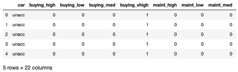
Figure 7.35: Encoding categorical variables
- Separate features and labels:
features = _df.drop(['car'], axis=1).values
labels = _df[['car']].values
In this step, you create two numpy arrays, features and labels, the first containing independent variables or predictors, and the second containing dependent variables or targets.
- Import more libraries – numpy, DecisionTreeClassifier, and GridSearchCV:
import numpy as np
from sklearn.tree import DecisionTreeClassifier
from sklearn.model_selection import GridSearchCV
In this step, you import numpy. NumPy is a numerical computation library. You alias it as np. You also import DecisionTreeClassifier, which you use to create decision trees. Finally, you import GridSearchCV, which will use cross-validation to train multiple models.
- Instantiate the decision tree:
clf = DecisionTreeClassifier()
In this step, you create an instance of DecisionTreeClassifier as clf. This instance will be used repeatedly by the grid search.
- Create parameters – max_depth:
params = {'max_depth': np.arange(1, 8)}
In this step, you create a dictionary of parameters. There are two parts to this dictionary:
The key of the dictionary is a parameter that is passed into the model. In this case, max_depth is a parameter that DecisionTreeClassifier takes.
The value is a Python list that grid search iterates over and passes to the model. In this case, we create an array that starts at 1 and ends at 7, inclusive.
- Instantiate the grid search as shown in the following code snippet:
clf_cv = GridSearchCV(clf, param_grid=params, cv=5)
In this step, you create an instance of GridSearchCV. The first parameter is the model to train. The second parameter is the parameters to search over. The third parameter is the number of cross-validation splits to create.
- Now train the models:
clf_cv.fit(features, labels)
In this step, you train the models using the features and labels. Depending on the type of model, this could take a while. Because we are using a decision tree, it trains quickly.
The output is similar to the following:

Figure 7.36: Training the model
You can learn a lot by reading the output, such as the number of cross-validation datasets created (called cv and equal to 5), the estimator used (DecisionTreeClassifier), and the parameter search space (called param_grid).
- Print the best parameter:
print("Tuned Decision Tree Parameters: {}"
.format(clf_cv.best_params_))
In this step, you print out what the best parameter is. In this case, what we were looking for was the best max_depth. The output looks like the following:

Figure 7.37: Printing the best parameter
In the preceding output, you see that the best performing model is one with a max_depth of 2.
Accessing best_params_ lets you train another model with the best-known parameters using a larger training dataset.
- Print the best R2:
print("Best score is {}".format(clf_cv.best_score_))
In this step, you print out the R2 score of the best performing model.
The output is similar to the following:
Best score is 0.7777777777777778
In the preceding output, you see that the best performing model has an R2 score of 0.778.
- Access the best model:
model = clf_cv.best_estimator_
model
In this step, you access the best model (or estimator) using best_estimator_. This will let you analyze the model, or optionally use it to make predictions and find other metrics. Instructing the Python interpreter to print the best estimator will yield an output similar to the following:

Figure 7.38: Accessing the model
In the preceding output, you see that the best model is DecisionTreeClassifier with a max_depth of 2.
Note
To access the source code for this specific section, please refer to https://packt.live/2E6TdCD.
You can also run this example online at https://packt.live/3aCg30V.
Grid search is one of the first techniques that is taught for hyperparameter tuning. However, as the search space increases in size, it quickly becomes expensive. The search space increases as you increase the parameter options because every possible combination of parameter options is considered.
Consider the case in which the model (or estimator) takes more than one parameter. The search space becomes a multiple of the number of parameters. For example, if we want to train a random forest classifier, we will need to specify the number of trees in the forest, as well as the max depth. If we specified a max depth of 1, 2, and 3, and a forest with 1,000, 2,000, and 3,000 trees, we would need to train 9 different estimators. If we added any more parameters (or hyperparameters), our search space would increase geometrically.
Hyperparameter Tuning with RandomizedSearchCV
Grid search goes over the entire search space and trains a model or estimator for every combination of parameters. Randomized search goes over only some of the combinations. This is a more optimal use of resources and still provides the benefits of hyperparameter tuning and cross-validation. You will be looking at this in depth in Chapter 8, Hyperparameter Tuning.
Have a look at the following exercise.
Exercise 7.08: Using Randomized Search for Hyperparameter Tuning
The goal of this exercise is to perform hyperparameter tuning using randomized search and cross-validation.
The following steps will help you complete this exercise:
- Open a new Colab notebook file.
- Import pandas:
import pandas as pd
In this step, you import pandas. You will make use of it in the next step.
- Create headers:
_headers = ['buying', 'maint', 'doors', 'persons',
'lug_boot', 'safety', 'car']
- Read in the data:
# read in cars dataset
df = pd.read_csv('https://raw.githubusercontent.com/'
'PacktWorkshops/The-Data-Science-Workshop/'
'master/Chapter07/Dataset/car.data',
names=_headers, index_col=None)
- Check the first five rows:
df.info()
You need to provide a Python list of column headers because the data does not contain column headers. You also inspect the DataFrame that you created.
The output is similar to the following:

Figure 7.39: The top five rows of the DataFrame
- Encode categorical variables as shown in the following code snippet:
_df = pd.get_dummies(df, columns=['buying', 'maint', 'doors',
'persons', 'lug_boot',
'safety'])
_df.head()
In this step, you find a numerical representation of text data using one-hot encoding. The operation results in a new DataFrame. You will see that the resulting data structure looks similar to the following:

Figure 7.40: Encoding categorical variables
- Separate the data into independent and dependent variables, which are the features and labels:
features = _df.drop(['car'], axis=1).values
labels = _df[['car']].values
In this step, you separate the DataFrame into two numpy arrays called features and labels. Features contains the independent variables, while labels contains the target or dependent variables.
- Import additional libraries – numpy, RandomForestClassifier, and RandomizedSearchCV:
import numpy as np
from sklearn.ensemble import RandomForestClassifier
from sklearn.model_selection import RandomizedSearchCV
In this step, you import numpy for numerical computations, RandomForestClassifier to create an ensemble of estimators, and RandomizedSearchCV to perform a randomized search with cross-validation.
- Create an instance of RandomForestClassifier:
clf = RandomForestClassifier()
In this step, you instantiate RandomForestClassifier. A random forest classifier is a voting classifier. It makes use of multiple decision trees, which are trained on different subsets of the data. The results from the trees contribute to the output of the random forest by using a voting mechanism.
- Specify the parameters:
params = {'n_estimators':[500, 1000, 2000],
'max_depth': np.arange(1, 8)}
RandomForestClassifier accepts many parameters, but we specify two: the number of trees in the forest, called n_estimators, and the depth of the nodes in each tree, called max_depth.
- Instantiate a randomized search:
clf_cv = RandomizedSearchCV(clf, param_distributions=params,
cv=5)
In this step, you specify three parameters when you instantiate the clf class, the estimator, or model to use, which is a random forest classifier, param_distributions, the parameter search space, and cv, the number of cross-validation datasets to create.
- Perform the search:
clf_cv.fit(features, labels.ravel())
In this step, you perform the search by calling fit(). This operation trains different models using the cross-validation datasets and various combinations of the hyperparameters. The output from this operation is similar to the following:

Figure 7.41: Output of the search operation
In the preceding output, you see that the randomized search will be carried out using cross-validation with five splits (cv=5). The estimator to be used is RandomForestClassifier.
- Print the best parameter combination:
print("Tuned Random Forest Parameters: {}"
.format(clf_cv.best_params_))
In this step, you print out the best hyperparameters.
The output is similar to the following:

Figure 7.42: Printing the best parameter combination
In the preceding output, you see that the best estimator is a Random Forest classifier with 1,000 trees (n_estimators=1000) and max_depth=5. You can print the best score by executing print("Best score is {}".format(clf_cv.best_score_)). For this exercise, this value is ~ 0.76.
- Inspect the best model:
model = clf_cv.best_estimator_
model
In this step, you find the best performing estimator (or model) and print out its details. The output is similar to the following:

Figure 7.43: Inspecting the model
In the preceding output, you see that the best estimator is RandomForestClassifier with n_estimators=1000 and max_depth=5.
Note
To access the source code for this specific section, please refer to https://packt.live/3aDFijn.
You can also run this example online at https://packt.live/3kWMQ5r.
In this exercise, you learned to make use of cross-validation and random search to find the best model using a combination of hyperparameters. This process is called hyperparameter tuning, in which you find the best combination of hyperparameters to use to train the model that you will put into production.
Model Regularization with Lasso Regression
As mentioned at the beginning of this chapter models can overfit training data. One reason for this is having too many features with large coefficients (also called weights). The key to solving this type of overfitting problem is reducing the magnitude of the coefficients.
You may recall that weights are optimized during model training. One method for optimizing weights is called gradient descent. The gradient update rule makes use of a differentiable loss function. Examples of differentiable loss functions are:
- Mean Absolute Error (MAE)
- Mean Squared Error (MSE)
For lasso regression, a penalty is introduced in the loss function. The technicalities of this implementation are hidden by the class. The penalty is also called a regularization parameter.
Consider the following exercise in which you over-engineer a model to introduce overfitting, and then use lasso regression to get better results.
Exercise 7.09: Fixing Model Overfitting Using Lasso Regression
The goal of this exercise is to teach you how to identify when your model starts overfitting, and to use lasso regression to fix overfitting in your model.
Note
The data you will be making use of is the Combined Cycle Power Plant Data Set from the UCI Machine Learning Repository. It contains 9568 data points collected from a Combined Cycle Power Plant. Features include temperature, pressure, humidity, and exhaust vacuum. These are used to predict the net hourly electrical energy output of the plant. See the following link: https://packt.live/2v9ohwK.
The attribute information states "Features consist of hourly average ambient variables:
- Temperature (T) in the range 1.81°C and 37.11°C,
- Ambient Pressure (AP) in the range 992.89-1033.30 millibar,
- Relative Humidity (RH) in the range 25.56% to 100.16%
- Exhaust Vacuum (V) in the range 25.36-81.56 cm Hg
- Net hourly electrical energy output (EP) 420.26-495.76 MW
The averages are taken from various sensors located around the plant that record the ambient variables every second. The variables are given without normalization."
The following steps will help you complete the exercise:
- Open a Colab notebook.
- Import the required libraries:
import pandas as pd
from sklearn.model_selection import train_test_split
from sklearn.linear_model import LinearRegression, Lasso
from sklearn.metrics import mean_squared_error
from sklearn.pipeline import Pipeline
from sklearn.preprocessing import MinMaxScaler,
PolynomialFeatures
- Read in the data:
_df = pd.read_csv('https://raw.githubusercontent.com/'
'PacktWorkshops/The-Data-Science-Workshop/'
'master/Chapter07/Dataset/ccpp.csv')
- Inspect the DataFrame:
_df.info()
The .info() method prints out a summary of the DataFrame, including the names of the columns and the number of records. The output might be similar to the following:

Figure 7.44: Inspecting the dataframe
You can see from the preceding figure that the DataFrame has 5 columns and 9,568 records. You can see that all columns contain numeric data and that the columns have the following names: AT, V, AP, RH, and PE.
- Extract features into a column called X:
X = _df.drop(['PE'], axis=1).values
- Extract labels into a column called y:
y = _df['PE'].values
- Split the data into training and evaluation sets:
train_X, eval_X, train_y, eval_y = train_test_split
(X, y, train_size=0.8,
random_state=0)
- Create an instance of a LinearRegression model:
lr_model_1 = LinearRegression()
- Fit the model on the training data:
lr_model_1.fit(train_X, train_y)
The output from this step should look similar to the following:

Figure 7.45: Fitting the model on training data
- Use the model to make predictions on the evaluation dataset:
lr_model_1_preds = lr_model_1.predict(eval_X)
- Print out the R2 score of the model:
print('lr_model_1 R2 Score: {}'
.format(lr_model_1.score(eval_X, eval_y)))
The output of this step should look similar to the following:

Figure 7.46: Printing the R2 score
You will notice that the R2 score for this model is 0.926. You will make use of this figure to compare with the next model you train. Recall that this is an evaluation metric.
- Print out the Mean Squared Error (MSE) of this model:
print('lr_model_1 MSE: {}'
.format(mean_squared_error(eval_y, lr_model_1_preds)))
The output of this step should look similar to the following:

Figure 7.47: Printing the MSE
You will notice that the MSE is 21.675. This is an evaluation metric that you will use to compare this model to subsequent models.
The first model was trained on four features. You will now train a new model on four cubed features.
- Create a list of tuples to serve as a pipeline:
steps = [('scaler', MinMaxScaler()),
('poly', PolynomialFeatures(degree=3)),
('lr', LinearRegression())]
In this step, you create a list with three tuples. The first tuple represents a scaling operation that makes use of MinMaxScaler. The second tuple represents a feature engineering step and makes use of PolynomialFeatures. The third tuple represents a LinearRegression model.
The first element of the tuple represents the name of the step, while the second element represents the class that performs a transformation or an estimator.
- Create an instance of a pipeline:
lr_model_2 = Pipeline(steps)
- Train the instance of the pipeline:
lr_model_2.fit(train_X, train_y)
The pipeline implements a .fit() method, which is also implemented in all instances of transformers and estimators. The .fit() method causes .fit_transform() to be called on transformers, and causes .fit() to be called on estimators. The output of this step is similar to the following:

Figure 7.48: Training the instance of the pipeline
You can see from the output that a pipeline was trained. You can see that the steps are made up of MinMaxScaler and PolynomialFeatures, and that the final step is made up of LinearRegression.
- Print out the R2 score of the model:
print('lr_model_2 R2 Score: {}'
.format(lr_model_2.score(eval_X, eval_y)))
The output is similar to the following:

Figure 7.49: The R2 score of the model
You can see from the preceding that the R2 score is 0.944, which is better than the R2 score of the first model, which was 0.932. You can start to observe that the metrics suggest that this model is better than the first one.
- Use the model to predict on the evaluation data:
lr_model_2_preds = lr_model_2.predict(eval_X)
- Print the MSE of the second model:
print('lr_model_2 MSE: {}'
.format(mean_squared_error(eval_y, lr_model_2_preds)))
The output is similar to the following:

Figure 7.50: The MSE of the second model
You can see from the output that the MSE of the second model is 16.27. This is less than the MSE of the first model, which is 19.73. You can safely conclude that the second model is better than the first.
- Inspect the model coefficients (also called weights):
print(lr_model_2[-1].coef_)
In this step, you will note that lr_model_2 is a pipeline. The final object in this pipeline is the model, so you make use of list addressing to access this by setting the index of the list element to -1.
Once you have the model, which is the final element in the pipeline, you make use of .coef_ to get the model coefficients. The output is similar to the following:
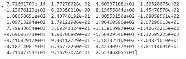
Figure 7.51: Print the model coefficients
You will note from the preceding output that the majority of the values are in the tens, some values are in the hundreds, and one value has a really small magnitude.
- Check for the number of coefficients in this model:
print(len(lr_model_2[-1].coef_))
The output for this step is similar to the following:
35
You can see from the preceding screenshot that the second model has 35 coefficients.
- Create a steps list with PolynomialFeatures of degree 10:
steps = [('scaler', MinMaxScaler()),
('poly', PolynomialFeatures(degree=10)),
('lr', LinearRegression())]
- Create a third model from the preceding steps:
lr_model_3 = Pipeline(steps)
- Fit the third model on the training data:
lr_model_3.fit(train_X, train_y)
The output from this step is similar to the following:
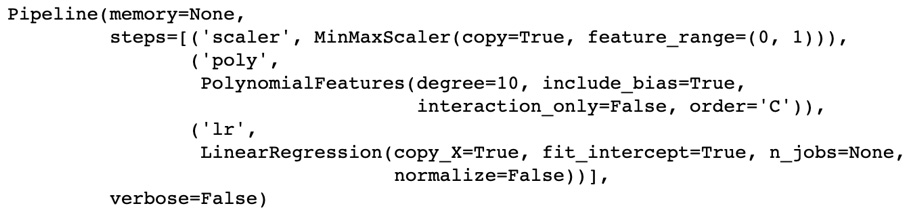
Figure 7.52: Fitting the third model on the data
You can see from the output that the pipeline makes use of PolynomialFeatures of degree 10. You are doing this in the hope of getting a better model.
- Print out the R2 score of this model:
print('lr_model_3 R2 Score: {}'
.format(lr_model_3.score(eval_X, eval_y)))
The output of this model is similar to the following:

Figure 7.53: R2 score of the model
You can see from the preceding figure that the R2 score is now 0.56. The previous model had an R2 score of 0.944. This model has an R2 score that is considerably worse than the one of the previous model, lr_model_2. This happens when your model is overfitting.
- Use lr_model_3 to predict on evaluation data:
lr_model_3_preds = lr_model_3.predict(eval_X)
- Print out the MSE for lr_model_3:
print('lr_model_3 MSE: {}'
.format(mean_squared_error(eval_y, lr_model_3_preds)))
The output for this step might be similar to the following:

Figure 7.54: The MSE of the model
You can see from the preceding figure that the MSE is also considerably worse. The MSE is 126.25, as compared to 16.27 for the previous model.
- Print out the number of coefficients (also called weights) in this model:
print(len(lr_model_3[-1].coef_))
The output might resemble the following:

Figure 7.55: Printing the number of coefficients
You can see that the model has 1,001 coefficients.
- Inspect the first 35 coefficients to get a sense of the individual magnitudes:
print(lr_model_3[-1].coef_[:35])
The output might be similar to the following:

Figure 7.56: Inspecting the first 35 coefficients
You can see from the output that the coefficients have significantly larger magnitudes than the coefficients from lr_model_2.
In the next steps, you will train a lasso regression model on the same set of features to reduce overfitting.
- Create a list of steps for the pipeline you will create later on:
steps = [('scaler', MinMaxScaler()),
('poly', PolynomialFeatures(degree=10)),
('lr', Lasso(alpha=0.01))]
You create a list of steps for the pipeline you will create. Note that the third step in this list is an instance of lasso. The parameter called alpha in the call to Lasso() is the regularization parameter. You can play around with any values from 0 to 1 to see how it affects the performance of the model that you train.
- Create an instance of a pipeline:
lasso_model = Pipeline(steps)
- Fit the pipeline on the training data:
lasso_model.fit(train_X, train_y)
The output from this operation might be similar to the following:
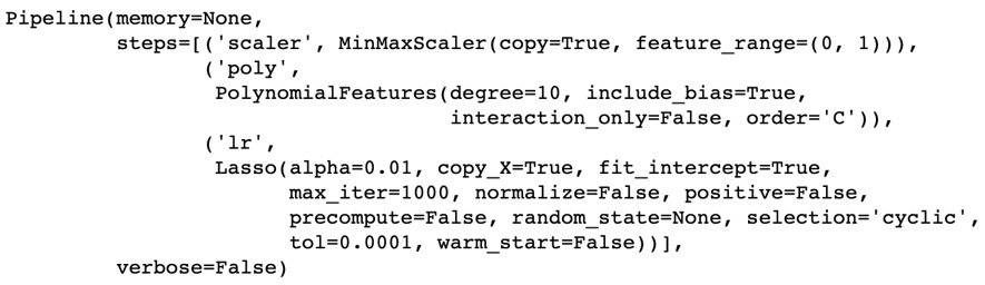
Figure 7.57: Fitting the pipeline on the training data
You can see from the output that the pipeline trained a lasso model in the final step. The regularization parameter was 0.01 and the model trained for a maximum of 1,000 iterations.
- Print the R2 score of lasso_model:
print('lasso_model R2 Score: {}'
.format(lasso_model.score(eval_X, eval_y)))
The output of this step might be similar to the following:

Figure 7.58: R2 score
You can see that the R2 score has climbed back up to 0.94, which is considerably better than the score of 0.56 that lr_model_3 had. This is already looking like a better model.
- Use lasso_model to predict on the evaluation data:
lasso_preds = lasso_model.predict(eval_X)
- Print the MSE of lasso_model:
print('lasso_model MSE: {}'
.format(mean_squared_error(eval_y, lasso_preds)))
The output might be similar to the following:

Figure 7.59: MSE of lasso model
You can see from the output that the MSE is 17.01, which is way lower than the MSE value of 126.25 that lr_model_3 had. You can safely conclude that this is a much better model.
- Print out the number of coefficients in lasso_model:
print(len(lasso_model[-1].coef_))
The output might be similar to the following:
1001
You can see that this model has 1,001 coefficients, which is the same number of coefficients that lr_model_3 had.
- Print out the values of the first 35 coefficients:
print(lasso_model[-1].coef_[:35])
The output might be similar to the following:

Figure 7.60: Printing the values of 35 coefficients
You can see from the preceding output that some of the coefficients are set to 0. This has the effect of ignoring the corresponding column of data in the input. You can also see that the remaining coefficients have magnitudes of less than 100. This goes to show that the model is no longer overfitting.
Note
To access the source code for this specific section, please refer to https://packt.live/319S6en.
You can also run this example online at https://packt.live/319AAXD.
This exercise taught you how to fix overfitting by using LassoRegression to train a new model.
In the next section, you will learn about using ridge regression to solve overfitting in a model.
Ridge Regression
You just learned about lasso regression, which introduces a penalty and tries to eliminate certain features from the data. Ridge regression takes an alternative approach by introducing a penalty that penalizes large weights. As a result, the optimization process tries to reduce the magnitude of the coefficients without completely eliminating them.
Exercise 7.10: Fixing Model Overfitting Using Ridge Regression
The goal of this exercise is to teach you how to identify when your model starts overfitting, and to use ridge regression to fix overfitting in your model.
Note
You will be using the same dataset as in Exercise 7.09, Fixing Model Overfitting Using Lasso Regression.
The following steps will help you complete the exercise:
- Open a Colab notebook.
- Import the required libraries:
import pandas as pd
from sklearn.model_selection import train_test_split
from sklearn.linear_model import LinearRegression, Ridge
from sklearn.metrics import mean_squared_error
from sklearn.pipeline import Pipeline
from sklearn.preprocessing import MinMaxScaler,
PolynomialFeatures
- Read in the data:
_df = pd.read_csv('https://raw.githubusercontent.com/'
'PacktWorkshops/The-Data-Science-Workshop/'
'master/Chapter07/Dataset/ccpp.csv')
- Inspect the DataFrame:
_df.info()
The .info() method prints out a summary of the DataFrame, including the names of the columns and the number of records. The output might be similar to the following:

Figure 7.61: Inspecting the dataframe
You can see from the preceding figure that the DataFrame has 5 columns and 9,568 records. You can see that all columns contain numeric data and that the columns have the names: AT, V, AP, RH, and PE.
- Extract features into a column called X:
X = _df.drop(['PE'], axis=1).values
- Extract labels into a column called y:
y = _df['PE'].values
- Split the data into training and evaluation sets:
train_X, eval_X, train_y, eval_y = train_test_split
(X, y, train_size=0.8,
random_state=0)
- Create an instance of a LinearRegression model:
lr_model_1 = LinearRegression()
- Fit the model on the training data:
lr_model_1.fit(train_X, train_y)
The output from this step should look similar to the following:

Figure 7.62: Fitting the model on data
- Use the model to make predictions on the evaluation dataset:
lr_model_1_preds = lr_model_1.predict(eval_X)
- Print out the R2 score of the model:
print('lr_model_1 R2 Score: {}'
.format(lr_model_1.score(eval_X, eval_y)))
The output of this step should look similar to the following:

Figure 7.63: R2 score
You will notice that the R2 score for this model is 0.933. You will make use of this figure to compare it with the next model you train. Recall that this is an evaluation metric.
- Print out the MSE of this model:
print('lr_model_1 MSE: {}'
.format(mean_squared_error(eval_y, lr_model_1_preds)))
The output of this step should look similar to the following:

Figure 7.64: The MSE of the model
You will notice that the MSE is 19.734. This is an evaluation metric that you will use to compare this model to subsequent models.
The first model was trained on four features. You will now train a new model on four cubed features.
- Create a list of tuples to serve as a pipeline:
steps = [('scaler', MinMaxScaler()),
('poly', PolynomialFeatures(degree=3)),
('lr', LinearRegression())]
In this step, you create a list with three tuples. The first tuple represents a scaling operation that makes use of MinMaxScaler. The second tuple represents a feature engineering step and makes use of PolynomialFeatures. The third tuple represents a LinearRegression model.
The first element of the tuple represents the name of the step, while the second element represents the class that performs a transformation or an estimation.
- Create an instance of a pipeline:
lr_model_2 = Pipeline(steps)
- Train the instance of the pipeline:
lr_model_2.fit(train_X, train_y)
The pipeline implements a .fit() method, which is also implemented in all instances of transformers and estimators. The .fit() method causes .fit_transform() to be called on transformers, and causes .fit() to be called on estimators. The output of this step is similar to the following:

Figure 7.65: Training the instance of a pipeline
You can see from the output that a pipeline was trained. You can see that the steps are made up of MinMaxScaler and PolynomialFeatures, and that the final step is made up of LinearRegression.
- Print out the R2 score of the model:
print('lr_model_2 R2 Score: {}'
.format(lr_model_2.score(eval_X, eval_y)))
The output is similar to the following:

Figure 7.66: R2 score
You can see from the preceding that the R2 score is 0.944, which is better than the R2 score of the first model, which was 0.933. You can start to observe that the metrics suggest that this model is better than the first one.
- Use the model to predict on the evaluation data:
lr_model_2_preds = lr_model_2.predict(eval_X)
- Print the MSE of the second model:
print('lr_model_2 MSE: {}'
.format(mean_squared_error(eval_y, lr_model_2_preds)))
The output is similar to the following:

Figure 7.67: The MSE of the model
You can see from the output that the MSE of the second model is 16.272. This is less than the MSE of the first model, which is 19.734. You can safely conclude that the second model is better than the first.
- Inspect the model coefficients (also called weights):
print(lr_model_2[-1].coef_)
In this step, you will note that lr_model_2 is a pipeline. The final object in this pipeline is the model, so you make use of list addressing to access this by setting the index of the list element to -1.
Once you have the model, which is the final element in the pipeline, you make use of .coef_ to get the model coefficients. The output is similar to the following:

Figure 7.68: Printing model coefficients
You will note from the preceding output that the majority of the values are in the tens, some values are in the hundreds, and one value has a really small magnitude.
- Check the number of coefficients in this model:
print(len(lr_model_2[-1].coef_))
The output of this step is similar to the following:

Figure 7.69: Checking the number of coefficients
You will see from the preceding that the second model has 35 coefficients.
- Create a steps list with PolynomialFeatures of degree 10:
steps = [('scaler', MinMaxScaler()),
('poly', PolynomialFeatures(degree=10)),
('lr', LinearRegression())]
- Create a third model from the preceding steps:
lr_model_3 = Pipeline(steps)
- Fit the third model on the training data:
lr_model_3.fit(train_X, train_y)
The output from this step is similar to the following:
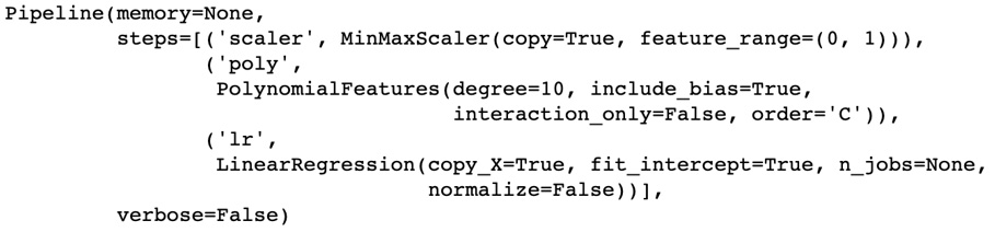
Figure 7.70: Fitting lr_model_3 on the training data
You can see from the output that the pipeline makes use of PolynomialFeatures of degree 10. You are doing this in the hope of getting a better model.
- Print out the R2 score of this model:
print('lr_model_3 R2 Score: {}'
.format(lr_model_3.score(eval_X, eval_y)))
The output of this model is similar to the following:

Figure 7.71: R2 score
You can see from the preceding figure that the R2 score is now 0.568 The previous model had an R2 score of 0.944. This model has an R2 score that is worse than the one of the previous model, lr_model_2. This happens when your model is overfitting.
- Use lr_model_3 to predict on evaluation data:
lr_model_3_preds = lr_model_3.predict(eval_X)
- Print out the MSE for lr_model_3:
print('lr_model_3 MSE: {}'
.format(mean_squared_error(eval_y, lr_model_3_preds)))
The output of this step might be similar to the following:

Figure 7.72: The MSE of lr_model_3
You can see from the preceding figure that the MSE is also worse. The MSE is 126.254, as compared to 16.271 for the previous model.
- Print out the number of coefficients (also called weights) in this model:
print(len(lr_model_3[-1].coef_))
The output might resemble the following:
1001
You can see that the model has 1,001 coefficients.
- Inspect the first 35 coefficients to get a sense of the individual magnitudes:
print(lr_model_3[-1].coef_[:35])
The output might be similar to the following:

Figure 7.73: Inspecting 35 coefficients
You can see from the output that the coefficients have significantly larger magnitudes than the coefficients from lr_model_2.
In the next steps, you will train a ridge regression model on the same set of features to reduce overfitting.
- Create a list of steps for the pipeline you will create later on:
steps = [('scaler', MinMaxScaler()),
('poly', PolynomialFeatures(degree=10)),
('lr', Ridge(alpha=0.9))]
You create a list of steps for the pipeline you will create. Note that the third step in this list is an instance of Ridge. The parameter called alpha in the call to Ridge() is the regularization parameter. You can play around with any values from 0 to 1 to see how it affects the performance of the model that you train.
- Create an instance of a pipeline:
ridge_model = Pipeline(steps)
- Fit the pipeline on the training data:
ridge_model.fit(train_X, train_y)
The output of this operation might be similar to the following:

Figure 7.74: Fitting the pipeline on training data
You can see from the output that the pipeline trained a ridge model in the final step. The regularization parameter was 0.
- Print the R2 score of ridge_model:
print('ridge_model R2 Score: {}'
.format(ridge_model.score(eval_X, eval_y)))
The output of this step might be similar to the following:

Figure 7.75: R2 score
You can see that the R2 score has climbed back up to 0.945, which is way better than the score of 0.568 that lr_model_3 had. This is already looking like a better model.
- Use ridge_model to predict on the evaluation data:
ridge_model_preds = ridge_model.predict(eval_X)
- Print the MSE of ridge_model:
print('ridge_model MSE: {}'
.format(mean_squared_error(eval_y, ridge_model_preds)))
The output might be similar to the following:

Figure 7.76: The MSE of ridge_model
You can see from the output that the MSE is 16.030, which is lower than the MSE value of 126.254 that lr_model_3 had. You can safely conclude that this is a much better model.
- Print out the number of coefficients in ridge_model:
print(len(ridge_model[-1].coef_))
The output might be similar to the following:

Figure 7.77: The number of coefficients in the ridge model
You can see that this model has 1001 coefficients, which is the same number of coefficients that lr_model_3 had.
- Print out the values of the first 35 coefficients:
print(ridge_model[-1].coef_[:35])
The output might be similar to the following:

Figure 7.78: The values of the first 35 coefficients
You can see from the preceding output that the coefficient values no longer have large magnitudes. A lot of the coefficients have a magnitude that is less than 10, with none we can see exceeding 100. This goes to show that the model is no longer overfitting.
Note
To access the source code for this specific section, please refer to https://packt.live/3248PPx.
You can also run this example online at https://packt.live/2E4LWDu.
This exercise taught you how to fix overfitting by using RidgeRegression to train a new model.
Activity 7.01: Find an Optimal Model for Predicting the Critical Temperatures of Superconductors
You work as a data scientist for a cable manufacturer. Management has decided to start shipping low-resistance cables to clients around the world. To ensure that the right cables are shipped to the right countries, they would like to predict the critical temperatures of various cables based on certain observed readings.
In this activity, you will train a linear regression model and compute the R2 score and the MSE. You will proceed to engineer new features using polynomial features of degree 3. You will compare the R2 score and MSE of this new model to those of the first model to determine overfitting. You will then use regularization to train a model that generalizes to previously unseen data.
Note
You will find the dataset required for the activity here: https://packt.live/2tJFVqu.
The original dataset can be found here: https://packt.live/3ay3aoe.
Citation:
Hamidieh, Kam, A data-driven statistical model for predicting the critical temperature of a superconductor, Computational Materials Science, Volume 154, November 2018, pages 346-354.
The steps to accomplish this task are:
- Open a Colab notebook.
- Load the necessary libraries.
- Read in the data from the superconduct folder.
- Prepare the X and y variables.
- Split the data into training and evaluation sets.
- Create a baseline linear regression model.
- Print out the R2 score and MSE of the model.
- Create a pipeline to engineer polynomial features and train a linear regression model.
- Print out the R2 score and MSE.
- Determine that this new model is overfitting.
- Create a pipeline to engineer polynomial features and train a ridge or lasso model.
- Print out the R2 score and MSE.
The output will be as follows:

Figure 7.79: The R2 score and MSE of the ridge model
- Determine that this model is no longer overfitting. This is the model to put into production.
The coefficients for the ridge model are as shown in the following figure:

Figure 7.80: The coefficients for the ridge model
Note
The solution to this activity can be found at the following address: https://packt.live/2GbJloz.
Summary
In this chapter, we studied the importance of withholding some of the available data to evaluate models. We also learned how to make use of all of the available data with a technique called cross-validation to find the best performing model from a set of models you are training. We also made use of evaluation metrics to determine when a model starts to overfit and made use of ridge and lasso regression to fix a model that is overfitting.
In the next chapter, we will go into hyperparameter tuning in depth. You will learn about various techniques for finding the best hyperparameters to train your models.