Overview
This chapter aims to show you how to track an object of your choice in an input video stream using various object trackers shipped along with the OpenCV library. We will start by understanding the basic idea behind object tracking and its applications in real life. Then, we will move on and look at the various filters present in OpenCV, understanding their algorithms, as well as their advantages and disadvantages. Finally, we will also have a look at another popular library – Dlib – and learn about the object trackers provided by it.
By the end of this chapter, you will be able to create your own tracking application where you will use cascade classifiers to track a human throughout a video using trackers such as Meanshift, CAMShift, and more. You will also carry out a comparison between trackers (Dlib-based object trackers and OpenCV object tracking API) in this chapter's activity.
Introduction
In the previous chapter, we discussed Haar Cascades and how to use them for object detection problems. We also used a variety of cascade classifiers for problems such as eye detection, people counters, and others. In this chapter, we will take this one step further and learn how to track the objects that have been detected. This tracking can be done for a pre-recorded video or a live video stream.
Object tracking is quite easy to understand. You have an object that either you have selected manually or was selected by some other algorithm, and now you want to track the object. The beauty of object tracking comes into the picture when we understand the difficulty of carrying out this very simple task in different scenarios. To understand this better, think of a scenario where you are with your friend in a busy market. Among a huge crowd, you need to detect and recognize your friend the entire time, and also need to keep track of where he or she is so that you don't end up losing them. Now, try to think of the steps that your brain is carrying out to solve this problem. First, your brain needs to coordinate with your eyes to detect humans among a large variety of objects. Then, you need to recognize your friend among many other humans, and then you need to track them continuously. There will be times when your friend will be away from you, in which case he or she will appear smaller. Similarly, sometimes, your friend will be obscured by other objects, so you must track them again once they are completely or partially visible. Now that you have understood the idea behind object tracking, you can think of scenarios where object trackers will come in handy. Whether you want to track a suspect in a video stream or track an endangered animal in a national park, such trackers can make your job easy. However, it's important to understand which tracker is suited for a specific task – how do they perform when the object you're tracking moves out of the frame and then comes back? How do they behave when the object is obscured? How much processing power do they take? How fast are they? All these questions form the base of the comparison of trackers.
In this chapter, we will start by going over the various trackers offered by the OpenCV library. We will investigate the details of each of these trackers, understanding how they work and what their advantages and disadvantages are. The chapter will consist of exercises detailing the use of trackers. We will end this chapter with an activity where we will use the cascade classifiers that we discussed in the previous chapter, along with the object trackers that we will discuss in this chapter, to create a complete object tracking application that can take input from a video stream or webcam.
Naïve Tracker
A quick disclaimer before we start this section: there is no such thing as a naïve tracker; it's just a term that we are using to describe a very basic object tracker.
Object tracking is a very popular task, so there is a huge range of deep learning-based solutions that can give very good results. Later in this chapter, we will go over those object trackers, but for now, let's start with a very basic object tracker that is based on pure and simple image processing.
The idea that we are going to target here is that if there is a clear distinction between the color of the object that you want to track and the background, then ideally, you can use basic image processing tasks such as thresholding and color spaces to track the object. Of course, this will only work when there is only one instance of the object that you want to track. This is because two similarly colored instances will both end up appearing in the tracking – which we certainly don't want.
Let's look at a frame capture from a video. We'll be performing object tracking on this image in Exercise 6.01, Object Tracking Using Basic Image Processing:

Figure 6.1: A frame capture showing a lemon falling in the water
Note
The clear distinction between the color of the lemon and the background makes it easy for us to track this object.
If you look at the preceding figure, you will notice that the lemon has a distinct yellow color compared to the black background and white bubbles. This clear difference in the color of the object and the background helps us in using simple thresholding techniques that can then be used to detect the lemon.
One more thing to note here is that while we are calling it object tracking, it's more like object detection being carried out on every frame of the video. But since there is a moving object here (in a video), we are discussing it in this chapter and not in the chapter regarding object detection.
Now, let's try to understand the concept behind this naïve tracker. The preceding image is an RGB image, which means that it has three channels – red, green, and blue. A very low value of all the three channels results in colors close to black, whereas values close to 255 for the three channels result in colors close to white. The yellow color of the lemon will lie somewhere in this range. Since we need to consider the effect of lighting, we cannot use just one RGB color value to denote the color of the lemon. So, we will start by finding out a range of pixel values that show only the lemon, and the rest of the background is converted into black. This process is nothing but thresholding. Once we have figured out that range, we can apply it to every frame of the video, separate the lemon in the video, and remove everything else. We are looking for an image that looks as follows:

Figure 6.2: The ideal result
In the preceding figure, we have separated the object (lemon) and replaced the entire background with black. Whether we can achieve this result using simple thresholding is a different question, though.
Now, let's get some hands-on experience with this technique by completing the following exercise.
Exercise 6.01: Object Tracking Using Basic Image Processing
In this exercise, we will be using a frame from a video of a lemon being dropped into water to test object tracking (considering the lemon as the object to be tracked) based on the naïve tracker algorithm/technique. We will be using the basic color space conversion that we used in Chapter 2, Common Operations When Working with Images.
Note
The video can be downloaded from https://packt.live/2YPKhck.
Perform the following steps:
- Open your Jupyter Notebook and create a new file called Exercise6.01.ipynb. We will be writing our code in this file.
- Import the OpenCV and NumPy modules:
import cv2
import numpy as np
- Create a VideoCapture object for the input video called lemon.mp4:
Note
Before proceeding, ensure that you can change the path to the video (highlighted) based on where the video is saved in your system.
# Create a VideoCapture Object
cap = cv2.VideoCapture("../data/lemon.mp4")
- Check whether the video was opened successfully or not:
if cap.isOpened() == False:
print("Error opening video")
- Create three windows. These will be used to display our input frame, our output frame, and the mask. Note that we are using the cv2.WINDOW_NORMAL flag so that we can resize the window as required. We have done this because our input video is in HD and thus the full-sized frame won't fit on our screen completely:
cv2.namedWindow("Input Video", cv2.WINDOW_NORMAL)
cv2.namedWindow("Output Video", cv2.WINDOW_NORMAL)
cv2.namedWindow("Hue", cv2.WINDOW_NORMAL)
- Create an infinite while loop for reading frames, processing them, and displaying the output frames:
while True:
- Capture a frame from the video using cap.read():
# capture frame
ret, frame = cap.read()
- Check whether the video has ended or not. This is equivalent to checking whether the frame was read successfully or not since, in a video that has finished, you can't read a new frame:
if ret == False:
break
- Now comes the main part. Convert our frame that was in the BGR color space into the HSV color space. Here, H stands for hue, S stands for saturation, and V stands for value. We are doing this so that we can easily use the hue channel for thresholding:
# Convert frame to HSV
hsv = cv2.cvtColor(frame, cv2.COLOR_BGR2HSV)
- Next, obtain the hue channel and apply thresholding. Set all the pixels that have a pixel value of more than 40 to 0 and all those that have a pixel value of less than or equal to 40 to 1:
# Obtain Hue channel
h = hsv[:,:,0]
# Apply thresholding
hCopy = h.copy()
h[hCopy>40] = 0
h[hCopy<=40] = 1
The output is as follows:

Figure 6.3: Hue channel of a frame of the video
See how the lemon is a darker color, whereas the background is comparatively lighter. That's why we are setting pixels with values more than 40 (background) to 0 and those with values less than or equal to 40 (lemon) to 1.
Note
We arrive at the value 40 by trial and error.
- Now that we have obtained the binary mask we were looking for, we will use it to keep only the lemon region in the video and replace everything else with black. Then, we will display the new mask (h), input the video frame, and output the frame subsequently:
# Display frame
cv2.imshow("Input Video", frame)
cv2.imshow("Output Video", frame*h[:,:,np.newaxis])
cv2.imshow("Hue", h*255)
- We can quit the process in the middle of it being run if we press the Esc key:
k = cv2.waitKey(10)
if k == 27:
break
- Outside of the while loop, release the VideoCapture object and close all the open display windows:
cap.release()
cv2.destroyAllWindows()
The following frames are obtained after running the program:
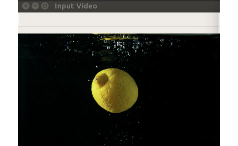
Figure 6.4: Input video frame
The following mask is obtained upon thresholding the hue channel, as performed in Step 10:

Figure 6.5: Mask obtained after thresholding the hue channel
You will obtain the following output frame after multiplying the mask by the input video frame, as performed in Step 11:

Figure 6.6: Output frame obtained after multiplying the mask by the input video frame
Note
If you look at the preceding figure, you will find that the majority of the bubbles have now been removed and that only the yellow-colored region is left.
To access the source code for this specific section, please refer to https://packt.live/2Anr88s.
If you compare Figure 6.4 and Figure 6.6 carefully, you will notice that while the bubbles have been removed in the output frame, a reflection of the lemon has remained. This is because the reflection is also yellow. This kind of issue raises a major drawback with the basic image processing-based technique we discussed earlier. While such techniques are very fast and have very low computational power requirements, they cannot be used for real-life problems since coming up with one thresholding technique and one threshold value for all videos is impossible. That's why deep learning-based techniques are heavily used for object tracking problems as they don't struggle with the aforementioned issue.
Non-Deep Learning-Based Object Trackers
In the previous section, we had a look at a very basic filter that used basic thresholding to detect objects. Tracking, in that case, was nothing but detecting an object in every frame. As we saw, this is not really object tracking, even though it might look like that, and will also fail in about every real-life scenario. In this section, we will have a look at some of the most commonly used non-deep learning-based object trackers that use motion modeling and some other techniques to track objects. We won't go into the code for these trackers here, but you can refer to the OpenCV documentation and tutorials for more information.
Kalman Filter – Predict and Update
Let's start with a tracker that also implements noise filtering and thus is referred to as a "filter." The Kalman filter was developed by Rudolf E. Kalman and Richard S. Bucy in the early 1960s. This work is more like a mechanical engineering concept rather than a core computer vision solution.
There are two main steps that are taken by the Kalman filter:
- Predict
- Update
Let's understand these steps one by one. First, let's get our terminology straight. We are going to extensively use the term system here. Now, a system, in this case, can be a ship, a person, or basically any object that you are interested in tracking. When we talk about the state of the system, we are referring to the state of motion of the system – the position and velocity of the object. Similarly, we will also talk about control inputs, which are responsible for changing the state of the system. This can be thought of as simple acceleration.
Now, recall the basic equation of the state of motion:
x= x + v * dt + 1/2 * a * dt2
Here, x is the current position of the object, dt is the time gap after which we want to find the position of the object again, v is the velocity of the object, and a is the acceleration.
If we know the velocity and acceleration of the object, we can predict the position of the object at any time step. This is the basic idea behind the predict step.
Unfortunately, in real-life scenarios, an object will change its position, velocity, and acceleration, or maybe even go out of the frame and then come back again. In such instances, it becomes impossible to predict the object's position. That's where the update step comes into the picture: whenever you encounter new information about the state of the object, you use it to initialize the predict step and then continue from there.
So, if we were to look at a basic flow diagram of this process, it would look as follows:
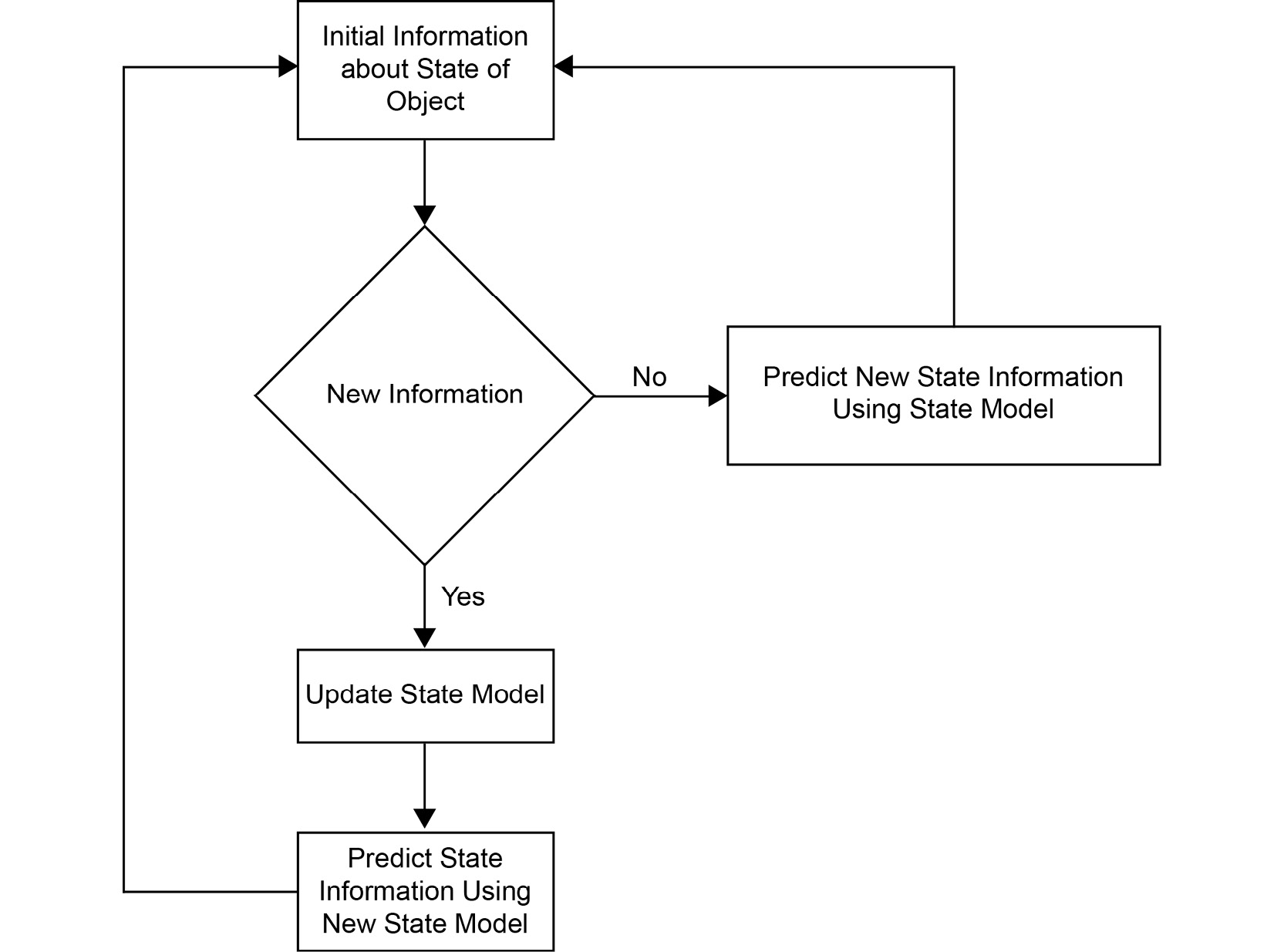
Figure 6.7: Kalman filter flowchart
Next, let's have a look at another interesting way of object tracking using a non-deep learning-based filter.
Meanshift – Density Seeking Filter
The meanshift filter is intuitive and easy to understand. It focuses on a very simple principle – we will go where the majority goes. To understand this, have a look at the following diagram. Here, the meanshift tracker keeps on following the object to be tracked (dotted circle) and can identify and track the object based on the density of the points:

Figure 6.8: Meanshift's basic process
In the following figure, you can see that the meanshift filter is seeking the "mode" (even though it has the word "mean" in its name). This means that we are tracking where most of the points lie. This is exactly how it's able to track objects.
The object it wants to track looks like a highly dense scatterplot to the filter and when that dense scatterplot moves in a frame, the meanshift filter goes after it and thus ends up tracking the object:

Figure 6.9: The way an object to be tracked looks to meanshift
The advantage of this algorithm is that since it's just looking for the mode, it does not require a specific parameter to be tuned. This is easy to understand if you think back to Haar Cascades, where we had to specify scaleFactor and minNeighbors and the results would vary based on these parameters. Here, since we are tracking a mode, there are no parameters to vary.
So far, we've discussed meanshift purely in terms of scattered points, but practically, we are going to deal with objects present in images. That's why to go from a simple image of an object to a density function (mode), we need to carry out some pre-processing. One of the ways this can be done is as follows:

Figure 6.10: Converting an object into a density function
First, we obtain a histogram of the object, which we'll use to compare our object to a new image. The result we get from this is like a density function – a higher density will mean higher chances are that the object will be present in that location. So, if we want to find where an object is present, we just have to find the spot that has the highest density function value (this is the mode).
Finally, let's have a look at the modified version of the meanshift algorithm – continuously adaptive meanshift, also known as CAMshift.
CAMshift – Continuously Adaptive Meanshift
CAMshift is a modification of meanshift that resolves the major downside of the parent algorithm – scale variation. Meanshift fails if the object's scale changes. To understand this with a real-life scenario, record yourself in a video using your mobile camera. Now, while recording, for some time, move toward the camera and then move away from the camera. In the recorded video, you will notice that as you move toward the camera, your image scale (or size) increases and that as you move away from your camera, the scale decreases. Meanshift does not give good results for this simply because it looks for the mode in a fixed-size window. This is where CAMshift comes into the picture. CAMshift uses the estimate of the mode to find out new window dimensions and then uses the new window to find the mode. This process continues until convergence is achieved, which means that the mode stops moving.
Note
One thing to note is that both meanshift and CAMshift depend a lot on convergence. They are iterative techniques and that's why, instead of finding out the object in one step, they come up with an intermediate answer that then changes further until the final location of the object is achieved. The primary difference between meanshift and CAMshift is that while meanshift keeps on going forward with these iterations while maintaining the same window size, CAMshift varies the window size, as per the intermediate result obtained, and thus can avoid any issues caused by scale variation. You can refer to the following figures to understand the difference.
Note how there is no window size variation in the following figure:

Figure 6.11: Meanshift output
Note the window size variation in the CAMshift output shown in the following figure:

Figure 6.12: CAMshift output
You might be wondering why there is no code present for meanshift, CAMshift, and the Kalman filter. The reason is that while these three techniques are quite well known and powerful, they lack the ease of use that comes with the deep learning-based models that we are going to cover next. There are implementations of these filters in OpenCV that we recommend you search for and try out yourself if you are interested in learning more.
The OpenCV Object Tracking API
OpenCV provides support for a wide range of object trackers via its object tracking API. In this section, we will start by understanding the API, the important functions that we will be using in it, and the common trackers that we can use.
Let's start with the Tracking API. If you want to read about all the functions present in the Tracking API, you can refer to the documentation here: https://docs.opencv.org/4.2.0/d9/df8/group__tracking.html.
Note
The OpenCV object tracking API is part of opencv-contrib. If you are unable to run the code given in this section, this means you have not installed OpenCV properly. You can refer to the preface for the steps on how to install OpenCV.
Just by having a brief look at the documentation page, you will see that there is a huge number of trackers available in OpenCV. Some of the common ones are as follows:
- The Boosting tracker: cv2.TrackerBoosting
- The CSRT tracker: cv2.TrackerCSRT
- GOTURN: cv2.TrackerGOTURN
- KCF (Kernelized Correlation Filter): cv2.TrackerKCF
- Median Flow: cv2.TrackerMedianFlow
- The MIL tracker: cv2.TrackerMIL
- The MOSSE (Minimum Output Sum of Squared Error) tracker: cv2.TrackerMOSSE
- The TLD (Tracking, Learning, and Detection) tracker: cv2.TrackerTLD
The interesting thing to note here is that all these trackers' functions start with cv2.Tracker. This is not really a coincidence. This is because all of these trackers have the same parent class – cv::Tracker. Because of good programming practice, all the trackers have been named in this format: cv2.Tracker<TrackerName>.
Now, before we move on and have a look at two of these trackers, let's have a look at the standard process of how to use them:
- First, depending on our use case, we will decide what tracker we will use. This is the most important step and will decide the performance of your program. Typically, the choice of a tracker is made based upon the performance speed of the tracker, including occlusion, scale variation, and so on. We will talk about this in a bit more depth when we compare the trackers shortly.
Once the tracker has been finalized, we can create the tracker object using the following function:
tracker = cv2.Tracker<TRACKER_NAME>_create()
If you are going to use the MIL tracker, for example, the preceding function will be cv2.TrackerMIL_create().
- Now, we need to tell our tracker what object we want to track. This information is provided by specifying the coordinates of the bounding box surrounding the object. Since it's difficult to specify the coordinates manually, the recommended way is to use the cv2.SelectROI function, which we used in the previous chapter to select the bounding box.
- Next, we need to initialize our tracker. While initializing, the tracker needs two things – the bounding box and the frame in which the bounding box is specified. Typically, we use the first frame for this purpose. To initialize the tracker, use tracker.init(image, bbox), where image is the frame, and bbox is the bounding box surrounding the object.
- Finally, we can start iterating over each frame of the video that we want to track our object in and update the tracker using the tracker.update(image) function, where image is the current frame that we want to find the object in. The update function returns two values – a success flag and the bounding box. If the tracker is not able to find the object, the success flag will be False. If the object is found, then the bounding box tells us where the object is present in the image.
The preceding steps have been summarized in the following flowchart:

Figure 6.13: Object tracking
Object Tracker Summary
Let's summarize the pros and cons of the object trackers we mentioned previously. You can use this information to decide which tracker to choose, depending on your use case:

Figure 6.14: Table representing the pros and cons of object trackers
As stated in the preceding table, GOTURN is a deep learning-based object tracking model and thus it requires us to download the model files. Technically speaking, the model is a Caffe model, which is why we need to download two files – the caffemodel file (model weights) and the prototxt file (model architecture). You don't need to worry about what these files are and what their purpose is. The short version of the answer is that these are the trained model weights that we will be using.
Note
You can download the prototxt file from here: https://packt.live/2YP7bRp.
Unfortunately, the caffemodel file is pretty big (~350 MB). To get that file, we will have to carry out the following steps.
We need to download the smaller zip files from the following links:
File 1: https://packt.live/2NN51ex.
File 2: https://packt.live/2Zv8aoK.
File 3: https://packt.live/2BuN2qT.
File 4: https://packt.live/3imh54s.
Next, we need to concatenate these files to form one big ZIP file:
cat goturn.caffemodel.zip* > goturn.caffemodel.zip
Windows users can use 7-zip to carry out the preceding step.
Next, unzip the ZIP file to get the goturn.caffemodel file. Both the caffemodel and prototxt files should be present in the folder where you are running your code.
Note
Unfortunately, GOTURN Tracker does not work in OpenCV 4.2.0. One option is to change to OpenCV 3.4.1 to make it work or to wait for a fix.
Now that we have seen the pros and cons of the various kinds of trackers, let's have a look at an example that shows how to use trackers in OpenCV.
Exercise 6.02: Object Tracking Using the Median Flow and MIL Trackers
Now, let's proceed with the knowledge we gained in the previous section about OpenCV's object tracking API and track an object in a video using the Median Flow and MIL trackers.
Note
Try and make some observations regarding the performance of the trackers in terms of Frames Per Second (FPS) and the way they deal with occlusions and other similar distortions.
We will be using a video of a running man to test object tracking (considering the running man as the object to be tracked) based on OpenCV's object tracking API algorithm/technique. In this exercise, we will be using the Median Flow and MIL trackers to produce the results. After evaluating the performance of these trackers, we need to decide which one works better. Follow these steps to complete this exercise:
Note
The video is available at https://packt.live/31yP2ZV.
- Create a new Jupyter Notebook and name it Exercise6.02.ipynb. We will be writing our code in this notebook.
- Import the required modules:
# Import modules
import cv2
import numpy as np
- Next, create a VideoCapture object using the cv2.VideoCapture function:
Note
Before proceeding, ensure that you can change the path to the video (highlighted) based on where the video is saved in your system.
# Create a VideoCapture Object
video = cv2.VideoCapture("../data/people.mp4")
- Check whether the video was opened successfully using the following code:
# Check if video opened successfully
if video.isOpened() == False:
print("Could not open video!")
- Next, read the first frame and also check whether we were able to read it successfully:
# Read first frame
ret, frame = video.read()
# Check if frame is read successfully
if ret == False:
print("Cannot read video")
- Display the first frame that we read:
# Show the first frame
cv2.imshow("First Frame",frame)
cv2.waitKey(0)
cv2.imwrite("firstFrame.png", frame)
The output is as follows:

Figure 6.15: First frame of the video
- Use the cv2.selectROI function to create a bounding box around the object. Print the bounding box to see the values:
# Specify the initial bounding box
bbox = cv2.selectROI(frame)
print(bbox)
The output is (41, 10, 173, 350).
- Close the window, as follows:
cv2.destroyAllWindows()
The image will look as follows:

Figure 6.16: Bounding box drawn around the person to track
- Create our tracker. Use the MedianFlow tracker, but if you want to use the MIL tracker, you just have to replace cv2.TrackerMedianFlow_create() with cv2.TrackerMIL_create():
# MedianFlow Tracker
tracker = cv2.TrackerMedianFlow_create()
- Initialize our tracker using the frame and the bounding box:
# Initialize tracker
ret = tracker.init(frame,bbox)
- Create a new display window. This is where we are going to display our tracking results:
# Create a new window where we will display
# the results
cv2.namedWindow("Tracker")
# Display the first frame
cv2.imshow("Tracker",frame)
- Next, start iterating over the frames of the video:
while True:
# Read next frame
ret, frame = video.read()
# Check if frame was read
if ret == False:
break
- Update the tracker. This will give us a flag that tells us whether the object was found or not. There will be a bounding box around the object if it was found:
# Update tracker
found, bbox = tracker.update(frame)
- If the object was found, display the bounding box around it:
# If object found, draw bbox
if found:
# Top left corner
topLeft = (int(bbox[0]), int(bbox[1]))
# Bottom right corner
bottomRight = (int(bbox[0]+bbox[2]),
int(bbox[1]+bbox[3]))
# Display bounding box
cv2.rectangle(frame, topLeft, bottomRight,
(0,0,255), 2)
- If the object was not found, display a message on the screen telling the user that the object was not found:
else:
# Display status
cv2.putText(frame, "Object not found", (20,70),
cv2.FONT_HERSHEY_SIMPLEX, 0.75, (0,0,255), 2)
- Finally, display the frame in the display window we created previously:
# Display frame
cv2.imshow("Tracker",frame)
k = cv2.waitKey(5)
if k == 27:
break
cv2.destroyAllWindows()
At this point, we recommend that you try out the different kinds of trackers that we looked at previously and see how the results change. After running the preceding code for the MIL tracker and Median Flow tracker, here's what we found.
As shown in the following figure, the trackers were able to detect the object, irrespective of the scale variation:

Figure 6.17: Object being tracked, irrespective of the scale variation
Problems arise when the object is hidden due to occlusion. While the Median Flow tracker displays that it was not able to find the object, the MIL tracker displays a false positive – a bounding box where the object is not present, as can be seen in the following figure:
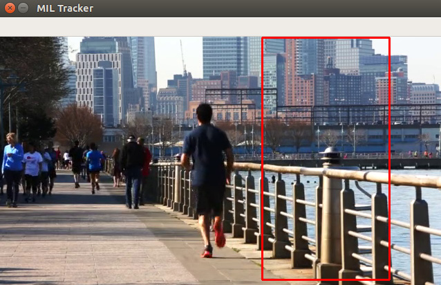
Figure 6.18: False positive given by the MIL tracker after occlusion
As shown in the following figure, the Median Flow tracker displays a message stating that it was not able to detect the object after occlusion:

Figure 6.19: Median Flow tracker displaying an "Object not found" message
In this exercise, we saw how we can use OpenCV's object tracking API to track an object that had been selected using OpenCV's selectROI function. We also saw how easy it is to use the API: all we need to do is replace one tracker with another and the rest of the code will stay the same.
Note
To access the source code for this specific section, please refer to https://packt.live/2YPSa1D.
So far, we have been talking about OpenCV's object tracking API. Now, let's have a look at another popular computer vision library – dlib. First, we will install Dlib and then use it to carry out object tracking in the upcoming sections.
Installing Dlib
Since we will be discussing object tracking using Dlib, let's see how we can install it. We will use the recommended approach of installing Dlib using the following pip command:
pip install dlib
You should be able to see the following on your Command Prompt or Terminal, depending on your operating system:

Figure 6.20: Output of the pip install dlib command
Once the installation is successful, you will see the following message on your screen:
Figure 6.21: Output after Dlib installation is complete
Note
Note that dlib is a very heavy module and can take a lot of time and RAM during installation. So, if your system appears to be stuck during the installation process, there is no need to panic. Typically, installation can take anywhere between 5 to 20 minutes.
We can check whether the installation was successful or not by trying to import dlib, as follows:
- Open your Command Prompt or Terminal and type python.
- In the Python shell, enter import dlib to import the dlib module.
- Finally, print the version of Dlib that has been installed using print(dlib.__version__).
The output of the preceding commands is shown in the following screenshot:

Figure 6.22: Verifying the Dlib installation by printing the version of dlib that's installed
If you can see the preceding output, then you have successfully installed Dlib. Now, let's learn how to use Dlib for object tracking.
Object Tracking Using Dlib
Dlib's object tracking algorithm is built upon the MOSSE tracker. If you refer to the object tracker summary we provided previously, you will notice that MOSSE doesn't have the best performance when there is scale variation. To cater for this, Dlib's object tracking algorithm uses the technique described in the paper Accurate Scale Estimation for Robust Visual Tracking, which was published in 2014.
Note
Citation: Martin Danelljan, Gustav Häger, Fahad Shahbaz Khan, and Michael Felsberg. Accurate Scale Estimation for Robust Visual Tracking. Proceedings of the British Machine Vision Conference 2014, 2014. https://doi.org/10.5244/c.28.65.
This technique involves estimating the scale of the object after every update step. Because of this, we can now deal with scale variation and utilize the pros of the MOSSE tracker. The following flowchart demonstrates the object tracking process when using Dlib:

Figure 6.23: Object tracking using Dlib
Let's have a look at the process of using object tracking in Dlib. Notice how the first few steps remain the same as when using object tracking in OpenCV.
First, we'll need to import the dlib module into our code:
import dlib
Next, just like in OpenCV, we will have to create a bounding box around the object that we want to track, but only for the first time that we do this. For this, we can use the cv2.selectROI function.
Now comes a very important point. Dlib uses images in RGB format, whereas OpenCV uses images in BGR format. So, we need to convert images that have been loaded by OpenCV into RGB format using the following code:
rgb = cv2.cvtColor(bgr, cv2.COLOR_BGR2RGB)
Next, we will also need to convert the rectangle given by the cv2.selectROI function into Dlib's rectangle type, as follows:
topLeftX, topLeftY, w, h) = bbox
bottomRightX = topLeftX+w
bottomRightY = topLeftY+h
dlibRect = dlib.rectangle(topLeftX, topLeftY,
bottomRightX, bottomRightY)
Now, we can create our dlib tracker, as follows:
tracker = dlib.correlation_tracker()
Since we have the tracker ready, we can start the tracking process. The first time we do this, we will have to provide the bounding box around the object and the image:
tracker.start_track(rgb, dlibRect)
For the later frames, we can directly update the tracker and get the position of the object. Again, we'll need to make sure that we are using RGB frames here:
tracker.update(rgb)
objectPosition = tracker.get_position()
objectPosition is an instance of the Dlib rectangle. So, we need to convert it back into OpenCV's rectangle format so that we can create a bounding box using the cv2.rectangle command:
topLeftX = int(objectPosition.left())
topLeftY = int(objectPosition.top())
bottomRightX = int(objectPosition.right())
bottomRightY = int(objectPosition.bottom())
Finally, to draw the rectangle, we can use the cv2.rectangle command, as we did in the previous chapter:
cv2.rectangle(rgb, (topLeftX, topLeftY), (bottomRightX, bottomRightY),
(0,0,255), 2)
And that's it. That's all you need to do to carry out object tracking using Dlib. Now, let's strengthen our understanding of this process with the help of an example. You can also refer to Figure 6.23 as a quick reference to the preceding process.
Exercise 6.03: Object Tracking Using Dlib
As a continuation of Exercise 6.02, Object Tracking Using the Median Flow and MIL Trackers, we will track the running man based on the Dlib technique/algorithm and use a modified MOSSE tracker to analyze the performance with respect to the same parameters that we calculated earlier. Also, we will evaluate the performance in comparison with the trackers used in Exercise 6.02, Object Tracking Using the Median Flow and MIL Trackers. As we saw previously, the video has lighting changes, partial and complete occlusion, and scale variation. This will help you compare the three trackers using a total of four aspects – performance in terms of FPS and their ability to deal with the three issues – lighting change, occlusion, and scale variation. We will leave this as an open exercise for you to try out yourself. See whether your observations match the observations we stated previously in this chapter. Follow these steps to complete this exercise:
Note
The video is available at https://packt.live/31yP2ZV.
Perform the following steps:
- Import the required modules (OpenCV, NumPy, and Dlib):
# Import modules
import cv2
import numpy as np
import dlib
- Create a VideoCapture object and see whether the video was loaded successfully:
Note
Before proceeding, ensure that you can change the path to the video (highlighted) based on where the video is saved in your system.
# Create a VideoCapture Object
video = cv2.VideoCapture("../data/people.mp4")
# Check if video opened successfully
if video.isOpened() == False:
print("Could not open video!")
- Next, read the first frame and check whether it was read successfully:
# Read first frame
ret, frame = video.read()
# Check if frame read successfully
if ret == False:
print("Cannot read video")
- Now, display the first frame and then select the ROI:
# Show the first frame
cv2.imshow("First Frame",frame)
cv2.waitKey(0)
# Specify the initial bounding box
bbox = cv2.selectROI(frame)
cv2.destroyAllWindows()
- Convert the frame into RGB since that's what Dlib uses:
# Convert frame to RGB
rgb = cv2.cvtColor(frame,cv2.COLOR_BGR2RGB)
- Convert the rectangle into a Dlib rectangle:
# Convert bbox to Dlib rectangle
(topLeftX, topLeftY, w, h) = bbox
bottomRightX = topLeftX + w
bottomRightY = topLeftY + h
dlibRect = dlib.rectangle(topLeftX, topLeftY,
bottomRightX, bottomRightY)
- Create the tracker and initialize it using the Dlib rectangle and the RGB frame:
# Create tracker
tracker = dlib.correlation_tracker()
# Initialize tracker
tracker.start_track(rgb, dlibRect)
- Create a new display window. This is where we will be displaying our tracking output:
# Create a new window where we will display the results
cv2.namedWindow("Tracker")
# Display the first frame
cv2.imshow("Tracker",frame)
- Start iterating over the frames of the video:
while True:
# Read next frame
ret, frame = video.read()
# Check if frame was read
if ret == False:
break
- Convert the frame that we just read into RGB:
# Convert frame to RGB
rgb = cv2.cvtColor(frame,cv2.COLOR_BGR2RGB)
- Update the tracker so that it can find the object:
# Update tracker
tracker.update(rgb)
- Use the position given by the tracker to create a bounding box over the detected object:
objectPosition = tracker.get_position()
topLeftX = int(objectPosition.left())
topLeftY = int(objectPosition.top())
bottomRightX = int(objectPosition.right())
bottomRightY = int(objectPosition.bottom())
# Create bounding box
cv2.rectangle(frame, (topLeftX, topLeftY), (bottomRightX,
bottomRightY), (0,0,255), 2)
- Finally, display the frame on the display window we created previously:
# Display frame
cv2.imshow("Tracker",frame)
k = cv2.waitKey(5)
if k == 27:
break
cv2.destroyAllWindows()
The output is as follows:

Figure 6.24: Dlib object tracking output
Notice how the Dlib object tracking algorithm was able to accurately track the object of interest, unlike the two algorithms we discussed in the previous exercise. This does not mean that this algorithm is superior compared to the other two. It only means that it's a more suitable choice for the specific case study we are talking about. Such experiments are hugely important in the computer vision domain.
Note
To access the source code for this specific section, please refer to https://packt.live/2ZvbVKS.
So, in this exercise, we saw how we can use an object tracker using Dlib. Now, to wrap up this chapter, let's consider a practical case study. This will be especially fun for people who either love playing football or watching it.
Activity 6.01: Implementing Autofocus Using Object Tracking
In the previous chapter, we discussed face detection using Haar Cascades and also mentioned that we could use frontal face cascades to implement the autofocus feature in cameras. In this activity, we will implement an autofocus utility (we discussed it briefly in Chapter 5, Face Processing in Image and Video) that can be used in football to track the ball throughout the game. Now, while this might appear very strange at first, such a feature could come in handy. Right now, cameramen have to pan their cameras wherever the ball is and that becomes a cumbersome job. If we had an autofocus utility that could track the ball throughout the game, the camera could pan automatically to follow the ball. We will be using a video of a local football game. We want you to try out the two computer vision libraries we have covered so far – OpenCV and Dlib – for object tracking and see which specific algorithm gives you the best result in this case. This way, you will get a chance to carry out the experimentation that we discussed previously, after Exercise 6.02, Object Tracking Using the Median Flow and MIL Trackers. We've also included an additional challenge for you to try out on your own. Follow these steps to complete this activity:
- Open your Jupyter Notebook and create a new file called Activity6.01.ipynb. We will be writing our code in this notebook. Also, use the Exercise6.02.ipynb and Exercise6.03.ipynb files as references for this activity.
- First, import the necessary libraries – OpenCV, NumPy, and Dlib.
- Next, create a VideoCapture object by reading the video file present at ../data/soccer2.mp4.
Note
The video can be downloaded from https://packt.live/2NHXwpp.
- Check whether the video was loaded successfully.
- Next, we will read the first frame and verify whether we were able to read the frame properly or not.
- Now that we have read the frame, we can display it to see whether everything has worked fine so far.
- Next, select the ROI (the bounding box around the football) using the cv2.selectROI function. In this case, we will be using OpenCV's object trackers for object tracking, but it is recommended to try both OpenCV and Dlib's object trackers.
- Create an object tracker using the functions we used previously. Use proper experimentation to find out which object tracker gives the best performance.
- Once the object tracker has been created, we can initialize it using the bounding box we created in Step 7 and the first frame.
- Next, create a display window to display the tracking output.
- Now, you can use the same while loop that we used in Exercise6.02.ipynb to iterate over each frame, thus updating the tracker and displaying a bounding box around the object.
- Once you are out of the while loop, close all the display windows.
The following figure shows the output that will be obtained for OpenCV's selectROI function, which is used to select the object (football) that we want to track:

Figure 6.25: ROI selection
The output of the object tracker will be as follows for one of the frames of the video. This will appear inside the while loop, which is where you will display the object's position that was obtained using the object tracker:
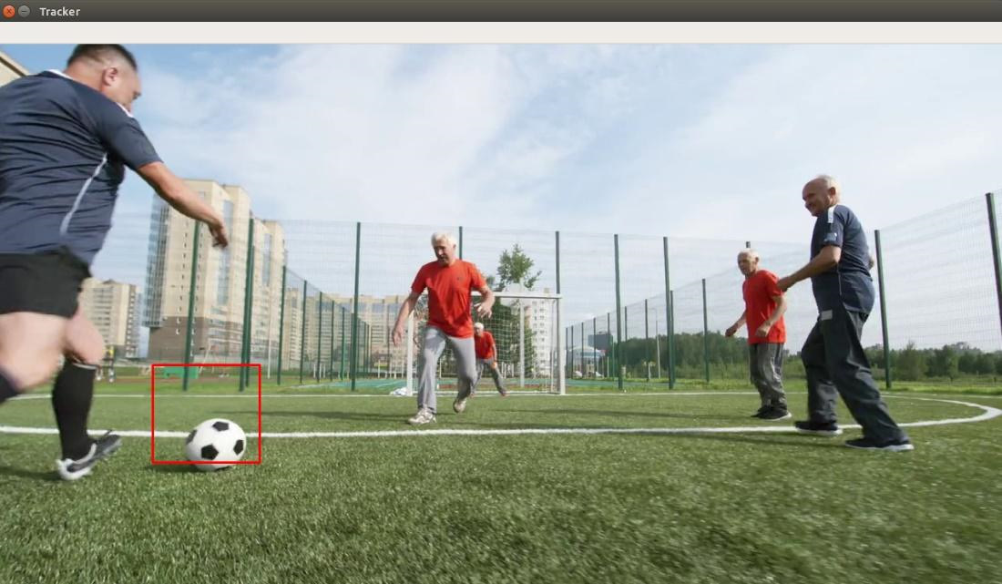
Figure 6.26: Output of the object tracker
Additional Challenge:
At this point, we want you to think about why such a simple object tracking program will fail in real life. We have got two kinds of trackers – ones that are very strict, which means that even if they have a slight doubt about the object, they will just say that the object was not found, and then we have got trackers such as the Dlib object tracker and the TLD object tracker, which give a lot of false positives. This calls for a hybrid tracker pipeline. The basic idea behind this is that we will use the strict object tracker to track the object and if the object is not detected, we will switch to the other object tracker to provide the location of the object. The advantage of such an approach is that for most frames, you will get a very accurate location of the object and when the strict object tracker fails, the other object tracker will still be able to give some information about the object's location. We recommend that you think about this approach more deeply and implement it on your own.
Note
The solution for this activity can be found on page 513.
In this activity, we saw how we can use different trackers based on the situation we are dealing with. The best part of using the OpenCV object tracking API is that it requires minimal code changes when shifting from one tracker to another. It is recommended that you try using other trackers supported by OpenCV on this case study and carry out a comparison between them.
Summary
This was our first advanced computer vision topic where we used statistical and deep learning-based object tracking models to solve case studies involving object surveillance and other similar examples. We started with a very basic object tracker that was based on a very naive approach. We also saw how the tracker, while computationally very cheap, has very low performance and can't be used for most real-life scenarios. We used the HSV color space in Exercise 6.01, Object Tracking Using Basic Image Processing, to track a lemon across various frames on the input video. We then went ahead and discussed common non-deep learning-based trackers – the Kalman filter and the meanshift and CAMshift filters. Next, we discussed the OpenCV object tracking API, where we listed the eight commonly used object trackers and their pros and cons. We also had a look at how we can use those trackers and how GOTURN requires a slightly different process since we need to download the Caffe model and the prototxt file. We learned how to use these object trackers in Exercise 6.02, Object Tracking Using the Median Flow and MIL Trackers, where we tracked a jogger across various frames in a video. We also saw how we can shift between different object trackers with the help of OpenCV's object tracking API. We then went ahead and discussed Dlib, which is another well-known and commonly used computer vision library by Davis King. We saw how we can use object tracking using Dlib. Finally, we wrapped up this chapter by having a look at an activity involving tracking the ball in a football game. In the next chapter, we will talk about object detection and face recognition. The importance of this topic can be understood by the fact that, right now, we have to manually provide the bounding box, but with the help of an object detection pipeline, we can automate the process of finding an object in a frame and then track it in the subsequent frames.