Overview
This chapter serves as an introduction to the amazing and colorful world of image processing. We will start by understanding images and their various components – pixels, pixel values, and channels. We will then have a look at the commonly used color spaces – red, green, and blue (RGB) and Hue, Saturation, and Value (HSV). Next, we will look at how images are loaded and represented in OpenCV and how can they be displayed using another library called Matplotlib. Finally, we will have a look at how we can access and manipulate pixels. By the end of this chapter, you will be able to implement the concepts of color space conversion.
Introduction
Welcome to the world of images. It's interesting, it's wide, and most importantly, it's colorful. The world of artificial intelligence (AI) is impacting how we, as humans, can use the power of smart computers to perform tasks much faster, more efficiently, and with minimal effort. The idea of imparting human-like intelligence to computers (known as AI) is a really interesting concept. When the intelligence is focused on images and videos, the domain is referred to as computer vision. Similarly, natural language processing (NLP) is the AI stream where we try to understand the meaning behind the text. This technology is used by major companies for building AI-based chatbots designed to interact with customers. Both computer vision and NLP share the concepts of deep learning, where we use deep neural networks to complete tasks such as object detection, image classification, word embedding, and more. Coming back to the topic of computer vision, companies have come up with interesting use cases where AI systems have managed to change entire scenarios. Google, for example, came up with the idea of Google Goggles, which can perform several operations, such as image classification, object recognition, and more. Similarly, Tesla's self-driving cars use computer vision extensively to detect pedestrians and vehicles on the road and to detect the lane on which the car is moving.
This book will serve as a journey through the interesting components of computer vision. We will start by understanding images and then go over how they can be processed. After a couple of chapters, we will jump into detailed topics such as histograms and contours and finally go over some real-life applications of computer vision – face processing, object detection, object tracking, 3D reconstruction, and so on. This is going to be a long journey, but we will get through it together.
We love looking at high-resolution color photographs, thanks to the gamut of colors they offer. Not so long ago, however, we had photos printed only in black and white. However, those "black-and-white" photos also had some color in them, the only difference being that the colors were all shades of gray. The common thing that's there in all these components is the vision part. That's where computer vision gets its name. Computer refers to the fact that it's the computer that is processing the visual data, while vision refers to the fact that we are dealing with visual data – images and videos.
An image is made up of smaller components called pixels. A video is made up of multiple frames, each of which is nothing but an image. The following diagram gives us an idea of the various components of videos, images, and pixels:
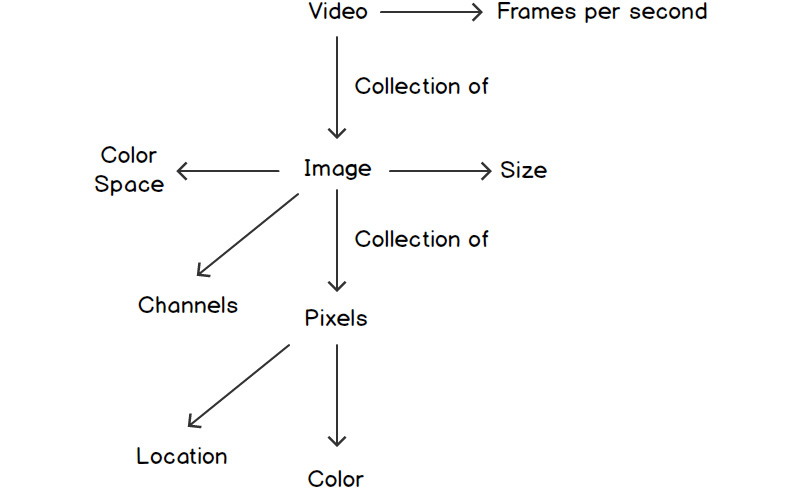
Figure 1.1: Relationships between videos, images, and pixels
In this chapter, we will focus only on images and pixels. We will also go through an introduction to the OpenCV library, along with the functions present in the library that are commonly used for basic image processing. Before we jump into the details of images and pixels, let's get through the prerequisites, starting with NumPy arrays. The reason behind this is that images in OpenCV are nothing but NumPy arrays. Just as a quick recap, NumPy is a Python module that's used for numerical computations and is well known for its high-speed computations.
NumPy Arrays
Let's learn how to create a NumPy array in Python.
First, we need to import the NumPy module using the import numpy as np command. Here, np is used as an alias. This means that instead of writing numpy.function_name, we can use np.function_name.
We will have a look at four ways of creating a NumPy array:
- Array filled with zeros – the np.zeros command
- Array filled with ones – the np.ones command
- Array filled with random numbers – the np.random.rand command
- Array filled with values specified – the np.array command
Let's start with the np.zeros and np.ones commands. There are two important arguments for these functions:
- The shape of the array. For a 2D array, this is (number of rows, number of columns).
- The data type of the elements. By default, NumPy uses floating-point numbers for its data types. For images, we will use unsigned 8-bit integers – np.uint8. The reason behind this is that 8-bit unsigned integers have a range of 0 to 255, which is the same range that's followed for pixel values.
Let's have a look at a simple example of creating an array full of zeros. The array size should be 4x3. We can do this by using np.zeros(4,3). Similarly, if we want to create a 4x3 array full of ones, we can use np.ones(4,3).
The np.random.rand function, on the other hand, only needs the shape of the array. For a 2D array, it will be provided as np.random.rand(number_of_rows, number_of_columns).
Finally, for the np.array function, we provide the data as the first argument and the data type as the second argument.
Once you have a NumPy array, you can use npArray.shape to find out the shape of the array, where npArray is the name of the NumPy array. We can also use npArray.dtype to display the data type of the elements in the array.
Let's learn how to use these functions by completing the first exercise of this chapter.
Exercise 1.01: Creating NumPy Arrays
In this exercise, we will get some hands-on experience with the various NumPy functions that are used to create NumPy arrays and to obtain their shape. We will be using NumPy's zeros, ones, and rand functions to create the arrays. We will also have a look at their data types and shapes. Follow these steps to complete this exercise:
- Create a new notebook and name it Exercise1.01.ipynb. This is where we will write our code.
- First, import the NumPy module:
import numpy as np
- Next, let's create a 2D NumPy array with 5 rows and 6 columns, filled with zeros:
npArray = np.zeros((5,6))
- Let's print the array we just created:
print(npArray)
The output is as follows:
[[0. 0. 0. 0. 0. 0.]
[0. 0. 0. 0. 0. 0.]
[0. 0. 0. 0. 0. 0.]
[0. 0. 0. 0. 0. 0.]
[0. 0. 0. 0. 0. 0.]]
- Next, let's print the data type of the elements of the array:
print(npArray.dtype)
The output is float64.
- Finally, let's print the shape of the array:
print(npArray.shape)
The output is (5, 6).
- Print the number of rows and columns in the array:
Note
The code snippet shown here uses a backslash ( ) to split the logic across multiple lines. When the code is executed, Python will ignore the backslash, and treat the code on the next line as a direct continuation of the current line.
print("Number of rows in array = {}"
.format(npArray.shape[0]))
print("Number of columns in array = {}"
.format(npArray.shape[1]))
The output is as follows:
Number of rows in array = 5
Number of columns in array = 6
- Notice that the array we just created used floating-point numbers as the data type. Let's create a new array with another data type – an unsigned 8-bit integer – and find out its data type and shape:
npArray = np.zeros((5,6), dtype=np.uint8)
- Use the print() function to display the contents of the array:
print(npArray)
The output is as follows:
[[0 0 0 0 0 0]
[0 0 0 0 0 0]
[0 0 0 0 0 0]
[0 0 0 0 0 0]
[0 0 0 0 0 0]]
- Print the data type of npArray, as follows:
print(npArray.dtype)
The output is uint8.
- Print the shape of the array, as follows:
print(npArray.shape)
The output is (5, 6).
Note
The code snippet shown here uses a backslash ( ) to split the logic across multiple lines. When the code is executed, Python will ignore the backslash, and treat the code on the next line as a direct continuation of the current line.
- Print the number of rows and columns in the array, as follows:
print("Number of rows in array = {}"
.format(npArray.shape[0]))
print("Number of columns in array = {}"
.format(npArray.shape[1]))
The output is as follows:
Number of rows in array = 5
Number of columns in array = 6
- Now, we will create arrays of the same size, that is, (5,6), and the same data type (an unsigned 8-bit integer) using the other commands we saw previously. Let's create an array filled with ones:
npArray = np.ones((5,6), dtype=np.uint8)
- Let's print the array we have created:
print(npArray)
The output is as follows:
[[1 1 1 1 1 1]
[1 1 1 1 1 1]
[1 1 1 1 1 1]
[1 1 1 1 1 1]
[1 1 1 1 1 1]]
- Let's print the data type of the array and its shape. We can verify that the data type of the array is actually a uint8:
print(npArray.dtype)
print(npArray.shape)
The output is as follows:
uint8
(5, 6)
- Next, let's print the number of rows and columns in the array:
print("Number of rows in array = {}"
.format(npArray.shape[0]))
print("Number of columns in array = {}"
.format(npArray.shape[1]))
The output is as follows:
Number of rows in array = 5
Number of columns in array = 6
- Next, we will create an array filled with random numbers. Note that we cannot specify the data type while building an array filled with random numbers:
npArray = np.random.rand(5,6)
- As we did previously, let's print the array to find out the elements of the array:
print(npArray)
The output is as follows:
[[0.19959385 0.36014215 0.8687727 0.03460717 0.66908867 0.65924373] [0.18098379 0.75098049 0.85627628 0.09379154 0.86269739 0.91590054] [0.79175856 0.24177746 0.95465331 0.34505896 0.49370488 0.06673543] [0.54195549 0.59927631 0.30597663 0.1569594 0.09029267 0.24362439] [0.01368384 0.84902871 0.02571856 0.97014665 0.38342116 0.70014051]]
- Next, let's print the data type and shape of the random array:
print(npArray.dtype)
print(npArray.shape)
The output is as follows:
float64
(5, 6)
- Finally, let's print the number of rows and columns in the array:
print("Number of rows in array = {}"
.format(npArray.shape[0]))
print("Number of columns in array = {}"
.format(npArray.shape[1]))
The output is as follows:
Number of rows in array = 5
Number of columns in array = 6
- Finally, let's create an array that looks like the one shown in the following figure:

Figure 1.2: NumPy array
The code to create and print the array is as follows:
npArray = np.array([[1,2,3,4,5,6],
[7,8,9,10,11,12],
[13,14,15,16,17,18],
[19,20,21,22,23,24],
[25,26,27,28,29,30]],
dtype=np.uint8)
print(npArray)
The output is as follows:
[[ 1 2 3 4 5 6]
[ 7 8 9 10 11 12]
[13 14 15 16 17 18]
[19 20 21 22 23 24]
[25 26 27 28 29 30]]
- Now, just like in the previous cases, we will print the data type and the shape of the array:
print(npArray.dtype)
print(npArray.shape)
print("Number of rows in array = {}"
.format(npArray.shape[0]))
print("Number of columns in array = {}"
.format(npArray.shape[1]))
The output is as follows:
uint8
(5, 6)
Number of rows in array = 5
Number of columns in array = 6
In this exercise, we saw how to create NumPy arrays using different functions, how to specify their data types, and how to display their shape.
Note
To access the source code for this specific section, please refer to https://packt.live/3ic9R30.
Now that we are armed with the prerequisites, let's formally jump into the world of image processing by discussing the building blocks of images – pixels.
Pixels in Images
By now, we know that images are made up of pixels. Pixels can be thought of as very small, square-like structures that, when joined, result in an image. They serve as the smallest building blocks of any image. Let's take an example of an image. The following image is made up of millions of pixels that are different colors:

Figure 1.3: An image of a lion and a girl
Note
Image source: https://www.pxfuel.com/en/free-photo-olgbr.
Let's see what pixels look like up close. What happens when we keep on zooming in on the girl's eye in the image? After a certain point, we will end up with something like the following:
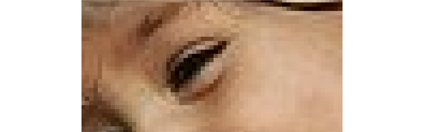
Figure 1.4: Highly zoomed-in version of the image shown in Figure 1.3
If you look carefully at the preceding image, you will be able to see some squares in the image. These are known as pixels. A pixel does not have a standard size; it differs from device to device. We frequently use the term pixels per inches (PPI) to define the resolution of an image. More pixels in an inch (or square inch) of an image means a higher resolution. So, an image from a DSLR has more pixels per inch, while an image from a laptop webcam will have fewer pixels per inch. Let's compare the image we saw in Figure 1.4 with its higher-resolution version (Figure 1.5). We'll notice how, in a higher-resolution image, we can zoom in on the same region and have a much better quality image compared to the lower-resolution image (Figure 1.4):

Figure 1.5: Same zoomed-in region for a higher-resolution image
Now that we have a basic idea of pixels and terms such as PPI and resolution, let's understand the properties of pixels – pixel location and the color of the pixel.
Pixel Location – Image Coordinate System
We know that a pixel is a square and is the smallest building block of an image. A specific pixel is referenced using its location in the image. Each image has a specific coordinate system. The standard followed in OpenCV is that the top-left corner of an image acts as the origin, (0,0). As we move to the right, the x-coordinate of the pixel location increases, and as we move down, the y-coordinate increases. But it's very important to understand that this is not a universally followed coordinate system. Let's try to follow a different coordinate system for the time being. We can find out the location of a pixel using this coordinate system.
Let's consider the same image (Figure 1.3) that we looked at previously and try to understand its coordinate system:
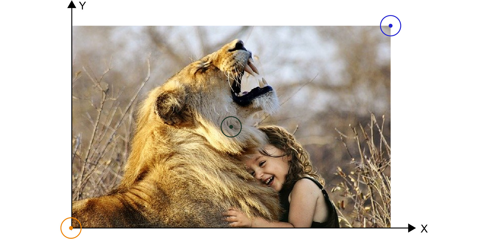
Figure 1.6: Image coordinate system
We have the same image as before and we have added the two axes – an X axis and a Y axis. The X axis is the horizontal axis, while the y-axis is the vertical axis. The origin of this coordinate system lies at the bottom-left corner of the image. Armed with this information, let's find the coordinates of the three points marked in the preceding figure – the orange point (at the bottom left), the green point (at the center of the image), and the blue point (at the top right of the image).
We know that the orange point lies at the bottom-left corner of the image, which is exactly where the origin of the image's coordinate system lies. So, the coordinates of the pixel at the bottom-left corner are (0,0).
What about the blue point? Let's assume that the width of the image is W and the height of the image is H. By doing this, we can see that the x coordinate of the blue point will be the width of the image, (W), while the y coordinate will be the height of the image, (H). So, the coordinates of the pixel at the top-right corner are (W, H).
Now, let's think about the coordinates for the center point. The x coordinate of the center will be W/2, while the y coordinate of the point will be H/2. So, the coordinates of the pixel at the center are (W/2, H/2).
Can you find the coordinates of any other pixels in the image? Try this as an additional challenge.
So, now we know how to find a pixel's location. We can use this information to extract information about a specific pixel or a group of pixels.
There is one more property associated with a pixel, and that is its color. But, before we take a look at that, let's look at the properties of an image.
Image Properties
By now, we have a very good idea of images and pixels. Now, let's understand the properties of an image. From Figure 1.1, we can see that there are three main properties (or attributes) of an image – image size, color space, and the number of channels in an image. Let's explore each property in detail.
Size of the Image
First, let's understand the size of the image. The size of an image is represented by its height and width. Let's understand this in detail.
There are quite a few ways of referring to the width and height of an image. If you have filled in any government forms, you will know that a lot of the time, they ask for images with dimensions such as 3.5 cm×4.5 cm. This means that the width of the image will be 3.5 cm and the height of the image will be 4.5 cm.
However, when you try downloading images from websites such as Pixabay (https://pixabay.com/), you get options such as the following ones:
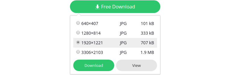
Figure 1.7: Image dimensions on Pixabay
So, what happened here? Are these numbers in centimeters or millimeters, or some other unit? Interestingly, these numbers are in pixels. These numbers represent the number of pixels that are present in the image. So, an image with size 1920×1221 will have a total of 1920×1221 = 2334420 pixels. These numbers are sometimes related to the resolution of the image as well. A higher number of pixels in an image means that the image has more detail, or in other words, we can zoom into the image more without losing its detail.
Can you try to figure out when you would need to use which image size representation? Let's try to get to the bottom of this by understanding the use cases of these different representations.
When you have your passport-size photo printed out so that you can paste it in a box in a form, you are more concerned about the size of the image in terms of units such as centimeters. Why? Because you want the image to fit in the box. Since we are talking about the physical world, the dimensions are also represented in physical units such as centimeters, inches, or millimeters. Will it matter to you how many pixels the image is made up of at that time? Consider the following form, which is where we are going to paste a passport-size photo:

Figure 1.8: A sample form where an image must be pasted
But what about an image that's in soft copy form? Let's take the following two images as an example:
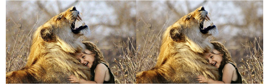
Figure 1.9: Two images with the same physical dimensions
Both of the preceding images have the same physical dimensions – a height of 2.3 inches and a width of 3.6 inches. So, are they the same images? The answer is no. The image on the left has a much higher number of pixels compared to the image on the right. This difference is evident when you are more focused on the details (or resolution) of the image rather than the physical dimensions of the image.
For example, the profile photo of every user on Facebook has the same dimensions when viewed alongside a post or a comment. But that does not mean that every image has the same sharpness/resolution/detail. Notice how we have used three words here – sharpness, resolution, and detail – to convey the same sense, that is, the quality of the image. An image with a higher number of pixels will be of far better quality compared to the same image with a lower number of pixels. Now, what kind of dimensions will we use in our book? Since we are dealing with soft copies of images, we will represent the size of images using the number of pixels in them.
Now, let's look at what we mean by color spaces and channels of an image.
Color Spaces and Channels
Whenever we look at a color image as humans, we are looking at three types of color, or attributes. But what three colors or attributes? Consider the two images given below. Both of them look very different but the interesting thing is that they are actually just two different versions of the same image. The difference is the color space they are represented in. Let's understand this with an analogy. We have a wooden chair. Now the wood used can be different, but the chair will still be the same. It's the same thing here. The image is the same, just the color space is different.
Let's understand this in detail. Here, we have two images:

Figure 1.10: Same images with different color spaces
While the image on the left uses red, green, and blue as the three attributes, thereby making its color space the RGB color space, the image on the left uses hue, saturation, and value as the three attributes, thereby making its color space the HSV color space.
At this point, you might be thinking, "why do we need different color spaces?" Well, since different color spaces use different attributes, depending on the problem we want to solve, we can use a color space that focuses on a certain attribute. Let's take a look at an example:

Figure 1.11: The red, green, and blue channels of an image
In the preceding figure, we have separated the three attributes that made the color space of the image – red, green, and blue. These attributes are also referred to as channels. So, the RGB color space has three channels – a red channel, a green channel, and a blue channel. We will understand why these images are in grayscale soon.
Similarly, let's consider the three channels of the HSV color space – hue, saturation, and value:
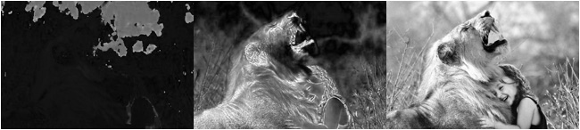
Figure 1.12: The hue, saturation, and value channels of an HSV image
Now, compare the results shown in Figure 1.11 and Figure 1.12. Let's propose a problem. Let's say that we want to detect the edges present in an image. Why? Well, edges are responsible for details in an image. But we won't go into the details of that right now. Let's just assume that, for some reason, we want to detect the edges in an image. Purely based on visualization, you can see that the saturation channel of the HSV image already has a lot of edges highlighted, so even if we don't do any processing and go ahead and use the saturation channel of the HSV image, we will end up with a pretty good start for the edges.
This is exactly why we need color spaces. When we just want to see an image and praise the photographer, the RGB color space is much better than the HSV color space. But when we want to detect edges, the HSV color space is better than the RGB color space. Again, this is not a general rule and depends on the image that we are talking about.
Sometimes, the HSV color space is preferred over the RGB color space. The reason behind this is that the red, green, and blue components (or channels) in the RGB color space have a high correlation between them. The HSV color space, on the other hand, allows us to separate the value channel of the image entirely, which helps us in processing the image. Consider a case of object detection where you want to detect an object present in an image. In this problem, you will want to make sure that light invariance is present, meaning that the object can be detected irrespective of whether the image is dark or bright. Since the HSV color space allows us to separate the value or intensity channel, it's better to use it for this object detection case study.
It's also important to note that we have a large variety of color spaces; RGB and HSV are just two of them. At this point, it's not important for you to know all the color spaces. But if you are interested, you can refer to the color spaces supported by OpenCV and how an image from one color space is converted into another color space here: https://docs.opencv.org/4.2.0/de/d25/imgproc_color_conversions.html.
Let's have a look at another color space – grayscale. This will also answer your question as to why the red, green, and blue channels in Figure 1.11 don't look red, green, and blue, respectively.
When an image has just one channel, we say that it's in grayscale mode. This is because the pixels are color in shades of gray depending on the pixel value. A pixel value of 0 represents black, whereas a pixel value of 255 represents white. You'll learn more about this in the next section.
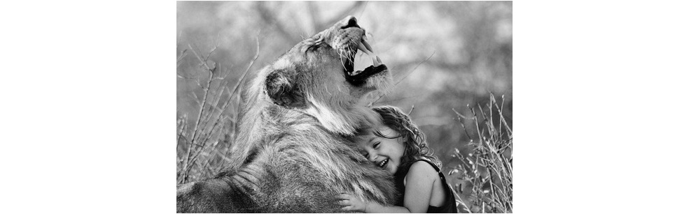
Figure 1.13: Image in grayscale mode
When we divided the RGB and HSV images into their three channels, we were left with images that had only one channel each, and that's why they were converted into grayscale and were colored in this shade of gray.
In this section, we learned what we mean by the color space of an image and what a channel means. Now, let's look at pixel values in detail.
Pixel Values
So far, we have discussed what pixels are and their properties. We learned how to represent a pixel's location using image coordinate systems. Now, we will learn how to represent a pixel's value. First, what do we mean by a pixel's value? Well, a pixel's value is nothing but the color present in that pixel. It's important to note here that a pixel can have only one color. That's why a pixel's value is a fixed value.
If we talk about an image in grayscale, a pixel value can range between 0 and 255 (both inclusive), where 0 represents black and 255 represents white.
Note
In the following figure, there are two axes: X and Y. These axes represent the width and height of the image, respectively, and don't hold much importance in the computer vision domain. That's why they can be safely ignored. Instead, it's important to focus on the pixel values in the images.
Refer to Figure 1.14 to understand how different pixel values decide the color present in a specific pixel:
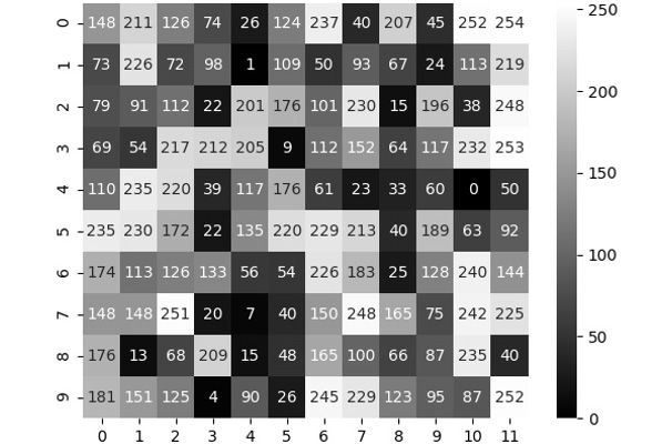
Figure 1.14: Image with pixel values annotated
Now, we know that a grayscale image has only one channel and that's why the pixel value has only one number that determines the shade of color present in that pixel. What if we are talking about an RGB image? Since the RGB image has three channels, each pixel will have three values – one value for the red channel, one for the green channel, and one for the blue channel.Consider the following image, which shows that an RGB image (on the left) is made up of three images or channels – a red channel, a green channel, and a blue channel:

Figure 1.15: RGB image broken down into three channels
What do we know about each of these channels? In Figure 1.11, we saw that each channel image looks exactly like a grayscale image. That's why the pixel value for each channel will range between 0 and 255. What will happen if we assume that the following image has the same pixel values like those shown in Figure 1.14 for the red channel, but the other two channels are zero? Let's have a look at the result:
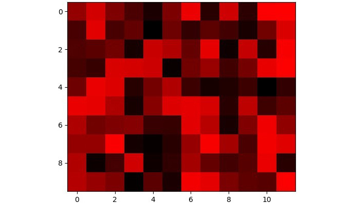
Figure 1.16: RGB image with the red channel set the same as the one used in Figure 1.13
Notice how a 0 for the red channel means that there will be no red color in that pixel. Similarly, a 255-pixel value for the red channel means that there will be a 100% red color in that pixel. By 100% red color, we mean that it won't be some darker shade of red, but the pure (lightest) red color.
Figure 1.17 and Figure 1.18 show the RGB image with a green and a blue channel, respectively. These are the same ones that were shown in Figure 1.14. In each case, we are assuming that the other two channels are zero.
This way, we are highlighting the effect of only one channel:

Figure 1.17: RGB image with the green channel set the same as the one used in Figure 1.14
The output for the blue channel is as follows:
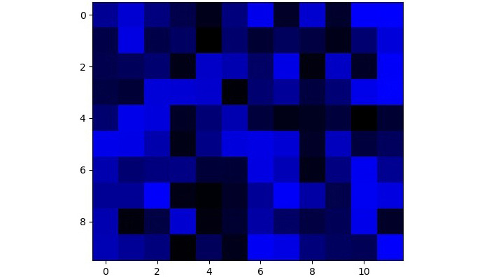
Figure 1.18: RGB image with the blue channel set the same as the one used in Figure 1.14
Now, what will happen if we combine the blue and green frames and keep the red frame set to 0?
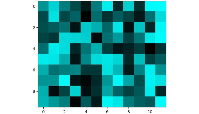
Figure 1.19: RGB image with the blue and green channels set the same as the ones used in Figure 1.14
Notice how the blue and green channels merged to create a shade of cyan. You can see the same shade being formed in the following figure when blue and green are combined:

Figure 1.20: Combination of red, green, and blue
In this section, we discussed the concept of pixel values for grayscale images and images with three channels. We also saw how the pixel value affects the shade of the color present in a specific pixel. So far, we have discussed the important concepts that will be referred to throughout this book. From the next section onward, we will start with coding using various libraries such as OpenCV and Matplotlib.
Introduction to OpenCV
OpenCV, also known as the Open Source Computer Vision library, is the most commonly used computer vision library. Primarily written in C++, it's also commonly used in Python, thanks to its Python wrappers. Over the years, OpenCV has been through multiple revisions and its current version is 4.2.0 (which is the version we are going to use in this book). What makes it different from other computer vision libraries is the fact that it's fast and easy to use, it provides support for libraries such as QT and OpenGL, and most importantly, it provides hardware acceleration for Intel processors. These powerful features/benefits make OpenCV the perfect choice for understanding the various concepts of computer vision and implementing them. Apart from OpenCV, we will also use NumPy for some basic computation and Matplotlib for visualization, wherever required.
Note
Refer to the Preface for NumPy and OpenCV installation instructions.
Let's start by understanding how images are represented in OpenCV in Python.
Images in OpenCV
OpenCV has its own class for representing images – cv::Mat. The "Mat" part comes from the term matrix. Now, this should not come as a surprise since images are nothing more than matrices. We already know that every image has three attributes specific to its dimensions – width, height, and the number of channels. We also know that every channel of an image is a collection of pixel values lying between 0 and 255. Notice how the channel of an image starts to look similar to a 2D matrix. So, an image becomes a collection of 2D matrices stacked on top of each other.
Refer to the following diagram for more details:

Figure 1.21: Image as 2D matrices stacked on top of each other
As a quick recap, while using OpenCV in Python, images are represented as NumPy arrays. NumPy is a Python module commonly used for numerical computation. A NumPy array looks like a 2D matrix, as we saw in Exercise 1.01, Creating NumPy Arrays. That's why an RGB image (which has three channels) will look like three 2D NumPy arrays stacked on top of each other.
We have restricted our discussion so far only to 2D arrays (which is good enough for grayscale images), but we know that our RGB images are not like 2D arrays. They not only have a height and a width; they also have one extra dimension – the number of channels in the image. That's why we can refer to RGB images as 3D arrays.
The only difference to the commands we discussed in the NumPy Arrays section is that we now have to add an extra dimension to the shape of the NumPy arrays – the number of channels. Since we know that RGB images have only three channels, the shape of the NumPy arrays becomes (number of rows, number of columns, 3).
Also, note that the order of elements in the shape of NumPy arrays follows this format: (number of rows, number of columns, 3). Here, the number of rows is equivalent to the height of the image, while the number of columns is equivalent to the width of the image. That's why the shape of the NumPy array can also be represented as (height, width, 3).
Now that we know about how images are represented in OpenCV, let's go ahead and learn about some functions in OpenCV that we will commonly use.
Important OpenCV Functions
We can divide the OpenCV functions that we are going to use into the following categories:
- Reading an image
- Modifying an image
- Displaying an image
- Saving an image
Let's start with the function required for reading an image. The only function we will use for this is cv2.imread. This function takes the following arguments:
- File name of the image we want to read/load
- Flags for specifying what mode we want to read the image in
If we try to load an image that does not exist, the function returns None. This can be used to check whether the image was read successfully or not.
Currently, OpenCV supports formats such as .bmp, .jpeg, .jpg, .png, .tiff, and .tif. For the entire list of formats, you can refer to the documentation: https://docs.opencv.org/4.2.0/d4/da8/group__imgcodecs.html#ga288b8b3da0892bd651fce07b3bbd3a56.
The last thing that we need to focus on regarding the cv2.imread function is the flag. There are only three flags that are commonly used for reading an image in a specific mode:
- cv2.IMREAD_UNCHANGED: Reading the image as it is. This means that if an image is a PNG image with a transparent background, then it will be read as a BGRA image, where A specifies the alpha channel – which is responsible for transparency. If this flag is not used, the image will be read as a BGR image. Note that BGR refers to the blue, green, and red channels of an image. A, or the alpha channel, is responsible for transparency. That's why an image with a transparent background will be read as BGRA and not as BGR. It's also important to note here that OpenCV, by default, uses BGR mode and that's why we are discussing BGRA mode and not RGBA mode here.
- cv2.IMREAD_GRAYSCALE: Reading the image in grayscale format. This converts any color image into grayscale.
- cv2.IMREAD_COLOR: This is the default flag and it reads any image as a color image (BGR mode).
Note
Note that OpenCV reads images in BGR mode rather than RGB mode. This means that the order of channels becomes blue, green, and red. Even with the other OpenCV functions that we will use, it is assumed that the image is in BGR mode.
Next, let's have a look at some functions we can use to modify an image. We will specifically discuss the functions for the following tasks:
- Converting an image's color space
- Splitting an image into various channels
- Merging channels to form an image
Let's learn how we can convert the color space of an image. For this, we will use the cv2.cvtColor function. This function takes two inputs:
- The image we want to convert
- The color conversion flag, which looks as follows:
cv2.COLOR_{CURRENT_COLOR_SPACE}2{NEW_COLOR_SPACE}
For example, to convert a BGR image into an HSV image, you will use cv2.COLOR_BGR2HSV. For converting a BGR image into grayscale, you will use cv2.COLOR_BGR2GRAY, and so on. You can view the entire list of such flags here: https://docs.opencv.org/4.2.0/d8/d01/group__imgproc__color__conversions.html.
Now, let's look at splitting and merging channels. Suppose you only want to modify the red channel of an image; you can first split the three channels (blue, green, and red), modify the red channel, and then merge the three channels again. Let's see how we can use OpenCV functions to split and merge channels:
- For splitting the channels, we can use the cv2.split function. It takes only one argument – the image to be split – and returns the list of three channels – blue, green, and red.
- For merging the channels, we can use the cv2.merge function. It takes only one argument – a set consisting of the three channels (blue, green, and red) – and returns the merged image.
Next, let's look at the functions we will use for displaying an image. There are three main functions that we will be using for display purposes:
- To display an image, we will use the cv2.imshow function. It takes two arguments. The first argument is a string, which is the name of the window in which we are going to display the image. The second argument is the image that we want to display.
- After the cv2.imshow function is called, we use the cv2.waitKey function. This function specifies how long the control should stay on the window. If you want to move to the next piece of code after the user presses a key, you can provide 0. Otherwise, you can provide a number that specifies the number of milliseconds the program will wait before moving to the next piece of code. For example, if you want to wait for 10 milliseconds before moving to the next piece of code, you can use cv2.waitKey(10).
- Without calling the cv2.waitKey function, the display window won't be visible properly. But after moving to the next code, the window will still stay open (but will appear as if it's not responding). To close all the display windows, we can use the cv2.destroyAllWindows() function. It takes no arguments. It's recommended to close the display windows once they are no longer needed.
Finally, to save an image, we will use OpenCV's cv2.imwrite function. It takes two arguments:
- A string that specifies the filename that we want to save the image with
- The image that we want to save
Now that we know about the OpenCV functions that we are going to use in this chapter, let's get our hands dirty by using them in the next exercise.
Exercise 1.02: Reading, Processing, and Writing an Image
In this exercise, we will use the OpenCV functions that we looked at in the previous section to load the image of the lion in Figure 1.3, separate the red, green, and blue channels, display them, and finally save the three channels to disk.
Note
The image can be found at https://packt.live/2YOyQSv.
Follow these steps to complete this exercise:
- First of all, we will create a new notebook – Exercise1.02.ipynb. We will be writing our code in this notebook.
- Let's import the OpenCV module:
import cv2
- Next, let's read the image of the lion and the girl. The image is present at the ../data/lion.jpg path:
Note
Before proceeding, ensure that you can change the path to the image (highlighted) based on where the image is saved in your system.
# Load image
img = cv2.imread("../data/lion.jpg")
Note
The # symbol in the preceding code snippet denotes a code comment. Comments are added into code to help explain specific bits of logic.
- We will check whether we have read the image successfully or not by checking whether it is None:
if img is None:
print("Image not found")
- Next, let's display the image we have just read:
# Display the image
cv2.imshow("Lion",img)
cv2.waitKey(0)
cv2.destroyAllWindows()
The output is as follows:
Note
Please note that whenever we are going to display an image using the cv2.imshow function, a new display window will pop up. This output will not be visible in the Jupyter Notebook and will be displayed in a separate window, as shown in the following figure.
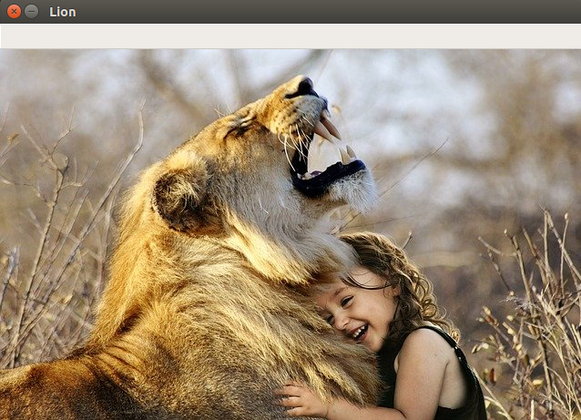
Figure 1.22: Lion image
- Now comes the processing step, where we will split the image into the three channels – blue, green, and red:
# Split channels
blue, green, red = cv2.split(img)
- Next, we can display the channels that we obtained in the preceding step. Let's start by displaying the blue channel:
cv2.imshow("Blue",blue)
cv2.waitKey(0)
cv2.destroyAllWindows()
The output is as follows:
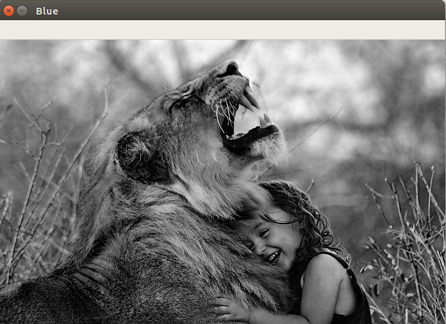
Figure 1.23: Lion image (blue channel)
- Next, let's display the green channel:
cv2.imshow("Green",green)
cv2.waitKey(0)
cv2.destroyAllWindows()
The output is as follows:

Figure 1.24: Lion image (green channel)
- Similarly, we can display the red channel of the image:
cv2.imshow("Red",red)
cv2.waitKey(0)
cv2.destroyAllWindows()
The output is as follows:
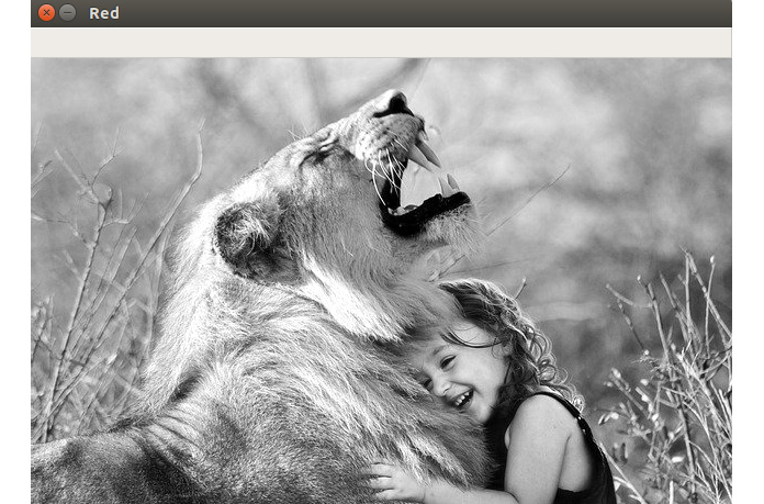
Figure 1.25: Lion image (red channel)
- Finally, to save the three channels we obtained, we will use the cv2.imwrite function:
cv2.imwrite("Blue.png",blue)
cv2.imwrite("Green.png",green)
cv2.imwrite("Red.png",red)
This will return True. This indicates that the images have been successfully written/saved on the disk. At this point, you can verify whether the three channels you have obtained match the images shown here:

Figure 1.26: Blue, green, and red channels obtained using our code
Note
To access the source code for this specific section, please refer to https://packt.live/2YQlDbU.
In the next section, we will discuss another library that is commonly used in computer vision – Matplotlib.
Using Matplotlib to Display Images
Matplotlib is a library that is commonly used in data science and computer vision for visualization purposes. The beauty of this library lies in the fact that it's very powerful and still very easy to use, similar to the OpenCV library.
In this section, we will have a look at how we can use Matplotlib to display images that have been read or processed using OpenCV. The only point that you need to keep in mind is that Matplotlib assumes the images will be in RGB mode, whereas OpenCV assumes the images will be in BGR mode. That's why we will be converting the image to RGB mode whenever we want to display it using Matplotlib.
There are two common ways to convert a BGR image into an RGB image:
- Using OpenCV's cv2.cvtColor function and passing the cv2.COLOR_BGR2RGB flag. Let's imagine that we have an image loaded as img that we want to convert into RGB mode from BGR mode. This can be done using cv2.cvtColor(img, cv2.COLOR_BGR2RGB).
- The second method focuses on the fact that you are reversing the order of channels when you are converting a BGR image into an RGB image. This can be done by replacing img with img[:,:,::-1], where ::-1 in the last position is responsible for reversing the order of channels. We will be using this approach whenever we are displaying images using Matplotlib. The only reason behind doing this is that less time is required to write this code compared to option 1.
Now, let's have a look at the functions we are going to use to display images using Matplotlib.
First, we will import the matplotlib library, as follows. We will be using Matplotlib's pyplot module to create plots and display images:
import matplotlib.pyplot as plt
We will also be using the following magic command so that the images are displayed inside the notebook rather than in a new display window:
%matplotlib inline
Next, if we want to display a color image, we will use the following command, where we are also converting the image from BGR into RGB. We are using the same lion image as before and have loaded it as img:
plt.imshow(img[::-1])
Note
Execute this code in the same Jupyter Notebook where you executed Exercise 1.02, Reading, Processing, and Writing an Image.
The code is as follows:
plt.imshow(img[::-1])
Finally, to display the image, we will use the plt.show() command.
This will give us the following output:
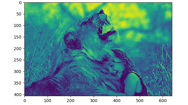
Figure 1.27: Lion image
If we want to display a grayscale image, we will also have to specify the colormap as gray. This is simply because Matplotlib displays grayscale images with a colormap of jet. You can see the difference between the two colormaps in the following plot:
plt.imshow(img, cmap="gray")
The plot looks as follows:
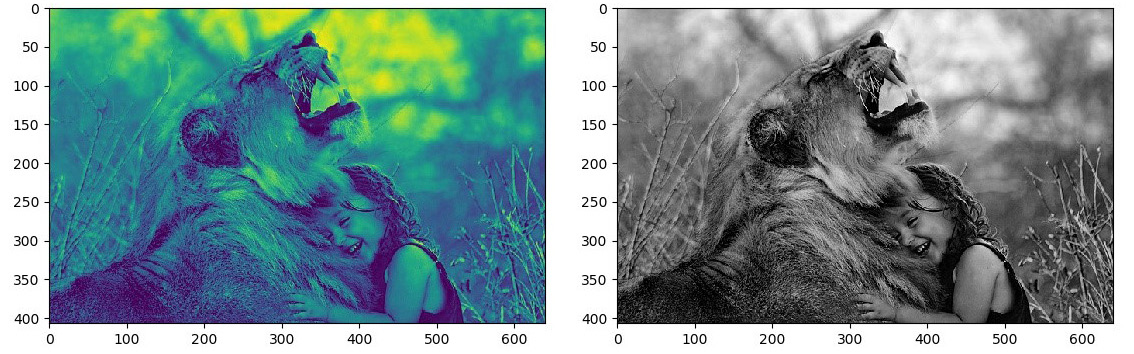
Figure 1.28: (Left) Image without colormap specified, (right) image with a gray colormap
Note
It's very important to note that when we display an image using Matplotlib, it will be displayed inside the notebook, whereas an image displayed using OpenCV's cv2.imshow function will be displayed in a separate window. Moreover, an image displayed using Matplotlib will have the gridlines or X and Y axes, by default. The same will not be present in an image displayed using the cv2.imshow function. This is because Matplotlib is actually a (graph) plotting library, and that's why it displays the axes, whereas OpenCV is a computer vision library. The axes don't hold much importance in computer vision. Please note that irrespective of the presence or absence of the axes, the image graphic will stay the same, whether it's displayed using Matplotlib or OpenCV. That's why any and all image processing steps will also stay the same. We will be using Matplotlib and OpenCV interchangeably in this book to display images. This means that sometimes you will find images with axes and sometimes without axes. In both cases, the axes don't hold any importance and can be ignored.
That's all it takes to display an image using Matplotlib in a Jupyter Notebook. In the next section, we will cover the final topic of this chapter – how to access and manipulate the pixels of an image.
Accessing and Manipulating Pixels
So far, we have discussed how to use OpenCV to read and process an image. But the image processing guide that we have covered so far was very basic and only constituted splitting and merging the channels of an image. Now, let's learn how to access and manipulate pixels, the building blocks of an image.
We can access and manipulate pixels based on their location. We'll learn how we can use the pixel locations in this section.
We already have covered how pixels are located using the coordinate system of an image. We also know that images in OpenCV in Python are represented as NumPy arrays. That's why the problem of accessing pixels becomes the general problem of accessing the elements of a NumPy array.
Let's consider a NumPy array, A, with m rows and n columns. If we want to access the elements present in row number i and column number j, we can do that using A[i][j] or A[i,j].
Similarly, if we want to extract the elements of a NumPy array, A, within rows a and b and columns c and d, we can do that using A[a:b][c:d].
What if we wanted to extract the entire ith row of the array, A? We can do that using A[i][:], where : is used when we want to extract the entire range of elements in that list.
Similarly, if we want to extract the entire jth column, we can use A[:][j].
Manipulating pixels becomes very easy once you have managed to access the pixels you want. You can either change their values to a new value or copy the values from another pixel.
Let's learn how to use the preceding operations by completing a practical exercise.
Exercise 1.03: Creating a Water Effect
In this exercise, we will implement a water filter that is responsible for vertically flipping an object that is floating on a body of water. You can see this effect in the following image:

Figure 1.29: Water effect
The entire problem can be broken down into the following steps:
- Read an image.
- Flip the image vertically.
- Join the original image and the flipped image.
- Display and save the final image.
In this exercise, we will create a water effect using the concepts we have studied so far. We will be applying the same water effect to the lion.jpg image (Figure 1.3) we used earlier. Follow these steps to complete this exercise:
Note
The image can be found at https://packt.live/2YOyQSv.
- Import the required libraries – Matplotlib, NumPy, and OpenCV:
import cv2
import numpy as np
import matplotlib.pyplot as plt
- We will also use the magic command to display images using Matplotlib in the notebook:
%matplotlib inline
- Next, let's read the image and display it. The image is stored in the ../data/lion.jpg path:
Note
Before proceeding, ensure that you can change the path to the image (highlighted) based on where the image is saved in your system.
# Read the image
img = cv2.imread("../data/lion.jpg")
# Display the image
plt.imshow(img[:,:,::-1])
plt.show()
The output is as follows:
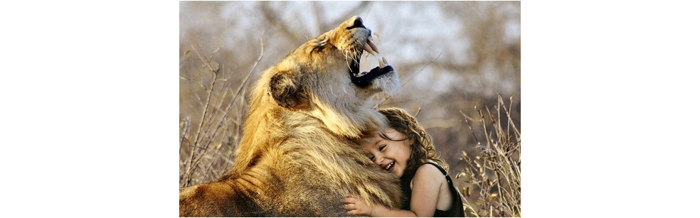
Figure 1.30: Image output
- Let's find the shape of the image to understand what we are dealing with here:
# Find the shape of the image
img.shape
The shape of the image is (407, 640, 3).
- Now comes the important part. We will have to create a new image with twice the number of rows (or twice the height) but the same number of columns (or width) and the same number of channels. This is because we want to add the mirrored image to the bottom of the image:
# Create a new array with double the size
# Height will become twice
# Width and number of channels will
# stay the same
imgNew = np.zeros((814,640,3),dtype=np.uint8)
- Let's display this new image we created. It should be a completely black image at this point:
# Display the image
plt.imshow(imgNew[:,:,::-1])
plt.show()
The output is as follows:

Figure 1.31: New black image that we have created using np.zeros
- Next, we will copy the original image to the top half of the image. The top half of the image corresponds to the first half of the rows of the new image:
# Copy the original image to the
# top half of the new image
imgNew[:407][:] = img
- Let's look at the new image now:
# Display the image
plt.imshow(imgNew[:,:,::-1])
plt.show()
Here's the output of the show() method:

Figure 1.32: Image after copying the top half of the image
- Next, let's vertically flip the original image. We can take some inspiration from how we reversed the channels using ::-1 in the last position. Since flipping the image vertically is equivalent to reversing the order of rows in the image, we will use ::-1 in the first position:
# Invert the image
imgInverted = img[::-1,:,:]
- Display the inverted image, as follows:
# Display the image
plt.imshow(imgInverted[:,:,::-1])
plt.show()
The inverted image looks as follows:

Figure 1.33: Image obtained after vertically flipping the original image
- Now that we have the flipped image, all we have to do is copy this flipped image to the bottom half of the new image:
# Copy the inverted image to the
# bottom half of the new image
imgNew[407:][:] = imgInverted
- Display the new image, as follows:
# Display the image
plt.imshow(imgNew[:,:,::-1])
plt.show()
The output is as follows:

Figure 1.34: Water effect
- Let's save the image that we have just created:
# Save the image
cv2.imwrite("WaterEffect.png",imgNew)
In this exercise, you saw how the toughest-looking tasks can sometimes be completed using the very basics of a topic. Using our basic knowledge of NumPy arrays, we were able to generate a very beautiful-looking image.
Note
To access the source code for this specific section, please refer to https://packt.live/2VC7QDL.
Let's test what we have learned so far by completing the following activity, where we will create a mirror effect. One difference between the water effect and the mirror effect image will be that the mirror effect will be laterally inverted. Moreover, we will also be introducing an additional negative effect to the mirror image. This negative effect gets its name from the image negatives that are used while processing photographs. You can see the effect of the mirror image by looking at the following figure.
Let's test what we have learned so far with the following activity.
Activity 1.01: Mirror Effect with a Twist
Creating a very simple mirror effect is very simple, so let's bring a twist to this. We want to replicate the effect shown in the following figure. These effects are useful when we want to create apps such as Snapchat, Instagram, and so on. For example, the water effect, the mirror effect, and so on are quite commonly used as filters. We covered the water effect in the previous exercise. Now, we will create a mirror effect:

Figure 1.35: Mirror effect
Before you read the detailed instructions, think about how you would create such an effect. Notice the symmetry in the image, that is, the mirror effect. The most important part of this activity is to generate the image on the right. Let's learn how we can do that. We will be using the same image of the lion and girl that we used in the previous exercises.
Note
The image can be found at https://packt.live/2YOyQSv.
Follow these steps to complete this activity:
- First, load the required modules – OpenCV, Matplotlib, and NumPy.
- Next, write the magic command to display the images in the notebook.
- Now, load the image and display it using Matplotlib.
- Next, obtain the shape of the image.
- Now comes the most interesting part. Convert the image's color space from BGR into HSV and display the HSV image. The image will look as follows:
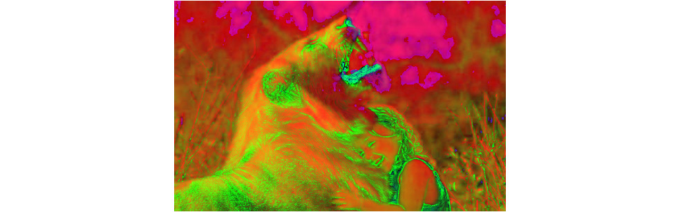
Figure 1.36: Image converted into the HSV color space
- Next, extract the value channel from the HSV color space. Note that the value channel is the last channel of the HSV image. You can use the cv2.split function for this. Display the value channel. The image will look as follows:

Figure 1.37: Value channel of the HSV image
- Now comes another interesting part. We will create a negative effect on the image. This is similar to what you see in the negatives of the images you click. To carry out this effect, all you have to do is subtract the value channel from 255. Then, display the new value channel. The image will look as follows:
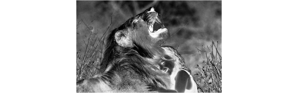
Figure 1.38: Negative of the value channel
- Next, create a new image by merging the value channel with itself. This can be done by using cv2.merge((value, value, value)), where value refers to the negative of the value channel you obtained in the preceding step. We are doing this because we want to merge two three-channel images to create the final effect.
- Next, flip the new image you obtained previously, horizontally. You can refer to the flipping step we did in Exercise 1.03, Creating a Water Effect. Note that flipping horizontally is equivalent to reversing the order of the columns of an image. The output will be as follows:
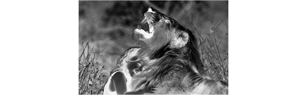
Figure 1.39: Image flipped horizontally
- Now, create a new image with twice the width as the original image. This means that the number of rows and the number of channels will stay the same. Only the number of columns will be doubled.
- Now, copy the original image to the left half of the new image. The image will look as follows:
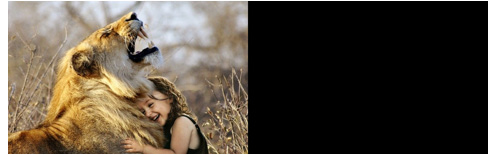
Figure 1.40: Copying the original image to the left half
- Next, copy the horizontally flipped image to the right half of the new image and display the image.
- Finally, save the image you have obtained.
The final image will look as follows:
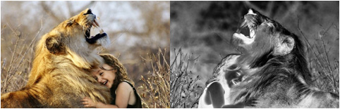
Figure 1.41: Final image
Note
The solution to this activity can be found on page 466.
In this activity, you used the concepts you studied in the previous exercise to generate a really interesting result. By completing this activity, you have learned how to convert the color space of an image and use a specific channel of the new image to create a mirror effect.
Summary
This brings us to the end of the first chapter of this book. We started by discussing the important core concepts of computer vision – what an image is, what pixels are, and what their attributes are. Then, we discussed the libraries that we will use throughout our computer vision journey – OpenCV, Matplotlib, and NumPy. We also learned how we can use these libraries to read, process, display, and save images. Finally, we learned how to access and manipulate pixels and used this concept to generate interesting results in the final exercise and activity.
In the next chapter, we will look deeper into image processing and how OpenCV can help us with that. The more you practice, the easier it will be for you to figure out what concept you need to employ to get a result. So, keep on practicing.