
15
CHAPTER
Impedance and Admittance
IN THIS CHAPTER, WE’LL DEVELOP A “RIGOROUS” WORKING MATHEMATICAL MODEL FOR COMPLEX impedance. We’ll also learn about admittance, which quantifies how well AC circuits allow (or admit) the flow of current, rather than restraining (or impeding) it.
Imaginary Numbers Revisited
As we learned in Chap. 13, the engineering symbol j represents the unit imaginary number, technically defined as the positive square root of −1. Let’s review this concept, because some people find it difficult to believe that negative numbers can have square roots. When we multiply j by itself, we get −1.
The term “imaginary” comes from the notion that j is somehow “less real” than the so-called real numbers. That’s not true! All numbers are “unreal” in the sense that they’re all abstract, however we classify them. You know that, if you’ve ever taken a course in number theory.
Actually, j isn’t the “only” square root of −1. A negative square root of −1 also exists; it equals −j. When we multiply either j or −j by itself, we get −1. (Pure mathematicians often denote these same numbers as i or −i.) The set of imaginary numbers comprises all possible real-number multiples of j. Examples include:
• j × 4, which we write as j4
• j × 35.79, which we write as j35.79
• j × (−25.76), which we write as −j25.76
• j × (−25,000), which we write as −j25,000
We can multiply j by any real number and portray it as a point on a line. If we do that for all the real numbers, we get an imaginary-number line (Fig. 15-1). We orient the imaginary number line vertically, at a right angle to the horizontal real number line, when we want to graphically render real and imaginary numbers at the same time. In electronics, real numbers represent resistances. Imaginary numbers represent reactances.

15-1 The imaginary-number line.
Complex Numbers Revisited (in Detail)
When we add a real number and an imaginary number, we get a complex number. In this context, the term “complex” does not mean “complicated”; a better word might be “composite.” Examples include:
• The sum of 4 and j5, which equals 4 + j5
• The sum of 8 and −j7, which equals 8 − j7
• The sum of −7 and j13, which equals −7 + j13
• The sum of −6 and −j87, which equals −6 − j87
To completely portray the set of complex numbers in graphical form, we need a two-dimensional coordinate plane.
Adding and Subtracting Complex Numbers
When we want to add one complex number to another, we add the real parts and the complex parts separately and then sum up the total. For example, the sum of 4 + j7 and 45 − j83 works out as
(4 + 45) + j(7 − 83) = 49 + j(−76) = 49 − j76
Subtracting complex numbers involves a little trickery because we can easily confuse our signs. We can avoid this confusion by converting the difference to a sum. For example, we can find the difference (4 + j7) − (45 − j83) if we first multiply the second complex number by −1 and then add the result, obtaining
(4 + j7) − (45 − j83) = (4 + j7) + [−1(45 − j83)]
= (4 + j7) + (−45 + j83) = [4 + (−45)] + j(7 + 83)
= −41 + j90
Alternatively, you can subtract the real and imaginary parts separately, and then combine the result back into an imaginary number to get your final answer. Subtracting the negative of a quantity is the same as adding that quantity. Working out the above difference without converting to a sum, you’ll get
(4 + j7) − (45 − j83) = (4 − 45) + j[7 − (−83)]
= −41 + j(7 + 83) = −41 + j90
Multiplying Complex Numbers
When we want to multiply one complex number by another, we should treat them both as sums of number pairs—that is, as binomials. If we have four real numbers a, b, c, and d, then
(a + jb) (c + jd) = ac + jad + jbc + j2 bd
= (ac − bd) + j(ad + bc)
The Complex Number Plane
We can construct a complete complex-number plane by taking the real and imaginary number lines and placing them together, at right angles, so that they intersect at the zero points, 0 and j0. Figure 15-2 illustrates the arrangement, which gives us a rectangular coordinate plane, just like the ones that people use to graph everyday relations, such as temperature versus time.

15-2 The complex number plane.
Complex Number Vectors
Engineers sometimes represent complex numbers as vectors in the coordinate plane. This gives each complex number a unique magnitude and a unique direction. The magnitude of the vector for a complex number a + jb equals the distance of the point (a, jb) from the origin (0, j0). We represent the vector direction as the angle, expressed going counterclockwise from the positive real-number axis. Figure 15-3 illustrates how this scheme works.

15-3 Magnitude and direction of a vector in the complex number plane.
Absolute Value
The absolute value of a complex number a + jb equals the length, or magnitude, of its vector in the complex plane, measured from the origin (0, j0) to the point (a, jb). Let’s break this scenario down into three cases.
1. For a pure real number a + j0, the absolute value equals a, if a is positive. If a is negative, the absolute value of a + j0 equals −a.
2. For a pure imaginary number 0 + jb, the absolute value equals b, if b (a real number) is positive. If b is negative, the absolute value of 0 + jb equals −b.
3. If the number a + jb is neither a pure real nor a pure imaginary number, we must use a formula to find its absolute value. First, we square both a and b. Then we add those two squares. Finally, we take the square root of the sum of the squares to get the length c of the vector representing a + jb. Figure 15-4 shows the geometry of this method.

15-4 Calculation of the absolute value (length) of a vector. Here, we represent the vector length as c.
Problem 15-1
Find the absolute value of the complex number –22 – j0.
Solution
We have a pure real number in this case. Actually, –22 – j0 is the very same complex number as –22 + j0, because −j0 = j0. The absolute value equals –(–22), or 22.
Find the absolute value of 0 – j34.
Solution
This quantity is a pure imaginary number where b = –34 because 0 – j34 = 0 + j(–34). The absolute value equals –(–34), or 34.
Problem 15-3
Find the absolute value of 3 – j4.
Solution
In this case, we have a = 3 and b = –4. Using the formula described above and shown in Fig. 15-4, we get
[32 + (–4)2]1/2 = (9 + 16)1/2 = 251/2 = 5
The RX Half-Plane
Recall the quarter-plane for resistance R and inductive reactance XL from Chap. 13. This region corresponds to the upper-right quadrant of the complex number plane shown in Fig. 15-2. Similarly, the quarter-plane for resistance R and capacitive reactance XC corresponds to the lower-right quadrant of the complex number plane of Fig. 15-2. We represent resistances as nonnegative real numbers. We represent reactances as imaginary numbers.
No Negative Resistance
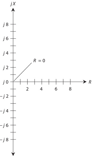
Strictly speaking, negative resistance can’t exist because we can’t have anything better than a perfect conductor. In some cases, we might treat a source of DC, such as a battery, as if it constitutes a “negative resistance.” Once in a while, we might encounter a device in which the current drops as the applied voltage increases, producing a “reversed” resistance-behavior phenomenon that some engineers call “negative resistance.” But for most practical applications, the resistance can never go “below zero.” We can, therefore, remove the negative axis, along with the upper-left and lower-left quadrants, of the complex-number plane, obtaining an RX half-plane, as shown in Fig. 15-5. This system provides a complete set of coordinates for depicting complex impedance.
15-5 The complex impedance half-plane, also called the resistance-reactance (RX) half-plane.
“Negative Inductors” and “Negative Capacitors”
Capacitive reactance XC is effectively an extension of inductive reactance XL into the realm of negatives. Capacitors act like “negative inductors.” We can also say that inductors act like “negative capacitors” because the negative of a negative number equals a positive number. Reactance, in general, can vary from extremely large negative values, through zero, to extremely large positive values.
Complex Impedance Points
Imagine the point representing R + jX moving around in the RX half-plane, and imagine where the corresponding points on the axes lie. We can locate these points by drawing dashed lines from the point R + jX to the R and X axes, so that the dashed lines intersect the axes at right angles. Figure 15-6 shows several examples.

15-6 Some points in the RX half-plane, showing their resistance and reactance components.
Now think of the points for R and X moving toward the right and left, or up and down, on their axes. Imagine what happens to the point representing R + jX in various scenarios. This exercise will give you an idea of how impedance changes as the resistance and reactance vary in an AC electrical circuit.
Resistance constitutes a one-dimensional phenomenon. Reactance also manifests itself as one-dimensional. To completely define complex impedance, however, we must use two dimensions. The RX half-plane meets this requirement. Remember that the resistance and the reactance can vary independently of one another!
Complex Impedance Vectors
We can represent any impedance R + jX as a complex number of the form a + jb. We simply let R = a and X = b. Now we can envision how the impedance vector changes as we vary either the resistance R or the reactance X, or both, independently. If X remains constant, an increase in R causes the complex impedance vector to grow longer. If R remains constant and XL gets larger, the vector grows longer. If R stays the same but XC gets larger negatively, the vector once again grows longer. Figure 15-7 illustrates the vectors corresponding to the points from Fig. 15-6.

15-7 Vectors representing the points shown in Fig. 15-6.
Absolute-Value Impedance
You’ll occasionally read or hear that the “impedance” of some device or component equals a certain number of “ohms.” For example, in audio electronics, you’ll encounter things like “8-ohm” speakers and “600-ohm” amplifier inputs. How, you ask, can manufacturers quote a single number for a quantity that needs two dimensions for its complete expression? That’s a good question. Two answers exist.
First, specifications, such as “8 ohms” for a speaker or “600 ohms” for an amplifier input, refer to purely resistive impedances, also known as non-reactive impedances. Thus, the “8-ohm” speaker really has a complex impedance of 8 + j0, and the “600-ohm” input circuit is designed to operate with a complex impedance at, or near, 600 + j0.
Second, you can talk about the length of the impedance vector (the absolute value of the complex impedance), calling this length a certain number of ohms. If you try to define impedance this way, however, you risk ambiguity and confusion because you can find infinitely many different vectors of a given length in the RX half-plane.
Sometimes, engineers and technicians write the uppercase, italic letter Z in place of the word “impedance,” so you’ll read expressions such as “Z = 50 ohms” or “Z = 300 ohms nonreactive.” In this context, if no specific impedance is given, “Z = 8 ohms” can theoretically refer to 8 + j0, 0 + j8, 0 – j8, or any other complex impedance whose point lies on a half-circle centered at the coordinate origin and having a radius of 8 units, as shown in Fig. 15-8.

15-8 Some vectors representing an absolute-value impedance of 8 ohms. Infinitely many such vectors exist in theory, all of which terminate on the dashed circle.
Problem 15-4
Name seven different complex impedances that the expression “Z = 10 ohms” might mean.
Solution
We can easily name three such impedance values, each consisting of a pure reactance or a pure resistance, as follows:
Z1 = 0 + j10
Z2 = 10 + j0
Z3 = 0 – j10
These impedances represent pure inductance, pure resistance, and pure capacitance, respectively.
A right triangle can exist having sides in a ratio of 6:8:10 units. We know this fact from basic coordinate geometry, because 62 + 82 = 102. Therefore, we can have the following impedances, all of which have an absolute value of “10 ohms”:
Z4 = 6 + j8
Z5 = 6 – j8
Z6 = 8 + j6
Z7 = 8 – j6
Characteristic Impedance
You’ll sometimes encounter a property of certain electrical components known as characteristic impedance or surge impedance, symbolized Zo. Characteristic impedance constitutes a fundamental property of transmission lines.
Transmission-Line Types
Engineers and technicians use transmission lines to get energy or signals from one place to another. We can always express transmission-line Zo values in ohms as positive real numbers. We don’t need complex numbers to define it.
Transmission lines usually take either of two forms, coaxial or two-wire (also called parallel-wire). Figure 15-9 illustrates cross-sectional renditions of both types. Examples of transmission lines include the “ribbon” that goes from an old-fashioned television (TV) antenna to the receiver set, the cable running from a hi-fi amplifier to the speakers, and the set of wires that carries electricity across the countryside.

15-9 Cross-sectional views of coaxial transmission line (A) and parallel-wire transmission line (B).
Figure 15-9A shows a cross-section of a coaxial transmission line. The line has a wire center conductor that runs along a defined axis, and an outer conductor or shield in the shape of a conducting cylinder concentric with that same axis. The value of Zo depends on the radius r1 of the center conductor, on the inside radius r2 of the shield, and on the type of dielectric material separating the center conductor from the shield. If we make the center conductor wire thicker (we increase r1) while leaving all other factors unchanged, then Zo decreases. If we enlarge the cylindrical shield (we increase r2) while leaving all other factors unchanged, then Zo increases.
Figure 15-9B shows a cross-sectional view of a parallel-wire transmission line. The value of Zo depends on the radii r of the wires, on the spacing d between the centers of the wires, and on the nature of the dielectric material separating the wires. In general, the value of Zo increases as the wire radii r get smaller, and decreases as the wire radii get larger, if we hold all other factors constant. (We assume that both wires have the same radius r.) If we leave the wire radii r constant but increase the spacing d between them, then Zo increases. If we bring the wires closer together (decrease d) while leaving their radii r constant, then Zo decreases.
Solid dielectric materials, such as polyethylene, when placed between the conductors, reduce the characteristic impedance of a transmission line, as compared with air or a vacuum. The extent of the reduction depends on the dielectric constant of the material. As we make the dielectric constant larger, while all other parameters remain constant in a transmission line, the extent of the reduction in Zo (compared with air or a vacuum between the conductors) becomes greater.
Zo in Practice
The ideal value of Zo for a transmission line depends on the nature of the load into which the line delivers energy. If the load has a purely resistive impedance of R ohms, the value of the best line Zo equals R ohms. If the load impedance is not a pure resistance, or if it’s a pure resistance that differs considerably from the characteristic impedance of the transmission line, some energy goes to waste in heating up the transmission line. As the so-called impedance mismatch grows worse, the proportion of the energy wasted as heat goes up, and the transmission-line efficiency suffers.
Imagine a so-called “300-ohm” frequency-modulation (FM) receiving antenna, such as the folded-dipole type that you can install indoors. Suppose that you want to obtain the best possible reception. Of course, you should choose a good location for the antenna. You should make sure that the transmission line between your radio and the antenna remains as short as possible. But you should also ensure that you purchase “300-ohm” TV ribbon. The manufacturer of that ribbon has optimized its Zo value for use with antennas whose impedances are close to 300 + j0, representing a pure resistance of 300 ohms without any reactance.
Conductance
In an AC circuit, electrical conductance behaves exactly as it does in a DC circuit. We symbolize conductance (as a variable in equations) by writing an uppercase italic letter G. We express the relationship between conductance and resistance as the two formulas
G = 1/R
and
R = 1/G
The standard unit of conductance is the siemens, abbreviated as the uppercase non-italic letter S. In the above formulas, we get G in siemens if we input R in ohms, and vice-versa. As the conductance increases, the resistance decreases, and more current flows for a fixed applied voltage. Conversely, as G decreases, R goes up, and less current flows when we apply a fixed voltage.
Susceptance
Sometimes we’ll come across the term susceptance in reference to AC circuits. We symbolize this quantity (as a variable in equations) by writing an uppercase italic letter B. Susceptance is the reciprocal of reactance, and it can occur in either the capacitive form or the inductive form. If we symbolize capacitive susceptance as BC and inductive susceptance as BL, then
BC = 1/XC
and
BL = 1/XL
The Reciprocal of j
All values of B theoretically contain the j operator, just as do all values of X. But when it comes to finding reciprocals of quantities containing j, things get tricky. The reciprocal of j actually equals its negative! That is,
1/j = –j
and
1/(–j) = j
As a result of these properties of j, the sign reverses whenever you find a susceptance value in terms of a reactance value. When expressed in terms of j, inductive susceptance is negative imaginary, and capacitive susceptance is positive imaginary—just the opposite situation from inductive reactance and capacitive reactance.
Imagine an inductive reactance of 2 ohms. We express this in imaginary terms as j2. To find the inductive susceptance, we must find 1/(j2). Mathematically, we convert this expression to a real-number multiple of j by breaking it down in steps as follows:
1/(j2) = (1/j)(1/2) = (1/j)0.5 = –j0.5
Now imagine a capacitive reactance of 10 ohms. We express this quantity in imaginary terms as –j10. To find the capacitive susceptance, we must find 1/(–j10). Here’s how we can convert it to the product of j and a real number:
1/(–j10) = (1/–j)(1/10) = (1/–j)0.1 = j0.1
To find an imaginary value of susceptance in terms of an imaginary value of reactance, we must first take the reciprocal of the real-number part of the expression, and then multiply the result by –1.
Problem 15-5
Suppose that we have a capacitor of 100 pF at a frequency of 3.10 MHz. What’s the capacitive susceptance BC?
First, let’s find XC by using the formula for capacitive reactance. We have
XC = –1/(6.2832 fC)
Note that 100 pF = 0. 000100 μF. Therefore
![]()
The imaginary value of XC equals –j513. The susceptance BC equals 1/XC, so we have
BC = 1/(–j513) = j0.00195 S
The siemens quantifies susceptance, just as it defines conductance. Therefore, we can state the foregoing result as 0.00195 S of capacitive susceptance.
General Formula for BC
We can now see that the general formula for capacitive susceptance in siemens, in terms of frequency in hertz and capacitance in farads, is
BC = 6.2832 fC
This formula also works for frequencies in megahertz and capacitance values in microfarads.
Problem 15-6
Suppose an inductor has L = 163 μH at a frequency of 887 kHz. What’s the inductive susceptance BL?
Solution
Note that 887 kHz = 0.887 MHz. We can calculate XL from the formula for inductive reactance as follows:
XL = 6.2832 fL = 6.2832 × 0.887 × 163 = 908 ohms
The imaginary value of XL equals j908. The susceptance BL equals 1/XL. It follows that
BL = –1/(j908) = –j0.00110 S
We can state this result as −0.00110 S of inductive susceptance.
General Formula for BL
The general formula for inductive susceptance in siemens, in terms of frequency in hertz and inductance in henrys, is
BL = –1/(6.2832 fL)
This formula also works for frequencies in kilohertz and inductance values in millihenrys, and for frequencies in megahertz and inductance values in microhenrys.
Admittance
Real-number conductance and imaginary-number susceptance combine to form complex admittance, symbolized (as a variable in equations) as the uppercase italic letter Y. Admittance provides a complete expression of the extent to which a circuit allows AC to flow. As the absolute value of complex impedance gets larger, the absolute value of complex admittance becomes smaller, in general. Huge impedances correspond to tiny admittances, and vice-versa.
Complex Admittance
We can express admittance in complex form, just as we can do with impedance. However, we’d better keep careful track of which quantity we’re talking about! We can avoid confusion if we take care to employ the correct symbol. We can get a complete expression of admittance by taking the complex composite of conductance and susceptance. Engineers usually write complex admittance in the form
Y = G + jB
when the susceptance is positive (capacitive), and in the form
Y = G – jB
when the susceptance is negative (inductive).
The “Parallel Advantage”
In Chaps. 13 and 14, we worked with series RL and RC circuits. Did you wonder, at that time, why we ignored parallel circuits in those discussions? We had a good reason: Admittance works far better than impedance when we want to mathematically analyze parallel AC circuits. In parallel AC circuits, resistance and reactance combine to make a mathematical mess. But conductance and susceptance add directly together in parallel circuits, yielding admittance. We’ll analyze parallel RL and RC circuits in the next chapter.
The GB Half-Plane
We can portray complex admittance on a coordinate grid similar to the complex-impedance (RX) half-plane. We get a half-plane, not a complete plane because no such thing as negative conductance exists in the “real world.” (We can’t have a component that conducts worse than not at all!) We plot conductance values along a horizontal G axis. We plot susceptance along a vertical B axis. Figure 15-10 shows several points on the GB half-plane.

15-10 Some points in the GB half-plane, along with their conductance and susceptance components.
It’s Inside-Out
Superficially, the GB half-plane looks identical to the RX half-plane. But mathematically, the two couldn’t differ more! The GB half-plane is “inside-out” with respect to the RX half-plane. The center, or origin, of the GB half-plane represents the point at which no conductance exists for DC or for AC. It represents the zero-admittance point rather than the zero-impedance point. In the GB half-plane, the origin corresponds to a perfect open circuit. In the RX half-plane, the origin represents a perfect short circuit.
As you move out toward the right (“east”) along the G, or conductance, axis of the GB half-plane, the conductance improves, and the current gets greater. When you move upward (“north”) along the jB axis from the origin, you have ever-increasing positive (capacitive) susceptance. When you go downward (“south”) along the jB axis from the origin, you encounter increasingly negative (inductive) susceptance.
Vector Representation of Admittance
We can denote specific complex admittance values as vectors, just as we can do with complex impedance values. Figure 15-11 shows the points from Fig. 15-10 as complex admittance vectors. Given a fixed applied AC voltage, long vectors in the GB half-plane generally indicate large currents, and short vectors indicate small currents.

15-11 Vectors representing the points shown in Fig. 15-10.
Imagine a point moving around on the GB half-plane. Think of the vector getting longer and shorter, and changing direction as well. Vectors pointing generally “northeast,” or upward and to the right, correspond to conductances and capacitances in parallel. Vectors pointing in a more or less “southeasterly” direction, or downward and to the right, portray conductances and inductances in parallel.
Quiz
Refer to the text in this chapter if necessary. A good score is 18 or more correct. Answers are in the back of the book.
1. The positive square root of a negative real number equals
(a) a smaller real number.
(b) a larger real number.
(c) a positive real-number multiple of the j operator.
(d) 0.
2. The reciprocal of the j operator equals
(a) itself.
(b) its negative.
(c) a real number.
(d) 0.
3. If we add a real number to an imaginary number, we get
(a) a real number.
(b) an imaginary number.
(c) a complex number.
(d) −1.
4. What’s the sum (−1 + j7) + (3 − j5)?
(a) 2 + j2
(b) 2 − j2
(c) −2 + j2
(d) −2 − j2
5. What’s the sum (3 − j5) + (−1 + j7)?
(a) 2 + j2
(b) 2 − j2
(c) −2 + j2
(d) −2 − j2
6. What’s the difference (−1 + j7) − (3 − j5)?
(a) 4 + j12
(b) 4 − j12
(c) −4 + j12
(d) −4 − j12
7. What’s the difference (3 − j5) − (−1 + j7)?
(a) 4 + j12
(b) 4 − j12
(d) −4 − j12
8. If a specification paper tells you that a certain device has a nominal output impedance of “50 ohms,” the manufacturer means that the load should ideally exhibit a complex impedance of
(a) 50 + j50.
(b) 50 + j50 or 50 − j50.
(c) 0 + j50 or 0 − j50.
(d) None of the above
9. The complex impedance value 15 + j15 could represent
(a) a pure resistance.
(b) a pure reactance.
(c) a resistor in series with an inductor.
(d) a resistor in series with a capacitor.
10. Which, if any, of the following complex numbers has an absolute value of 25?
(a) 15 − j20
(b) 12.5 − j12.5
(c) 5 − j5
(d) None of the above
11. What’s the absolute-value impedance of 4.50 + j5.50?
(a) 4.50 ohms
(b) 5.50 ohms
(c) 7.11 ohms
(d) 50.5 ohms
12. What’s the absolute-value impedance of 0.0 − j36?
(a) 0.0 ohms
(b) 6.0 ohms
(c) 18 ohms
(d) 36 ohms
13. What’s the magnitude of the vector whose end point lies at (1000,−j1000) on the complex-number plane?
(a) 1000
(b) 1414
(c) 2000
(d) 2828
14. What’s the magnitude of the vector whose end point lies at (−1000,−j1000) on the complex-number plane?
(a) 1000
(b) 1414
(c) 2000
(d) 2828
15. If we enlarge the inside radius of the shield of a coaxial cable but don’t change anything else about the cable, what happens to its characteristic impedance?
(a) It increases.
(b) It does not change.
(c) It decreases.
(d) We need more information to answer this question.
16. If we increase the radii of both wires in a two-wire transmission line but don’t change anything else about the line, what happens to its characteristic impedance?
(a) We need more information to answer this question.
(b) It increases.
(c) It does not change.
(d) It decreases.
17. Suppose that a capacitor has a value of 0.010 μF at 1.2 MHz. What’s the capacitive susceptance, stated as an imaginary number?
(a) BC = j0.075
(b) BC = −j0.075
(c) BC = j13
(d) BC = −j13
18. Absolute-value impedance equals the square root of
(a) the real-number coefficient of the reactance plus the imaginary-number part of the admittance.
(b) the real-number resistance plus the real-number coefficient of the reactance.
(c) the real-number conductance plus the real-number coefficient of the susceptance.
(d) None of the above
19. Suppose that an inductor has a value of 10.0 mH at 15.91 kHz. What’s the inductive susceptance, stated as an imaginary number?
(a) BL = −j1000
(b) BL = j1000
(c) BL = −j0.00100
(d) BL = j0.00100
20. When we add the reciprocal of real-number resistance to the reciprocal of imaginary-number reactance, we get complex-number
(a) impedance.
(b) conductance.
(c) susceptance.
(d) admittance.