
4 Direct Normal Irradiance
We receive from the sun perfectly enormous quantities of radiation.
Charles Greeley Abbot
(1872–1973)
4.1 Overview of Direct Normal Irradiance
Solar radiation that arrives at the earth’s surface having come directly from the sun is defined as direct normal irradiance (DNI). Even if the sky is clear, DNI is smaller than would be measured at the top of the earth’s atmosphere because DNI has undergone scattering (by molecules and aerosols) and absorption (by gases and aerosols) within the earth’s atmosphere If clouds are between the sun and the observer, and they are optically thick, then no direct normal irradiance reaches the earth’s surface. The global horizontal irradiance (GHI) observed at the surface is a mixture of DNI that reaches the earth’s surface without being scattered or absorbed and diffuse horizontal irradiance (DHI), the irradiance resulting from molecules, aerosols, and clouds scattering of the DNI. This partitioning is ever changing because the atmosphere is not static. The governing equation is
where sza is the solar zenith angle, the angle between the zenith and solar directions. This partitioning is illustrated in Figure 4.1. It is easy to see that the solid dark line GHI is the sum of the direct normal component on the horizontal in gray (the first term in Equation 4.1) plus the dotted line DHI (the second term of the equation). This is consistent throughout the day until the sun is completely blocked and the first term on the right-hand side in Equation 4.1 goes to zero, leaving GHI equal to DHI between 16:00 and 17:00 and after 17:30 where the solid dark line and the dotted line coincide.
The sun’s output at the top of the earth’s atmosphere, called the total solar irradiance (TSI), has been measured by a variety of space-based radiometers over several decades. The latest is the total irradiance monitor (TIM) on the SOlar Radiation and Climate Experiment (SORCE) satellite (http://lasp.colorado.edu/sorce). TIM measurements of the TSI began in March 2003 and indicate stable solar output with the largest variation of around 0. 3%, lasting just a few days, but with typical variations of TSI under 0.1% (Kopp and Lean, 2011). The sun’s output is so stable that it goes by the misnomer “solar constant.” Even this almost constant value at the top of the earth’s atmosphere changes for the simple reason that the distance between the sun and the earth changes as explained in Chapter 2 The earth’s orbit around the sun causes a change in the amount of solar radiation received at the top of the earth’s atmosphere by a little over 6 .7% between early January when it has its highest value (minimum earth-sun distance) and early July when it has its lowest value (maximum earth-sun distance). This change is entirely predictable from simple orbital mechanics and must be taken into account when computing the extraterrestrial radiation (ETR).

FIGURE 4.1 A demonstration of the partitioning of the GHI into the horizontal component of DNI and DHI using actual data from NREL’s Solar Radiation Research Laboratory. DNI can be higher than GHI when it is clear (dashed). When it is cloudy, GHI is equal to DHI (e. g., between 16:00 and 17:00).
The amount of direct solar radiation that reaches the earth’s surface is much more uncertain and difficult to forecast. Direct normal (“beam”) irradiance is the only form of sunlight that can be used for concentrating solar energy conversion technologies such as concentrating solar power (CSP) thermal systems, which produce steam to generate electricity, and concentrating photovoltaic (CPV), which generate electricity directly. Flat plate collectors such as those that heat water and flat photovoltaic modules that produce electricity, often on the roofs of houses or businesses, can use any incident solar radiation: direct sunlight, sunlight that has been scattered by clouds, molecules, aerosols in the atmosphere, or sunlight reflected by the surface. DNI plays an important role for solar flat plate collectors because it offers the highest energy density for conversion. As shown in Figure 4.2, the area under the DNI time-series curve can represent the largest amount of solar energy available for a day Flat plate solar collectors can be mounted with a fixed, adjustable, or tracking mode for optimum energy conversion. Under clear and partly cloudy sky conditions, DNI often is the predominant contributor to the plane of array (POA) solar irradiance.
Measuring DNI costs the most in the field of broadband solar and infrared radiation measurement Although a good pyrheliometer for measuring DNI is typically less expensive than a good pyranometer used to measure GHI, the pyrheliometer must be accurately pointed at the sun from sunrise to sunset. Good automatic solar trackers are much more costly than the typical thermopile pyrheliometer, usually 5 to 10 times higher. Less expensive clock-drive trackers have been used but require regular adjustments to keep the pyrheliometer pointed at the sun. Because of expense or the requirement to regularly align a manual tracker, there are relatively few continuous, long-term measurements of DNI with a pyrheliometer mounted on an automatic solar tracker. Globally, there are perhaps 100 times more pyranometer installations measuring GHI than pyrheliometers measuring DNI (http://www.nrel.gov/rredc/pdfs/solar_inventory.pdf; Stoffel et al., 2010). However, long-term direct beam data are crucial for selecting a CSP or CPV site, for estimating the expected annual output from a functioning plant, and for developing an operating strategy for the solar plant Given the millions of dollars in capital costs to establish a large solar power plant, it is surprising that a reliable pyrheliometer and tracker are not used more often in prospecting for appropriate sites. Once operations begin, direct beam data are useful to estimate the plant’s efficiency and to spot problems with plant operations. Although surface measurements are the most accurate, it is reasonable to use DNI estimated from satellite images to make initial surveys of the direct solar resource (Vignola, Harlan, Perez, and Kmiecik, 2005). Satellites can prospect over a wide area, and analysis of these satellite-based surveys can help narrow the search for the optimum CSP or CPV location in an area. When anchored by accurate ground-based data from the same general area, systematic errors in the satellite estimates can be accurately assessed and a more precise determination of the solar resource can be made Another advantage of satellite estimates is that geostationary satellites have been flying for decades, so even a year’s worth of surface-based data can be used to validate satellite-estimated irradiance Satellite-derived estimates can then be used to evaluate the interannual variability and long-term trends of solar radiation at the site Again, ground-based measurements can be used to reduce biases in the satellite-derived estimates. Further, satellites in combination with ground-based measurements will find increasing use in short-term forecasting of the solar resource. DNI data from both sources will be an indispensable aid in future solar energy power plant operation, allowing plant operators to optimize the integration of renewables into a utility’s electrical grid. As renewable energy systems increase their contribution to the electrical energy mix in the United States, the transmission of solar-generated electricity from geographically dispersed solar power generators needs to be managed with accurate solar forecast information.
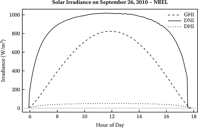
FIGURE 4.2 Demonstration of the integrated DNI far exceeding the integrated GHI on a very clear day.
An alternative to pointing a pyrheliometer at the sun is the concept of the rotating shadowband radiometer (RSR). Chapter 7 describes two types of RSRs in detail, but we discuss this instrument here because it is another method to obtain the DNI, although, necessarily, with some loss of accuracy. Figure 3.21 is from Wesely (1982), and it shows a simple implementation of the RSR and is the first description of such an instrument known to the authors. The pyranometer was a Lambda (now LI-COR model 200) silicon photodiode instrument with a very fast (∼10 μ.sec) time constant The shade band axis is pointed south in a northern hemisphere deployment, and it is rotated with constant speed When the band is beneath the motor housing, a measurement is made of the GHI, and with the LI-COR diffuser completely shaded by the band in front of the sun, a measurement is made of the DHI If the skies are clear and stable, the difference of these two measurements is the horizontal component of the DNI that would fall on this pyranometer. The DNI can be obtained by dividing by cos (sza) If the cosine response of the LI-200 pyranometer is measured, a correction for the imperfect cosine response can be made to further improve the results Other factors that add to the estimated DNI uncertainty include the temperature dependence of the photodiode pyranometer; the spectral response of silicon, which is neither flat nor responsive over the whole solar spectrum; and the need to correct for excess diffuse skylight blocked by the relatively wide band With these corrections properly made, a reasonable estimate of DNI can be obtained, although it will be inferior to a good tracking pyrheliometer This instrument eliminates the necessity of an expensive tracker, but, as will be shown in Chapter 7, it requires considerable effort to correct the results.
4.2 Pyrheliometer Geometry
Figure 4.3 is a photograph of an Eppley model normal incidence pyrheliometer (NIP) mounted on an Eppley model SMT–3 automatic tracker. Figure 4.4 is a schematic of the optical geometry within a pyrheliometer with a circular field of view like the NIP. Sunlight enters from the right and is incident on the receiver behind the aperture stop on the left The Gershun tube, not shown, that surrounds and holds this assembly, has its interior blackened A window in front of the field stop (not shown) is typically selected from a material that transmits direct sunlight uniformly over all solar wavelengths to the interior of the instrument The window also serves to seal the instrument from the elements Sets of blackened baffles (three in this example) are positioned to minimize scattered light within the instrument The detector sits directly behind and fills the aperture stop (or precision aperture) at the bottom of the tube that, along with the window and field stop at the top of the tube, defines the acceptance angles for the instrument. Figure 4.4 illustrates the angles that are defined by the field and aperture stops. The angle designated z0 is called the opening angle and is referred to when designating the field of view for a pyrheliometer (actually one-half of the total field of view). The limit angle z. is denoted by this term because beyond this angle no sunlight is detectable. However, since the sun has a finite diameter, solar radiation is actually detectable up to 0.26° beyond this limit. The slope angle zs is the most important angle with regards to tracking accuracy. If the center of the sun is at this angular distance from the center of the aperture, vignetting occurs (radiation from the full disk of the sun does not strike the detector surface). Since the sun has a maximum radius of about 0.26°, the sun center must be closer to the aperture center than an angle equal to the slope angle minus 0.26° to avoid vignetting. The data in Table 4.1 are from Gueymard (1998) and list these angles for a few common pyrheliometers.

FIGURE 4.3 The Eppley NIP pyrheliometer mounted on an Eppley SMT–3 tracker; the insert is a blowup of the target on the back flange of the NIP used for alignment (see text for explanation of the numbering).

FIGURE 4.4 Schematic and definitions of the angles used to define the field of view of pyrheliometers
TABLE 4.1
Optical Geometry (Defined in Figure 4.4) for a Few Pyrheliometers
Pyrheliometer | Slope Angle Zs (°) | Opening Angle Z0 (°) | Limit Angle Z1 (°) |
Eppley NIP | 1.78 | 2.91 | 4.03 |
Eppley AHF | 0. 804 | 2.50 | 4.19 |
Kipp & Zonen CHP 1 | 1.0 | 2.5 | 4.0 |
Source: Gueymard, C., Journal of Applied Meteorology, 37, 414–435, 1998.
As an aside, LI-COR, Inc. (1982) published an instruction manual for the LI–2020 solar tracker that is no longer sold. However, in it they give a useful explanation of the alignment for the Eppley NIP, which we summarize here. The Eppley NIP has a top flange with a hole and a bottom flange with a target (see Figure 4.3 inset; the gray dots will be explained momentarily). The instrument is aligned when the sun’s image is on the central black dot of the target as seen in the inset A white ring that is surrounded by a black ring surrounds the central black dot If the sun’s image center is on the edge of the central black dot, its misalignment is 0.33° (position 1); if the sun’s image center is on the edge of the white ring, its misalignment is 1 .00° (position 2); and if the sun’s image center is on the edge of the outer black ring, its misalignment is 2 .00° (position 3). Therefore, for the Eppley NIP with a slope angle of 1 .78° given the sun’s radius of 0.26°, the sun’s image must be not be centered farther than halfway between the white and black ring boundaries, which is an angular misalignment of around 1.5° (position 4). With manually adjusted clock-drive trackers, alignments should be made during clear-sky conditions at least every third day, especially around the equinoxes when the solar declination is changing about 0.3° per day Typically, automatic trackers have no problem keeping the sun’s image well within this tolerance.
4.3 Operational Thermopile Pyrheliometers
Although there were a few photodiode pyrheliometers manufactured, to the best of our knowledge they are no longer made Their main problem is that their sensitivity changes with atmospheric composition because they have a nonuniform spectral response As Rayleigh scattering, aerosol scattering, and molecular absorption alter the incoming solar spectrum, the pyrheliometer detector’s responsivity changes There is a marked spectral shift to the longer wavelengths as the sun passes through larger air masses. More and more of the blue light is scattered from the beam irradiance (DNI) as the sunlight travels longer distances through the atmosphere. This change in the spectral distribution of the DNI affects the responsivity of the photodiode sensor, making them unsuitable for accurate and consistent DNI measurements.
The most accurate pyrheliometers are electrically self-calibrating absolute cavity radiometers (ACRs). ACRs are not usually used in the field because they are a factor of 10 times more expensive than thermopile pyranometers; the frequent selfcalibrations for maintaining accurate DNI values interrupt the data stream; and in their normal operating mode they are used without a window, which means that they must be attended to ensure that they are not damaged by exposure to weather and insects. Occasionally, ACRs are used with special windows to allow accurate DNI values to be obtained under a variety of conditions, but in almost all cases thermopile pyrheliometers are used for operational direct normal irradiance measurements.
The geometry that is used for the typical thermopile pyrheliometer is described in Figure 4.4. The thermopile detector is positioned at the bottom of the Gershun tube behind and thermally in contact with a black absorbing surface that fills the aperture stop. The hot junction is exposed to the direct sun, and the cold junction is attached to a heat sink in the pyrheliometer The temperature difference creates a voltage that is proportional to the received direct solar irradiance. Voltages produced by the DNI on a clear day with little haze peak near 8 millivolts for typical commercial pyrheliometers and irradiances near 1000 Wm–2.
Table 4.2 contains some operational characteristics of the type of pyrheliometers most often employed for long-term DNI measurements This information is taken from WMO (2008) and ISO (1990) with ISO requirements if the second entry is different from WMO. Note that there are no comparable WMO entries for second-class pyrheliometers.
TABLE 4.2
Operational Characteristics of High-, Good-, and Secondary-Quality Pyrheliometers
|

To evaluate most operational pyrheliometers, an extensive comparison was conducted over 10 months in 2008–2009, including all winter months and the hottest summer months at a midlatitude, midcontinent, high-elevation site (Michalsky et al., 2011). All manufacturers of thermopile pyrheliometers at the time were invited to send instruments, and all with pyrheliometers on the market at the time were represented Since fall 2008, newer models may be available from these same manufacturers or others new to the market, but no evaluation of these pyrheliometers on the scale of this study has been scheduled The comparison included more than the traditional calibration conditions that require clear, stable skies with direct irradiances greater than 700 Wm–2. The conditions sampled included calm, windy, cold, hot, and thin to partly cloudy conditions All instruments were calibrated over the 10-month study on 10 different occasions using unwindowed absolute cavity radiometers. Calibrations are discussed in Section 4.5 after the description of the cavity radiometer. Outside the 10 calibration periods, three cavity radiometers with windows that allowed for near-continuous operations were the standard to which the thermopile pyrheliometers were compared All instruments during the study were stable in the sense that their calibrations were repeatable to within the uncertainty of the calibration process
The variable conditions pyrheliometer comparison (VCPC), which was the title and acronym attached to this study, revealed three levels of performance for the instruments in the comparison This ignores two outliers that performed so poorly that further discussion of them in the paper was not considered. One of these was a photodiode pyrheliometer that was not expected to perform well, and the other was a thermopile instrument that was available, but it is uncertain that it was used correctly as there was no instruction manual for operating this instrument The best performers, as expected, were the absolute cavity radiometers with windows that transmitted all solar wavelengths. The estimated 95% confidence level uncertainty in the measurements made by the unwindowed cavity radiometers is 0.45%. A 95% confidence level means that 95% of the time, the measurements will be made within the uncertainty level expressed The 95% confidence level uncertainty will be referred to as 95% uncertainty in the rest of this chapter Transferring the calibration to windowed cavities produced a total 95% uncertainty of only 0. 5% or just slightly more than the unwindowed cavities’ calculated uncertainty Several thermopile pyrheliometers performed with a 95% uncertainty between 0.7% and 0.8%; these were considered to be in the second tier of performance One manufacturer supplied four versions of the same pyrheliometer model that had 95% uncertainties between 1.0% and 1.7% Surprisingly, all of these 95% uncertainties are better than that claimed by their respective manufacturers.
These results assume that calibrations using unwindowed absolute cavity radiometers are performed on a regular basis, temperature corrections are applied, and, most importantly, instrument windows are cleaned on a routine basis, at least twice weekly or more often in particularly dusty or dirty sites The results for most instruments in the study are given in Table 4.3. Temperature corrections in the fourth column refer to mathematical corrections suggested by the manufacturer that are in addition to those achieved by circuit design.
TABLE 4.3
instrument identification and Uncertainties for Clear-Sky Conditions from the Various Conditions Pyrheliometer Comparison
|


4.4 Absolute Cavity Radiometers
Before a discussion of pyrheliometer calibration, it is necessary to review design and performance characteristics of the absolute cavity radiometer. It is important to note that the measurement of DNI cannot be made from the first principles of physics. Instead, the concept of an absolute cavity radiometer is based on the ability to measure electrical power and equate the data to solar power. That is, an absolute cavity radiometer is considered an electrically self-calibrating instrument The electrical substitution can take place in an active or passive mode of operation. In the active mode, the electrical substitution is performed as part of the irradiance measurement In the passive mode, irradiance measurements are taken between electrical calibration events. A very simple schematic of one type of absolute cavity radiometer operating in the passive mode is shown in Figure 4.5. Only the passive mode of operating an absolute cavity radiometer will be described here.
Direct sunlight enters from the left in Figure 4.5 and encounters an aperture with a very precisely measured area. Sunlight hits the blackened cone where it is almost completely absorbed, thus heating the cone to which is attached the hot junction of a thermopile. The cold junction of the thermopile is attached to the heat sink. The temperature differential produces a voltage in the thermopile that is precisely measured. The field stop is then covered to prevent any sunlight from reaching the cone. The electric heater is activated to raise the temperature of the cone to the same temperature and produce the same voltage in the thermopile as it had with the sun striking it The power to heat the cone electrically is divided by the area of the field stop to yield power per unit area in milliwatts cm–2 or, equivalently, Wm–2. In the passive mode of operation, this calibration is made before and after DNI measurements over a selected interval (usually, sub-hourly).

FIGURE 4.5 Schematic of an absolute cavity radiometer.
While the process seems simple, in fact, there are several small correction factors that have to be considered to perform this measurement accurately The major considerations (Reda, 1996) are the losses caused by reflection from the cone, which is nearly but not perfectly absorbing, and the losses resulting from the heated cone cooling by emitting infrared radiation; the nonequivalence of heating the cone with electrical power versus solar power; the scattered light from the precision aperture; light diffraction into the cavity; the electrical losses in the wire leads that heat the cavity; and, most importantly, the accuracy of the measurement of the area of the aperture.
The Physikalisch-Meteorologisches Observatorium Davos and World Radiation Center (PMOD/WRC) developed and maintains the World Radiometric Reference (WRR). The WWR is defined by the World Standard Group (WSG), which consists of a number of different manufacturers’ cavity radiometers donated by research laboratories and manufacturers In the tenth International Pyrheliometer Comparison (IPC-X), for example, six cavity radiometers constituted the WSG (Finsterle, 2006). Their average is defined to be the WRR. The 95% uncertainty level for the WRR is 0.3%. Every five years an IPC is held in Davos, Switzerland, the last in 2010. The comparisons are conducted in early autumn at the PMOD In 2005, at IPC-X, 73 participants calibrated 89 pyrheliometers, mostly cavity radiometers. This group included 16 regional and 23 national radiation centers as well as other institutions and manufacturers These participants then used their newly calibrated or recalibrated instruments to propagate the WRR factor to those interested in tracing their measurements to the WRR.
In the United States, the National Renewable Energy Laboratory (NREL) of the Department of Energy holds a NREL pyrheliometer comparison (NPC) every year except for IPC years. The comparisons are in early autumn, as are the IPCs, when the sky conditions are most likely to be cloudless. The standards used for the NPC include several cavity radiometers that are traceable to the WRR These comparisons are smaller and are mostly U.S. participants, but they are not limited to the United States, and there are always a few international participants (Stoffel and Reda, 2009). NPC information is available at http://www.nrel.gov/aim/npc.xhtml.
4.5 Uncertainty Analysis for Pyrheliometer Calibration
The Joint Committee for Guides in Metrology (JCGM, 2008) published the Guide to the Expression of Uncertainty in Measurements (GUM) with minor changes from the 1995 version. This guide unifies the approach to expressing uncertainty for the measurement sciences internationally. Two practical guides (Cook, 2002; Taylor and Kuyatt, 1994) are used in the discussion that follows in an attempt to make the GUM procedures of uncertainty analysis in radiometry somewhat more accessible. The application of GUM to the calibration of a pyranometer explained in Reda, Myers, and Stoffel (2008) is a clear, published example of the practical application of the GUM approach in radiometry.
A clear statement of the reliability of a measurement in terms of its uncertainty should accompany every measurement An important change in GUM from earlier descriptions of uncertainty analyses was the separation of uncertainty associated with repeated measurements of the same quantity that allows for a statistical treatment of the random behavior of the measurement (type A) and the uncertainty from all other causes that cannot be treated statistically (type B). For example, assume that a measurement of the DNI is made on a clear day near solar noon using a pyrheliometer The pyrheliometer outputs a voltage proportional to the solar radiation incident upon its detector Assume that the data logger recording the voltage output can sample every second and average 60 samples to get a 1-minute mean value and a standard deviation. This standard deviation is an example of a type A standard uncertainty The data logger has a stated uncertainty of how well the voltage can be measured on a particular voltage range That statement of the uncertainty for the voltage scale used is provided in the data logger manufacturer’s specifications and is, therefore, a type B uncertainty since it was not obtained from a series of measurements
A summary of the steps that should be followed in performing an uncertainty analysis using GUM include the following:
Write down the measurement equation.
Calculate the standard uncertainty for each variable in the measurement equation either as a type A or a type B uncertainty.
Calculate sensitivity factors associated with each variable.
Use the root sum of the squares of the standard uncertainties modified by sensitivity factors to determine the combined standard uncertainty.
Calculate the expanded uncertainty by multiplying the combined uncertainty by a coverage factor found from the student’s t-distribution to obtain the chosen standard level of confidence, often 95% representing a coverage factor (k) approximately equal to two.
The measurement equation that applies to the calibration of a pyrheliometer is simply
where R is the calibrated response to be determined in pvolts/Wm–2, V is the voltage output of the thermopile in μvolts, and DNI is the reference direct normal irradiance. The most accurate DNI results come from an electrically self-calibrating absolute cavity radiometer that is traceable to the WRR in Wm–2. For example, assume a measured 1-minute average voltage in full direct sunlight of 7993 pvolts. The digital logging system used to read the voltage has a resolution of 1 pvolt and has an auto-zero feature that ensures that there is no offset. The standard deviation of the 60.1-second samples that result in the 1-minute average of 7993 pvolt is 111 pvolt. The cavity radiometer, which was calibrated at an IPC, has a 95% uncertainty of 0.41%, including the 0. 3% uncertainty of the WRR. The average cavity reading for the measurements is 932.3 Wm–2 with a calculated standard deviation of 13 .7 Wm–2 over the same minute that the pyrheliometer samples were collected. Table 4.4 lists the standard uncertainties associated with calibrating the pyrheliometer; both type A and type B uncertainties are listed that arise from both the voltage measurement and the irradiance measurement.
The resolution of the data logger on the scale used to read the voltage is 1 pvolt; this suggests that the voltage can lie anywhere between –0.5 and +0. 5 pvolts of the reading, implying a standard uncertainty of
![]() for a rectangular distribution. The standard sample deviation reported by the data logger is divided by V60 to get the standard uncertainty of the mean, where
for a rectangular distribution. The standard sample deviation reported by the data logger is divided by V60 to get the standard uncertainty of the mean, where
![]() is the number of samples in the 1-minute average. In a similar manner the DNI standard uncertainties were calculated. The root sum of the squares of the standard uncertainties of the voltage is 14.33 μvolts to two decimal places implying that, for this case, the resolution of the meter does not add significantly to the uncertainty. The square root of the sum of the squares of the standard deviations of the DNI is 2.08 Wm–2. The sensitivity factors for V and DNI are calculated by taking partial derivatives of Equation 4.2 with respect to V and DNI. Adding in quadrature, the combined standard uncertainty of the responsivity (R) is
is the number of samples in the 1-minute average. In a similar manner the DNI standard uncertainties were calculated. The root sum of the squares of the standard uncertainties of the voltage is 14.33 μvolts to two decimal places implying that, for this case, the resolution of the meter does not add significantly to the uncertainty. The square root of the sum of the squares of the standard deviations of the DNI is 2.08 Wm–2. The sensitivity factors for V and DNI are calculated by taking partial derivatives of Equation 4.2 with respect to V and DNI. Adding in quadrature, the combined standard uncertainty of the responsivity (R) is
TABLE 4.4
Derivation of Standard Uncertainty for Sample Pyrheliometer Calibration
|
|

Taking the square root yields a standard uncertainty uRc of 0.025, which implies that 68% of the determinations of R would fall within ±0.025. Multiplying by a coverage factor of two, results in a responsivity and expanded uncertainty (UE) of 8.574 ± 0.050 μvolts/(Wm–2) with 95% confidence. The 95% confidence level implies that if this exercise were repeated, 95 of 100 times the calibration would fall within this range of ±0.050 μvolts/(Wm–2).
4.6 Uncertainty Analysis for Operational Thermopile Pyrheliometers
The previous section covered an uncertainty analysis for the calibration of the pyrheliometer that will be deployed in the field When the pyrheliometer is operated unattended in the field, other factors affect the measurement and add uncertainty to those measurements. Some of the contributors to this added uncertainty are temperature dependence, nonlinearity, pointing accuracy, solar zenith angle dependence, and the data logger voltage measurement, which may be of lower quality than the calibration data logging system A huge uncertainty that can easily overwhelm everything just described is that caused by dirty optics (i. e., the window used to seal the pyrheliometer) Dirty optics result when instruments are not routinely maintained, with the frequency of cleaning dependent on the site and weather
In Table 4.5 the listed uncertainties for estimating overall operational uncertainty are handled as percent uncertainties to demonstrate a different approach from that used in Table 4.4.
The combined standard uncertainty is calculated by taking the square root of the sum of the squares of the standard uncertainties from the right-hand column of Table 4.5. Small uncertainties that would not contribute significantly to the overall uncertainty have been intentionally neglected, and some contributions to uncertainty may have been inadvertently forgotten, but all contributions of consequence are thought to be included. The total standard uncertainty is given in Table 4.5, implying that with the coverage factor of two the uncertainty of the field measurement with 95% confidence in the result is 1.268% of the direct normal irradiance measurement This is with the assumption of a clean pyrheliometer window; remember that even a modest dust veil on the window can reduce the measured DNI and easily double or triple this uncertainty systematically.
TABLE 4.5
Estimating Standard Uncertainty for an Operational Pyrheliometer
|

4.6.1 WINDOW TRANSMITTANCE, RECEIVER ABSORPTIVITY, AND TEMPERATURE SENSITIVITY
The largest uncertainties in Table 4.5, besides that associated with the calibration of the pyrheliometer, are those due to the window transmittance and the temperature sensitivity of the instrument. If the window transmission were constant throughout the solar spectrum, this term could be reduced or even neglected Some windows have nearly uniform transmittance, such as calcium fluoride, which has a tendency to scratch and is hygroscopic (attracts and absorbs water). Sapphire is another excellent choice, but it is probably too expensive to use on an operational pyrheliometer. Fused silica is the most popular choice for operational pyrheliometers because it transmits the ultraviolet well; however, the transmittance is not constant to 3000 nm but shows some dips in transmission, to low values near 2800 nm. This gives rise to the size of the transmission uncertainty used in Table 4.5. Another requirement for spectral insensitivity is an absorbing paint for the hot junction of the thermopile that is wavelength independent. Fortunately, there are several paints that are satisfactory in that they are nearly wavelength independent and durable.
Temperature sensitivity in thermopile pyrheliometers is usually corrected to the first order using a temperature compensation circuit. Manufacturers supply the temperature-dependent correction for any first-order mathematical temperature correction if there is no temperature compensation circuitry, and if there is electronic temperature compensation then a second-order mathematical temperature compensation may be suggested.
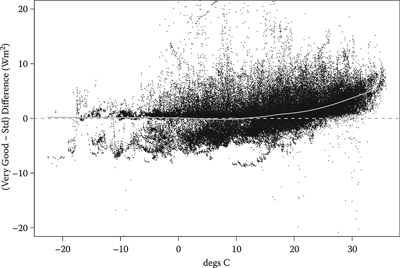
FIGURE 4.6 The temperature dependence of one very good pyrheliometer after all manufacturer’s corrections applied.
Figures 9 and 10 in Michalsky et al. (2011) illustrate the effects of correcting and not correcting the temperature dependence of pyrheliometers. Figure 4.6 is a plot of the difference in irradiance measurements between a very good thermopile pyrheliometer and a cavity radiometer after all known temperature corrections have been made. The cavity radiometer has no temperature dependence; therefore, the figure indicates that, although most of the temperature dependence is removed, there is room for improvement in the thermopile pyrheliometer at the higher ambient temperatures. Algorithms can be developed from data using ambient air temperature as a proxy for the correction. The bottom line is that every appropriate attempt to correct for this effect will reduce the uncertainty of the direct normal irradiance measurement
4.6.2 SOLAR ZENITH ANGLE DEPENDENCE
This uncertainty is not included in Table 4.5 but is of significant concern in some models of pyrheliometers This effect is not understood but is clearly illustrated, for example, in Figure 4.7, which gives data from a broadband outdoor radiometer calibration (NREL, 2010) at the Southern Great Plains Atmospheric Radiation Measurement Facility of the U.S. Department of Energy. The figure is a plot of the calibrated responsivity over a day with a responsivity change of over 2% from 80 ° to 20° solar zenith angle during the morning and almost no change from 20 ° to 80° in the afternoon Sometimes this change is smaller, and sometimes it is more symmetric about solar noon This behavior is not uncommon for some pyrheliometers, and it exceeds the uncertainty of any contribution listed in Table 4.5.

FIGURE 4.7 Solar zenith angle dependence of the Eppley NIP 29008E6 pyrheliometer during a 2010 broadband outdoor radiometer calibration (BORCAL). Note that the morning and afternoon responsivities differ as a function of solar zenith angle.
4.7 Uncertainty Analysis for Rotating Shadowband Radiometer Measurements of Direct Normal Irradiance
Rotating shadowband radiometers derive direct normal irradiance by subtracting measured diffuse horizontal from measured global horizontal irradiance and dividing by the cosine of the calculated solar zenith angle at the time of measurement. Since the uncertainty associated with the GHI is larger than the uncertainty associated with the DNI measured by a pyrheliometer, the uncertainty of the calculated DNI, which includes the uncertainties of the GHI and DHI, will necessarily be even larger. Further, there is a small uncertainty associated with the solar position calculation, which is negligible with the best algorithms, and there is an additional uncertainty associated with the horizontal leveling of the pyranometer Since most rotating shadowband radiometers use a photodiode pyranometer, there is a significant additional uncertainty associated with the nonuniform spectral response between 400 and 1100 nm and the nonresponse between 300 and 400 nm and beyond 1100 nm. Other significant uncertainty issues are the temperature dependence of the silicon cell’s response function and the angular (cosine) response of the photodiode pyranometer (see chapter 5 for more details on photodiode pyranometers). Table 4.6 lists some of the major contributors to uncertainty for a rotating shadowband radiometer that uses a photodiode pyranometer for the calculation of the direct irradiance. The expanded uncertainty for a 95% confidence in the direct irradiance calculation is 3.226%. Certain factors have very little effect on the overall uncertainty of an instrument For example, if we eliminate from Table 4.6 the uncertainties associated with the nonlinearity, the voltage resolution, and the voltage measurement standard deviation, then the combined standard uncertainty decreases by only 0.022%. Therefore, it is important to account for the large contributors to uncertainty, and many of the minor contributors to uncertainty can safely be ignored. One should first be certain that the contribution is small, however, before neglecting it.
TABLE 4.6
One Estimate of the Standard Uncertainty of a Rotating Shadowband Radiometer
|

The assumptions made for Table 4.6 were that the calibration was derived for the calculated direct normal irradiance. Had one calibrated the photodiode pyranometer for global horizontal irradiance, the uncertainty of the direct would have been greater. Most RSRs use the GHI calibration factor. For example, Michalsky, Augustine, and Kiedron (2009) demonstrated that the calibration for the global horizontal and for the direct normal irradiances are different by about 2.5% for the photodiode pyranometer as used in that paper. There would be similar differences for other photodiode pyranometers. In Table 4.6, the temperature dependence is not corrected; there is about a 3% change over typical annual operating temperatures If this temperature is measured and the correction is made, then this contribution to the uncertainty drops significantly to around 0.3%. Similarly, if the cosine response is measured and a correction applied to the direct beam calculation, this large contribution to the uncertainty can be reduced to a much smaller number, perhaps as low as 0.4%. In Table 4.6 it is assumed that there has been a correction applied to reduce the uncertainty of the spectral correction to 1.0%. However, this contribution to the uncertainty will dominate rotating shadowband radiometer measurement uncertainty if not corrected properly For more discussion of RSRs and photodiode pyranometers see Chapters 5 and 7.
4.8 Direct Normal Irradiance Models
The term model has different meanings. Two types of models are briefly discussed here. First, we discuss models that are radiative transfer codes that require inputs to these codes to describe the atmospheric extinction sources in the path of the direct solar beam. The second type of model uses satellite images or atmospheric soundings as observed from satellites to estimate the direct solar radiation that strikes the earth’s surface.
4.8.1 GROUND-BASED MODELING
Clear-sky direct irradiance radiative transfer models perform very well if model inputs are accurately specified. Michalsky et al. (2006) evaluated six direct irradiance models of varying complexity. For the 30 cases studied, it was demonstrated that the estimated clear-sky DNI values differed from measurements by less than 1%. The mean difference for the six models was 0.5%. This implies that radiative transfer models are well developed, and, given the correct input parameters, one can estimate clear-sky DNI values to an accuracy of better than field pyrheliometer measurements. So, why are models not preferred over measurements? The reason is that good models need several accurately specified input parameters to yield correct broadband irradiances. Aerosol optical depth (AOD) and some indication of its wavelength dependence are needed The wavelength dependence can be a simple Ångström expression such as T = ¡iX∼a, which will be discussed in Chapter 12. The next most important contributor to direct beam extinction is water vapor, so one requires some estimate of this quantity, and finally, an ozone column measurement or estimate is needed. Daily column ozone can be obtained from the NASA website (http://toms.gsfc.nasa.gov/teacher/ozone_overhead_v8.xhtml). Water vapor can be crudely estimated from surface relative humidity or, better yet, using nearby radiosondes, if available Aerosol optical depths are measured with sun radiometers, which are not widely available, and will be discussed in Chapter 12. If one’s goal is to measure or model direct irradiance, AOD or direct normal irradiance measurements present different but similar measurement challenges The more complex models of the spectral distribution of direct normal irradiance, which can be integrated to calculate broadband solar irradiance, are discussed in Chapter 12.
4.8.2 SATELLITE MODEL ESTIMATES
Satellite estimates of surface solar irradiance use models that range in complexity from those based on regressions of ground-based measurements to satellite pixel brightness (i e, completely empirical) to those based on radiative transfer models using satellite-retrieved or climatological information on cloud properties, aerosols, humidity, and temperature profiles
Perez et al. (2002) published their paper on a well-known operational model for deriving surface irradiance from satellite measurements that has a hybrid approach. The technique uses the pixel brightness as measured by the Geostationary Operational Environmental Satellites (GOES) but takes into account the site’s elevation, a climatological estimate of the monthly average aerosol loading, snow cover, and a specular reflectance correction factor. Clean Power Research uses this model and its modifications of it for its SolarAnywhere service, which provides estimates of surface irradiance (http://www.cleanpower.com/SolarAnywhere), including direct normal irradiance. 3TIER (http://www.3tier.com/en/products/) processes satellite data to generate surface irradiance using its own modified version of the Perez et al. model. A popular site for solar direct normal irradiance information based on satellite retrievals of the input parameters is the NASA Surface meteorology and Solar Energy (SSE) website (http://power.larc.nasa.gov). This is also known as the Prediction Of Worldwide Energy Resource (POWER) project website. NASA’s SSE approach is a more physics-based approach in that it uses a radiative transfer code with cloud optical property inputs from satellite retrievals and a chemical transport model to estimate aerosol extinction to calculate surface solar direct normal irradiance
The uncertainties associated with satellite retrievals of direct normal irradiances are about twice as large as those for the retrievals of global horizontal irradiance from satellites. Satellite estimates of hourly DNI using the Perez et al. (2002) model have biases of only a few percent and root mean square errors (RMSEs) in the 35–40% range for hourly data (e .g., Vignola, Harlan, Perez, and Kmiecik, 2007). In Vignola et al. the RMSE and the mean bias error (MBE) of DNI are calculated from hourly averages of frequently sampled ground-based (gnd) measurements and one satellite image (sat) per hour. The MBE in percent is calculated using
where the sum is ideally formed over all the daylight hours in at least one year to determine a typical MBE for a site. For the RMSE Vignola et al. (2007) use
where again the sum is ideally formed over all of the daylight hours in at least one year to determine a typical RMSE for a site.
As an aside, it may seem that a more straightforward way to calculate MBE in percent would be to use a formula such as
where the individual percent differences are averaged; however, if a single gndt value were equal to zero, MBE becomes undefined. If zeros were screened from the sum, small nonzero denominators would still produce large fractions that would have a large and detrimental influence on the result. The same arguments apply to calculating the RMSE using
The hourly RMSEs of 35–40% may seem high because MBEs and RMSEs are often quoted for mean monthly daily totals, which are much smaller numbers. For example, Myers, Wilcox, Marion, George, and Anderberg (2005) quote uncertainties around 14% for the sites in their study using Perez et al.’s (2002) model. The average monthly daily total (AMDT) is the total solar energy per square meter per day summed over all days in the month divided by the number of days in the month Every month is likely to have direct sunlight; therefore, this calculation of MBE
is likely to give a valid and defined MBE. In this equation gnd. and sat{ are AMDTs for one of the m months in the sample size. Note this has the same form as Equation 4.6, but instead of summing over individual hours the sum is over monthly averages of daily totals The same argument applies to the RMSE for AMDTs Alternately, it would be as informative to calculate and compare MBE and RMSE using equations of the form in (4.4) and (4 .5). It is useful to state just how MBE and RMSE are calculated when quoting biases and uncertainties, and it should be required for publications.
4.9 Historical and Current Surface-Measured Direct Normal Irradiance Data
An excellent review of the historical solar irradiance data and accompanying metadata regarding these can be found in Stoffel et al. (2010) and need not be repeated here. Years of calibrated and well-maintained instrumentation that captures as complete a record of direct normal irradiance data as possible are critical in understanding the annual and interannual variability of radiation. Climate research and central concentrating solar power generation require long records to understand the longterm variability of DNI
In this section, only current (as of June 2011) measurements of direct normal irradiance with expectations of continuance will be discussed. Much of the focus, but not all, is on the United States and on measurements made with first-class instruments. Rotating shadowband radiometers will be discussed because of their proliferation
The Baseline Surface Radiation Network (BSRN) was started by the World Climate Research Program in 1992 to measure solar and infrared surface radiation with the highest-quality instruments and techniques available (Ohmura et al., 1998). The data produced have been used for validating and improving satellite retrievals of surface radiative fluxes, for comparisons to climate model calculations, and for monitoring subtle long-term changes in the surface radiative environment. The database is maintained at the Alfred Wegener Institute in Bremerhaven, Germany. Data are available from about 50 stations worldwide at http://www.bsrn.awi.de.

FIGURE 4.8 Hourly average DNI for Burns, Eugene, and Hermiston, Oregon, for the years from 1978 through 2010; monthly average hourly values are used to determine the annual average. The monthly average values exclude hours or days with missing data or misaligned measurements.
The World Radiation Data Center is in St. Petersburg, Russia. It was established by the World Meteorological Organization to archive and publish solar radiation data. Most of the data from the more than 1000 sites included in the archive are GHI measurements representing daily total irradiation values Some sites submit hourly data, and some sites submit DNI*.
In the United States, three small networks continue to provide moderate-to high-quality direct normal irradiance data: the University of Oregon Solar Radiation Monitoring Laboratory (UO SRML), the NOAA Surface Radiation (SURFRAD) network, and the NOAA Integrated Surface Irradiance Study (ISIS) network.
The UO SRML has run the Pacific Northwest (United States) Solar Radiation Data Network since 1977. The annual average DNI from the three longest running stations is shown in Figure 4.8. Currently, 12 stations operate in Idaho, Montana, Oregon, Utah, Washington, and Wyoming to measure direct normal irradiance; five stations use pyrheliometers, and seven stations use RSRs. Eugene and Hermiston, Oregon, have colocated RSRs and pyrheliometers to evaluate the accuracy of the RSRs. Data are taken at 5-minute intervals at most sites, although 1-minute and 15-minute data are taken at a few stations. More information can be found at http://solardata.uoregon.edu/.
* The contact information is: Voeikov Main Geophysical Observatory World Radiation Data Centre 7, Karbyshev Str. 194021, St. Petersburg, Russian Federation Voice: (812) 297–43–90 Fax: (812) 297–86–61 Director: Dr. Anatoly Tsvetkov (812) 295–04–45 t svetkov@main. mgo. rssi. ru or wrdc@main. mgo. rssi .ru
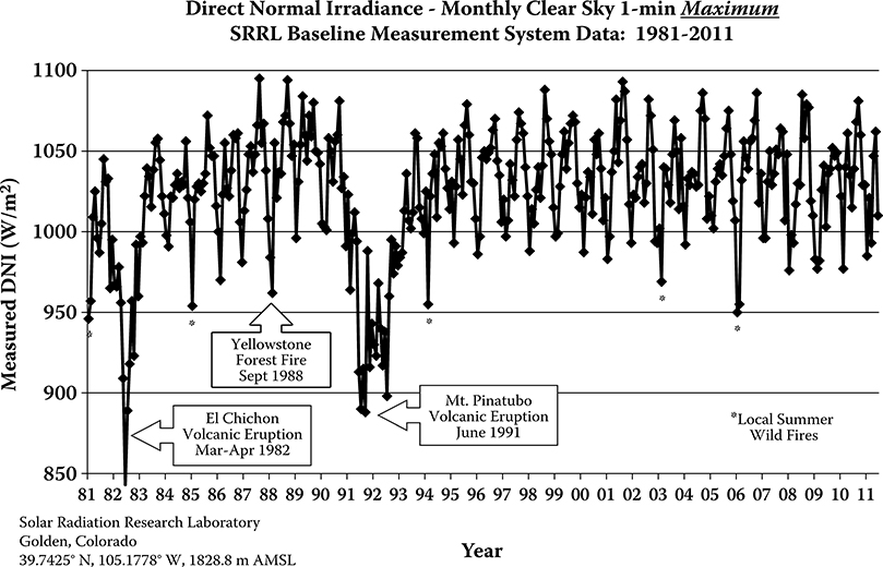
FIGURE 4.9 Maximum observed DNI for Golden, Colorado, based on 1- and 5-minute measurements from 1981 through 2011. The data have not been adjusted for sun-earth distance, showing the intra-annual and inter-annual variability. The effects of volcanic eruption and local forest fires are illustrated by the local minima.
The NOAA SURFace RADiation (SURFRAD) network has operated since 1994. All SURFRAD sites are part of the BSRN. As such the sites acquire high-quality direct solar radiation data as a subset of more extensive radiation measurements The locations of the seven sites, their data record, and much more can be found at http://www.srrb.noaa.gov/surfrad/index.xhtml.
The NOAA Integrated Surface Irradiance Study (ISIS) is a remnant of the NOAA National Weather Service solar network known as SOLRAD in the 1950s through 1980s. There are currently seven NWS stations that continue to operate solar equipment that includes direct irradiance sensors The stations and the data can be found at http://www.srrb.noaa.gov/isis/index.xhtml.
There are other medium-to high-quality direct solar irradiance measurements made in the United States, but typically their operation is short-term; the National Renewable Energy Laboratory’s (NREL) web page lists several of these (http://www.nrel.gov/midc/). NREL’s high-quality data from the Solar Radiation Research Laboratory (SRRL) in Golden, Colorado, dates from 1981 (see Figure 4.9). The U.S. Department of Energy operates the Atmospheric Radiation Measurement (ARM) site in northern Oklahoma (Stokes and Schwartz, 1994). High-quality and redundant measurements of solar direct irradiance have been made since 1992 at the ARM central facility between Lamont and Billings, Oklahoma, and at nearly 20 extended facilities through central Oklahoma and into Kansas. The extended facilities have recently been reduced to nine sites nearer the central facility.
Questions
How are global horizontal, direct normal, and diffuse horizontal irradiances related?
Name three reasons that the DNI detected at the earth’s surface is less than at the top of the atmosphere.
What is the main reason that the extraterrestrial radiation from the sun changes throughout the year? How large can this change be?
Rank these DNI measurements in order of accuracy with best first: thermo pile pyrheliometer, GOES satellite retrieval, absolute cavity radiometer.
What is the major advantage of the rotating shadowband radiometer for measuring DNI? Name two disadvantages.
How would one obtain a pyrheliometer calibration that is linked to the WRR?
What is a good reference for choosing a pyrheliometer with proven accuracy?
Did the direct normal irradiance reach 700 Wm–2 in Eugene, Oregon, on January 1, 2009? Hints: This can be checked in five clicks. How about January 2, 2009? One more click.
How many Dobson units of ozone were over Denver (40°, –105°) on March 31, 2010?
What should accompany every measurement of DNI?
References
Cook, R. R. 2002. Assessment of uncertainties of measurement for calibration and testing laboratories. National Association of Testing Authorities, Australia. Available from: http://www.nata.asn.au/publications/uncertainty
Finsterle, W. 2006. WMO International Pyrheliometer Comparison IPC-X, final report. IOM report No. 91. WMO/TD 1320, Geneva.
Gueymard, C. 1998. Turbidity determination from broadband irradiance measurements: A detailed multicoefficient approach. Journal of Applied Meteorology, 37:414–435.
ISO. 1990. Specification and classification of instruments for measuring hemispherical solar and direct solar radiation. ISO 9060, Geneva. Available from: http://www.iso.org/
Joint Committee for Guides in Metrology (JCGM). 2008. Evaluation of measurement data— Guide to the expression of uncertainty in measurement. GUM 1995 with minor revisions, Bureau International des Poids et Mesures. Available from: http://www.bipm.org/en/publications/guides/gum.xhtml
Kopp, G. and J. L. Lean, 2011. A new, lower value of total solar irradiance: Evidence and climate significance. Geophysical Research Letters, 38: L01706. doi: 10.1029/2010GL045777. LI-COR,Inc. 1982. LI–2020 automatic solar tracker instruction manual. Publication No. 8203–8227. Lincoln, NE.
Michalsky, J. J., G. P. Anderson, J. Barnard, J. Delamere, C. Gueymard, S. Kato, P. Kiedron, A. McComiskey, and P. Ricchiazzi. 2006. Shortwave radiative closure studies for clear skies during the atmospheric radiation measurement 2003 aerosol intensive observation period. Journal of Geophysical Research, 111: D14S90. doi: 10.1029/2005JD006341.
Michalsky, J. J., J. A. Augustine, and P. W. Kiedron. 2009. Improved broadband solar irradiance from the multi-filter rotating shadowband radiometer. Solar Energy 83:2144–2156.
Michalsky, J., E. G. Dutton, D. Nelson, J. Wendell, S. Wilcox, A. Andreas, P. Gotseff, D. Myers, I. Reda, T. Stoffel, K. Behrens, T. Carlund, W. Finsterle, and D. Halliwell. 2011. An extensive comparison of commercial pyrheliometers under a wide range of routine observing conditions. Journal of Atmospheric and Oceanic Technology, 28:752–766.
Myers, D. R., S. Wilcox, W. Marion, R. George, and M. Anderberg. 2005. Broadband model performance for an updated national solar radiation database in the United States of America. Proceedings of the ISES Solar World Conference, Orlando, FL.
NREL. 2010. Broadband outdoor radiometer calibration (BORCAL 2010–02). August 5, National Renewable Energy Laboratory.
Ohmura, A., H. Gilgen, H. Hegner, G. Müller, M. Wild, E. G. Dutton, B. Forgan, C. Fröhlich, R. Philipona, A. Heimo, G. König-Langlo, B. McArthur, R. Pinker, C. H. Whitlock, and K. Dehne. 1998. Baseline Surface Radiation Network (BSRN/WCRP): New precision radi-ometry for climate research. Bulletin of the American Meteorological Society 79:2115–2136.
Perez, R., P. Ineichen, K. Moore, M. Kmiecik, C. Chain, R. George, and F. Vignola. 2002. A new operational satellite-to-irradiance model. Solar Energy 73:307–317.
Reda, I. 1996. Calibration of a solar absolute cavity radiometer with traceability to the World Radiometric Reference. National Renewable Energy Laboratory NREL/TP–463–20619, Golden, CO
Reda, I., D. Myers, and T. Stoffel. 2008. Uncertainty estimate for the outdoors calibration of solar pyranometers: A metrologist perspective. Journal of Measurement Science, 3:58–66.
Stoffel, T. and I. Reda. 2009. NREL Pyrheliometer Comparisons, September 22-October 3. (NPC–2008). NREL/TP–550–45016, February, National Renewable Energy Laboratory, Golden, CO http://www.nrelgov/publications
Stoffel, T., D. Renne, D. Myers, S. Wilcox, M. Sengupta, R. George, and C. Turchi. 2010. Concentrating solar power; best practices handbook for the collection and use of solar resource data. Technical Report NREL/TP–550–47465. National Renewable Energy Laboratory, Golden, CO. http://www.nrel.gov/docs/fy10osti/47465.pdf
Stokes, G. M. and S. E. Schwartz. 1994. The Atmospheric Radiation Measurement (ARM) program: Programmatic background and design of the cloud and radiation test bed. Bulletin of The American Meteorological Society, 75:1201–1221. doi: 10.1175/1520–0477.
Taylor, B. N. and C. E. Kuyatt. 1994. Guidelines for evaluation and expressing the uncertainty of NIST measurement results. NIST Technical Note 1297, National Institute of Standards and Technology, Gaithersburg, MD. Available from: http://physics.nist.gov/cuu/Uncertainty/basic.xhtml
Vignola, F., P. Harlan, R. Perez, and M. Kmiecik. 2005. Analysis of satellite derived beam and global solar radiation data. Proceedings of the ISES Solar World Conference, Orlando, FL.
Vignola, F., P. Harlan, R. Perez, and M. Kmiecik. 2007. Analysis of satellite derived beam and global solar radiation data. Solar Energy 81:768–772.
Wesely, M. L. 1982. Simplified techniques to study components of solar radiation under haze and clouds. Journal of Applied Meteorology 21:373–383.
WMO 2008 WMO guide to meteorological instruments and methods of observation WMO-No. 8 (7th ed. ), Chapter 7. Available from: http://www.wmo.int/pages/prog/www/IMOP/publications/CIMO-Guide/CIMO_Guide–7th_Edition–2008.xhtml