
Fourier Analysis for Continuous-Time Signals and Systems
Chapter Objectives
- Learn techniques for representing continuous-time periodic signals using orthogonal sets of periodic basis functions.
- Study properties of exponential, trigonometric and compact Fourier series, and conditions for their existence.
- Learn the Fourier transform for non-periodic signals as an extension of Fourier series for periodic signals.
- Study properties of the Fourier transform. Understand energy and power spectral density concepts.
- Explore frequency-domain characteristics of CTLTI systems. Understand the system function concept.
- Learn the use of frequency-domain analysis methods for solving signal-system interaction problems with periodic and non-periodic input signals.
4.1 Introduction
In Chapters 1 and 2 we have developed techniques for analyzing continuous-time signals and systems from a time-domain perspective. A continuous-time signal can be modeled as a function of time. A CTLTI system can be represented by means of a constant-coefficient linear differential equation, or alternatively by means of an impulse response. The output signal of a CTLTI system can be determined by solving the corresponding differential equation or by using the convolution operation.
In Chapter 1 we have also discussed the idea of viewing a signal as a combination of simple signals acting as “building blocks”. Examples of this were the use of unit-step, unit-ramp, unit-pulse and unit-triangle functions for constructing signals (see Section 1.3.2) and the use of the unit-impulse function for impulse decomposition of a signal (see Section 1.3.3).
Another especially useful set of building blocks is a set in which each member function has a unique frequency. Representing a signal as a linear combination of single-frequency building blocks allows us to develop a frequency-domain view of a signal that is particularly useful in understanding signal behavior and signal-system interaction problems. If a signal can be expressed as a superposition of single-frequency components, knowing how a linear and time-invariant system responds to each individual component helps us understand overall system behavior in response to the signal. This is the essence of frequency-domain analysis.
In Section 4.2 we discuss methods of analyzing periodic continuous-time signals in terms of their frequency content. Frequency-domain analysis methods for non-periodic signals are presented in Section 4.3. In Section 4.4 representation of signal energy and power in the frequency domain is discussed. System function concept is introduced in Section 4.5. The application of frequency-domain analysis methods to the analysis of CTLTI systems is discussed in Sections 4.6 and 4.7.
4.2 Analysis of Periodic Continuous-Time Signals
Most periodic continuous-time signals encountered in engineering problems can be expressed as linear combinations of sinusoidal basis functions, the more technical name for the so-called “building blocks” we referred to in the introductory section. The idea of representing periodic functions of time in terms of trigonometric basis functions was first realized by French mathematician and physicist Jean Baptiste Joseph Fourier (1768-1830) as he worked on problems related to heat transfer and propagation. The basis functions in question can either be individual sine and cosine functions, or they can be in the form of complex exponential functions that combine sine and cosine functions together.
Later in this section we will study methods of expressing periodic continuous-time signals in three different but equivalent formats, namely the trigonometric Fourier series (TFS), the exponential Fourier series (EFS) and the compact Fourier series (CFS). Before we start a detailed study of the mathematical theory of Fourier series, however, we will find it useful to consider the problem of approximating a periodic signal using a few trigonometric functions. This will help us build some intuitive understanding of frequency-domain methods for analyzing periodic signals.
4.2.1 Approximating a periodic signal with trigonometric functions
It was established in Section 1.3.4 of Chapter 1 that a signal ˜x(t) which is periodic with period T0 has the property
˜x(t+T0)=˜x(t)(4.1)
for all t. Furthermore, it was shown through repeated use of Eqn. (4.1) that a signal that is periodic with period T0 is also periodic with kT0 for any integer k.
In working with periodic signals in this chapter, we will adopt the convention of using the tilde (~) character over the name of the signal as a reminder of its periodicity. For the sake of discussion let us consider the square-wave signal ˜x(t) with a period of T0 as shown in Fig. 4.1.

Suppose that we wish to approximate this signal using just one trigonometric function. The first two questions that need to be answered are:
- Should we use a sine or a cosine?
- How should we adjust the parameters of the trigonometric function?
The first question is the easier one to answer. The square-wave signal ˜x(t) (t) shown in Fig. 4.1 has odd symmetry signified by ˜x(-t)=-˜x(t) (see Section 1.3.6 of Chapter 1). Among the two choices for a trigonometric function, the sine function also has odd symmetry, that is, sin (− a)= −sin (a) for any real-valued parameter a. On the other hand, the cosine function has even symmetry since cos (−a) = cos(a). Therefore it would intuitively make sense to choose the sine function over the cosine function. Our approximation would be in the form
˜x(t)≈b1sin(ωt)(4.2)
Since ˜x(t) has a fundamental period of T0, it would make sense to pick a sine function with the same fundamental period, so that
sin(ω(t+T0))=sin(ωt)(4.3)
For Eqn. (4.3) to work we need ωT0 = 2π and consequently
ω=2πT0=ω0=2πf0(4.4)
where we have defined the frequency f0 as the reciprocal of the period, that is, f0 = 1/T0. Let ˜x(1)(t) represent an approximate version of the signal ˜x(t), so that
˜x(1)(t)=b1sin(ω0t)(4.5)
In Eqn. (4.5) we have used the superscripted signal name ˜x(1) to signify the fact that we are using only one trigonometric function in this approximation. Our next task is to determine the value of the coefficient b1. How should b1 be chosen that Eqn. (4.5) represents the best approximation of the given type possible for the actual signal ˜x(t)? There is a bit of subjectivity in this question since we have not yet defined what the “best approximation” means for our purposes.
Let us define the approximation error as the difference between the square-wave signal and its approximation:
˜ɛ1(t)=˜x(t)-˜x(t)-b1sin(ω0t)(4.6)
The subscript used on the error signal ˜ɛ1(t) signifies the fact that it is the approximation error that results when only one trigonometric function is used. ˜ɛ1(t) is also periodic with period T0. One possible method of choosing the best value for the coefficient b1 would be to choose the value that makes the normalized average power of ˜ɛ1(t) as small as possible.
Recall that the normalized average power in a periodic signal was defined in Chapter 1 Eqn. (1.88). Adapting it to the error signal ˜ɛ1(t) we have
P∈=1T0∫T00[˜ɛ1(t)]2dt(4.7)
This is also referred to as the mean-squared error (MSE). For simplicity we will drop the constant scale factor 1/T0 in front of the integral in Eqn. (4.7), and minimize the cost function
J=∫T00[˜ɛ1(t)]2dt=∫T00[˜x(t)-b1sin(ω0t)]2dt(4.8)
instead. Minimizing J is equivalent to minimizing P∈ since the two are related by a constant scale factor. The value of the coefficient b1 that is optimum in the sense of producing the smallest possible value for MSE is found by differentiating the cost function with respect to b1 and setting the result equal to zero.
dJdb1=ddb1[∫T00[˜x(t)-b1sin(ω0t)]2dt]=0
Changing the order of integration and differentiation leads to
dJdb1=∫T00ddb1[˜x(t)-b1sin(ω0t)]2dt=0
Carrying out the differentiation we obtain
∫T002[˜x(t)-b1sin(ω0t)][-sin(ω0t)]dt=0
or equivalently
∫T00˜x(t)sin(ω0t) dt+b1∫T00sin2(ω0t)dt=0(4.9)
It can be shown that the second integral in Eqn. (4.9) yields
∫T00sin2(ω0t) dt=T02
Substituting this result into Eqn. (4.9) yields the optimum choice for the coefficient b1 as
b1=2T0∫T00˜x(t)sin(ω0t) dt(4.10)
For the square-wave signal ˜x(t) in Fig. 4.1 we have
b1=2T0∫T0/20(A)sin(ω0t) dt+2T0∫T0T0/2(-A) sin(ω0t) dt=4Aπ(4.11)
The best approximation to ˜x(t) using only one trigonometric function is
˜x(1)(t)=4Aπ sin(ω0t)(4.12)
and the approximation error is
˜ɛ1(t)=˜x(t)-4Aπsin(ω0t)
The signal ˜x(t), its single-frequency approximation ˜x(1)(t) and the approximation error ˜ɛ1(t) are shown in Fig. 4.2.

(a) The square-wave signal ˜x(t) and its single-frequency approximation ˜x(1)(t), (b) the approximation error ˜ɛ1(t).
In the next step we will try a two-frequency approximation to ˜x(t) and see if the approximation error can be reduced. We know that the basis function sin (2ω0t) = sin (4πf0t) is also periodic with the same period T0; it just has two full cycles in the interval (0, T0) as shown in Fig. 4.3.

Let the approximation using two frequencies be defined as
˜x(2)(t)=b1sin(ω0t)+b2sin(2ω0t)(4.14)
The corresponding approximation error is
˜ɛ2(t)=˜x(t)-˜x(2)(t)=˜x(t)-b1sin(ω0t)-b2sin(2ω0t)(4.15)
The cost function will be set up in a similar manner:
J=∫T00[˜x(t)-b1sin(ω0t)-b2sin(2ω0t)]2dt(4.16)
Differentiating J with respect to first b1 and then b2 we obtain
∂J∂b1=∫T002[˜x(t)-b1sin(ω0t)-b2sin(2ω0t)][-sin(ω0t)] dt
and
Setting the partial derivatives equal to zero leads to the following two equations:
We have already established that
Similarly it can be shown that
and Eqns. (4.17) and (4.18) can now be solved for the optimum values of the coefficients b1 and b2, resulting in
and
It is interesting to note that the expression for b1 given in Eqn. (4.19) for the two-frequency approximation problem is the same as that found in Eqn. (4.10) for the single-frequency approximation problem. This is a result of the orthogonality of the two sine functions sin (ω0t) and sin (2ω0t), and will be discussed in more detail in the next section.
Using the square-wave signal in Eqns. (4.19) and (4.20) we arrive at the following optimum values for the two coefficients:
Interestingly, the optimum contribution from the sinusoidal term at radian frequency 2ω0 turned out to be zero, resulting in
for this particular signal .
It can be shown (see Problem 4.1 at the end of this chapter) that a three-frequency approximation
has the optimum coefficient values
The signal , its three-frequency approximation and the approximation error are shown in Fig. 4.4.

(a) The square-wave signal and its three-frequency approximation , (b) the approximation error .
Some observations are in order:
- Based on a casual comparison of Figs. 4.2(b) and 4.4(b), the normalized average power of the error signal seems to be less than that of the error signal . Consequently, is a better approximation to the signal than .
- On the other hand, the peak value of the approximation error seems to be ±A for both and . If we were to try higher-order approximations using more trigonometric basis functions, the peak approximation error would still be ±A (see Problem 4.4 at the end of this chapter). This is due to fact that, at each discontinuity of , the value of the approximation is equal to zero independent of the number of trigonometric basis functions used. In general, the approximation at a discontinuity will yield the average of the signal amplitudes right before and right after the discontinuity. This leads to the well-known Gibbs phenomenon, and will be explored further in Section 4.2.6.
Interactive Demo: appr demo1
The demo program in "appr demo1.m" provides a graphical user interface for experimenting with approximations to the square-wave signal of Fig. 4.1 using a specified number of trigonometric functions. Parameter values A = 1 and T0 = 1 s are used. On the left side, slider controls allow parameters bi to be adjusted freely for i = 1, ..., 7. The approximation
and the corresponding approximation error
are computed and graphed. The value of m may be controlled by setting unneeded coefficients equal to zero. For example , the approximation with 5 trigonometric terms, may be explored by simply setting b6 = b7 = 0 and adjusting the remaining coefficients. In addition to graphing the signals, the program also computes the value of the cost function
- With all other coefficients reset to zero, adjust the value of b1 until J becomes as small as possible. How does the best value of b1 correspond to the result found in Eqn. (4.12)? Make a note of the smallest value of J obtained.
- Keeping b1 at the best value obtained, start adjusting b2. Can J be further reduced through the use of b2?
- Continue in this manner adjusting the remaining coefficients one at a time. Observe the shape of the approximation error signal and the value of J after each adjustment.
Software resources:
appr demo1.m
4.2.2 Trigonometric Fourier series (TFS)
We are now ready to generalize the results obtained in the foregoing discussion about approximating a signal using trigonometric functions. Consider a signal that is periodic with fundamental period T0 and associated fundamental frequency f0 = 1/T0. We may want to represent this signal using a linear combination of sinusoidal functions in the form
or, using more compact notation
where ω0 = 2πf0 is the fundamental frequency in rad/s. Eqn. (4.26) is referred to as the trigonometric Fourier series (TFS) representation of the periodic signal , and the sinusoidal functions with radian frequencies of ω0, 2ω0, ..., kω0 are referred to as the basis functions. Thus, the set of basis functions includes
and
Using the notation established in Eqns. (4.27) and (4.28), the series representation of the signal given by Eqn. (4.25) can be written in a more generalized fashion as
We will call the frequencies that are integer multiples of the fundamental frequency the harmonics. The frequencies 2ω0, 3ω0, ..., kf0 are the second, the third, and the k-th harmonics of the fundamental frequency respectively. The basis functions at harmonic frequencies are all periodic with a period of T0. Therefore, considering our “building blocks” analogy, the signal which is periodic with period T0 is represented in terms of building blocks (basis functions) that are also periodic with the same period. Intuitively this makes sense.
Before we tackle the problem of determining the coefficients of the Fourier series representation, it is helpful to observe some properties of harmonically related sinusoids. Using trigonometric identities it can be shown that
This is a very significant result. Two cosine basis functions at harmonic frequencies ω0 and kω0 are multiplied, and their product is integrated over one full period (t0, t0 + T0). When the integer multipliers m and k represent two different harmonics of the fundamental frequency, the result of the integral is zero. A non-zero result is obtained only when m = k, that is, when the two cosine functions in the integral are the same. A set of basis functions {cos (kω0t), k = 0, ..., ∞} that satisfies Eqn. (4.30) is said to be an orthogonal set. Similarly it is easy to show that
meaning that the set of basis functions {sin (kω0t), k = 1, ..., ∞} is orthogonal as well. Furthermore it can be shown that the two sets are also orthogonal to each other, that is,
for any combination of the two integers m and k (even when m = k). In Eqns. (4.30) through (4.32) the integral on the left side of the equal sign can be started at any arbitrary time instant t0 without affecting the result. The only requirement is that integration be carried out over one full period of the signal.
Detailed proofs of orthogonality conditions under a variety of circumstances are given in Appendix D.
We are now ready to determine the unknown coefficients {ak; k = 0, 1, ..., ∞} and {bk; k = 1, ..., ∞} of Eqns. (4.25) and (4.26). Let us first change summation indices in Eqn. (4.26) from k to m, then multiply both sides of it with cos (kω0t) and integrate over one full period:
Swapping the order of integration and summation in Eqn. (4.33) leads to
Let us consider the three terms on the right side of Eqn. (4.34) individually:
- Let k > 0 (we will handle the case of k = 0 separately). The first term on the right side of Eqn. (4.34) evaluates to zero since it includes, as a factor, the integral of a cosine function over a full period.
- In the second term we have a summation. Each term within the summation has a factor which is the integral of the product of two cosines over a span of T0. Using the orthogonality property observed in Eqn. (4.30), it is easy to see that all terms in the summation disappear with the exception of one term for which m = k.
- In the third term we have another summation. In this case, each term within the summation has a factor which is the integral of the product of a sine function and a cosine function over a span of T0. Using Eqn. (4.32) we conclude that all terms of this summation disappear.
Therefore, Eqn. (4.34) simplifies to
which can be solved for the only remaining coefficient ak to yield
Similarly, by multiplying both sides of Eqn. (4.26) with sin (kω0t) and repeating the procedure used above, it can be shown that bk coefficients can be computed as (see Problem 4.6 at the end of this chapter)
Finally, we need to compute the value of the constant coefficient a0. Integrating both sides of Eqn. (4.26) over a full period, we obtain
Again changing the order of integration and summation operators, Eqn. (4.36) becomes
Every single term within each of the two summations will be equal to zero due to the periodicity of the sinusoidal functions being integrated. This allows us to simplify Eqn. (4.38) to
which can be solved for a0 to yield
A close examination of Eqn. (4.39) reveals that the coefficient a0 represents the time average of the signal as defined in Eqn. (1.83) of Chapter 1. Because of this, a0 is also referred to as the average value or the dc component of the signal.
Combining the results obtained up to this point, the TFS expansion of a signal can be summarized as follows:
Trigonometric Fourier series (TFS):
Synthesis equation:
Analysis equations:
Example 4.1: Trigonometric Fourier series of a periodic pulse train
A pulse-train signal with a period of T0 = 3 seconds is shown in Fig. 4.5. Determine the coefficients of the TFS representation of this signal.

Solution: In using the integrals given by Eqns. (4.41), (4.42), and (4.43), we can start at any arbitrary time instant t0 and integrate over a span of 3 seconds. Applying Eqn. (4.43) with t0 = 0 and T0 = 3 seconds, we have
The fundamental frequency is f0 = 1/T0 = 1/3 Hz, and the corresponding value of ω0 is
Using Eqn. (4.41), we have
Finally, using Eqn. (4.42), we get
Using these coefficients in the synthesis equation given by Eqn. (4.40), the signal x(t) can now be expressed in terms of the basis functions as
Example 4.2: Approximation with a finite number of harmonics
Consider again the signal of Example 4.1. Based on Eqns. (4.25) and (4.26), it would theoretically take an infinite number of cosine and sine terms to obtain an accurate representation of it. On the other hand, values of coefficients ak and bk are inversely proportional to k, indicating that the contributions from the higher order terms in Eqn. (4.44) will decline in significance. As a result we may be able to neglect high order terms and still obtain a reasonable approximation to the pulse train. Approximate the periodic pulse train of Example 4.1 using (a) the first 4 harmonics, and (b) the first 10 harmonics.
Solution: Recall that we obtained the following in Example 4.1:
These coefficients have been numerically evaluated for up to k = 10, and are shown in Table 4.1.
TFS coefficients for the pulse train of Example 4.2.
k |
ak |
bk |
|---|---|---|
0 |
0.3333 |
|
1 |
0.2757 |
0.4775 |
2 |
−0.1378 |
0.2387 |
3 |
0.0 |
0.0 |
4 |
0.0689 |
0.1194 |
5 |
−0.0551 |
0.0955 |
6 |
0.0 |
0.0 |
7 |
0.0394 |
0.0682 |
8 |
−0.0345 |
0.0597 |
9 |
0.0 |
0.0 |
10 |
0.0276 |
0.0477 |
Let be an approximation to the signal utilizing the first m harmonics of the fundamental frequency:
Using m = 4, we have
A similar but lengthier expression can be written for the case m = 10 which we will skip to save space. Fig. 4.6 shows two approximations to the original pulse train using the first 4 and 10 harmonics respectively.

The demo program in "tfs demo1.m" provides a graphical user interface for computing finite-harmonic approximations to the pulse train of Examples 4.1 and 4.2. Values of the TFS coefficients ak and bk for the pulse train are displayed in the spreadsheet-style table on the left.
Selecting an integer value m from the drop-down list labeled "Largest harmonic to include in approximation" causes the finite-harmonic approximation to be computed and graphed. At the same time, checkboxes next to the coefficient pairs {ak, bk} that are included in the approximation are automatically checked.
Alternatively coefficient sets {ak, bk} may be included or excluded arbitrarily by checking the box to each set of coefficients on or off. When this is done, the graph displays the phrase “free format” as well as a list of the coefficient indices included.
- Use the drop-down list to compute and graph various finite-harmonics approximations. Observe the similarity of the approximated signal to the original pulse train as larger values of m are used.
- Use the free format approach for observing the individual contributions of individual {ak bk} pairs. (This requires checking one box in the table with all others unchecked.)
Software resources:
tfs_demo1.m
Software resources: |
See MATLAB Exercises 4.1 and 4.2. |
Example 4.3: Periodic pulse train revisited
Determine the TFS coefficients for the periodic pulse train shown in Fig. 4.7.

Solution: This is essentially the same pulse train we have used in Example 4.1 with one minor difference: The signal is shifted in the time domain so that the main pulse is centered around the time origin t = 0. As a consequence, the resulting signal is an even function of time, that is, it has the property for −∞ < t < ∞.
Let us take one period of the signal to extend from t0 = −1.5 to t0 + T0 = 1.5 seconds. Applying Eqn. (4.43) with t0 = −1.5 and T0 = 3 seconds, we have
Using Eqn. (4.41) yields
and using Eqn. (4.42)
Thus, can be written as
where the fundamental frequency is f0 = 1/3 Hz. In this case, the signal is expressed using only the cos (kω0t) terms of the TFS expansion. This result is intuitively satisfying since we have already recognized that exhibits even symmetry, and therefore it can be represented using only the even basis functions {cos (kω0t), k = 0, 1, ..., ∞}, omitting the odd basis functions {sin (kω0t), k = 1, 2,..., ∞}.
ex_4_3.m
Interactive Demo: tfs_demo2
The demo program in “tfs demo2.m” is based on Example 4.3, and computes finite-harmonic approximations to the periodic pulse train with even symmetry as shown in Fig. 4.7. It shares the same graphical user interface as in the program “tfs demo1.m” with the only difference being the even symmetry of the pulse train used. Values of TFS coefficients ak and bk are displayed in the spreadsheet-style table on the left. Observe that bk = 0 for all k as we have determined in Example 4.3.
Software resources:
imp_demo.m
Example 4.4: Trigonometric Fourier series for a square wave
Determine the TFS coefficients for the periodic square wave shown in Fig 4.8.

Solution: This is a signal with odd symmetry, that is, for −∞ < t < ∞. Intuitively we can predict that the constant term a0 and the coefficients ak of the even basis functions {cos (kω0t), k = 1,..., ∞} in the TFS representation of should all be equal to zero, and only the odd terms of the series should have significance. Applying Eqn. (4.41) with integration limits t0 = −T0/2 and t0 + T0 = T0/2 seconds, we have
as we have anticipated. Next, we will use Eqn. (4.43) to determine a0:
Finally, using Eqn. (4.42), we get the coefficients of the sine terms:
Using the identity
the result found for bk can be written a
Compare the result in Eqn. (4.47) to the coefficients b1 through b3 we have computed in Eqn. (4.24) in the process of finding the optimum approximation to the square-wave signal using three sine terms. Table 4.2 lists the TFS coefficients up to the 10-th harmonic.
TFS coefficients for the square-wave signal of Example 4.4.
k |
ak |
bk |
|---|---|---|
0 |
0.0 |
|
1 |
0.0 |
1.2732 |
2 |
0.0 |
0.0 |
3 |
0.0 |
0.4244 |
4 |
0.0 |
0.0 |
5 |
0.0 |
0.2546 |
6 |
0.0 |
0.0 |
7 |
0.0 |
0.1819 |
8 |
0.0 |
0.0 |
9 |
0.0 |
0.1415 |
10 |
0.0 |
0.0 |
Finite-harmonic approximations of the signal for m = 3 and m = 9 are shown in Fig. 4.9(a) and (b).

Software resources:
ex_4_4a.m
ex_4_4b.m
Interactive Demo: tfs_demo3
The demo program in "tfs demo3.m" is based on the TFS representation of a square-wave signal as discussed in Example 4.4. It computes finite-harmonic approximations to the square-wave signal with odd symmetry as shown in Fig. 4.9. It extends the user interface of the programs "tfs demo1.m" and "tfs demo2.m" by allowing the amplitude A and the period T0 to be varied through the use of slider controls. Observe the following:
- When the amplitude A is varied, the coefficients bk change proportionally, as we have determined in Eqn. (4.47).
- Varying the period T0 causes the fundamental frequency f0 to also change. The coefficients bk are not affected by a change in the period. The finite-harmonic approximation to the signal changes as a result of using a new fundamental frequency with the same coefficients.
Software resources:
tfs_demo3.m
4.2.3 Exponential Fourier series (EFS)
Fourier series representation of the periodic signal in Eqn. (4.26) can also be written in alternative forms. Consider the use of complex exponentials as basis functions so that the signal is expressed as a linear combination of them in the form
where the coefficients ck are allowed to be complex-valued even though the signal is real. This is referred to as the exponential Fourier series (EFS) representation of the periodic signal. Before we consider this idea for an arbitrary periodic signal we will study a special case.
Single-tone signals:
Let us first consider the simplest of periodic signals: a single-tone signal in the form of a cosine or a sine waveform. We know that Euler’s formula can be used for expressing such a signal in terms of two complex exponential functions:
Comparing Eqn. (4.49) with Eqn. (4.48) we conclude that the cosine waveform can be written in the EFS form of Eqn. (4.48) with coefficients
If the signal under consideration is sin (ω0t + θ), a similar representation can be obtained using Euler’s formula:
Using the substitutions
Eqn. (4.51) can be written as
Comparison of Eqn. (4.52) with Eqn. (4.48) leads us to the conclusion that the sine waveform in Eqn. (4.52) can be written in the EFS form of Eqn. (4.48) with coefficients
The EFS representations of the two signals are shown graphically, in the form of a line spectrum, in Fig. 4.10(a) and (b).

The magnitudes of the coefficients are identical for the two signals, and the phases differ by π/2. This is consistent with the relationship
The general case:
We are now ready to consider the EFS representation of an arbitrary periodic signal . In order for the series representation given by Eqn. (4.48) to be equivalent to that of Eqn. (4.26) we need
and
for each value of the integer index k. Using Euler’s formula in Eqn. (4.56) yields
Since Eqn. (4.57) must be satisfied for all t, we require that coefficients of sine and cosine terms on both sides be identical. Therefore
and
Solving Eqns. (4.58) and (4.59) for ck and c−k we obtain
and
for k = 1, ..., ∞. Thus, EFS coefficients can be computed from the knowledge of TFS coefficients through the use of Eqns. (4.60) and (4.61).
Comparison of Eqns. (4.60) and (4.61) reveals another interesting result: For a real-valued signal , positive and negative indexed coefficients are complex conjugates of each other, that is,
What if we would like to compute the EFS coefficients of a signal without first having to obtain the TFS coefficients? It can be shown (see Appendix D) that the exponential basis functions also form an orthogonal set:
EFS coefficients can be determined by making use of the orthogonality of the basis function set.
Let us first change the summation index in Eqn. (4.48) from k to m. Afterwards we will multiply both sides with e−jkω0t to get
Integrating both sides of Eqn. (4.64) over one period of and making use of the orthogonality property in Eqn. (4.63), we obtain
which we can solve for the coefficient ck as
In general, the coefficients of the EFS representation of a periodic signal are complex-valued. They can be graphed in the form of a line spectrum if each coefficient is expressed in polar complex form with its magnitude and phase:
Magnitude and phase values in Eqn. (4.67) are computed by
and
respectively. Example 4.5 will illustrate this. If we evaluate Eqn. (4.66) for k = 0 we obtain
The right side of Eqn. (4.70) is essentially the definition of the time average operator given by Eqn. (1.83) in Chapter 1. Therefore, c0 is the dc value of the signal .
Example 4.5: Exponential Fourier series for periodic pulse train
Determine the EFS coefficients of the signal of Example 4.3, shown in Fig. 4.7, through direct application of Eqn. (4.72).
Solution: Using Eqn. (4.72) with t0 = −1.5 s and T0 = 3 s, we obtain
For this particular signal , the EFS coefficients ck are real-valued. This will not always be the case. The real-valued result for coefficients {ck} obtained in this example is due to the even symmetry property of the signal . (Remember that, in working with the same signal in Example 4.3, we found bk = 0 for all k. As a result, we have ck = c−k = ak/2 for all k.)
Before the coefficients {ck} can be graphed or used for reconstructing the signal the center coefficient c0 needs special attention. Both the numerator and the denominator of the expression we derived in Eqn. (4.73) become zero for k = 0. For this case we need to use L’Hospital’s rule which yields
The signal can be expressed in terms of complex exponential basis functions as
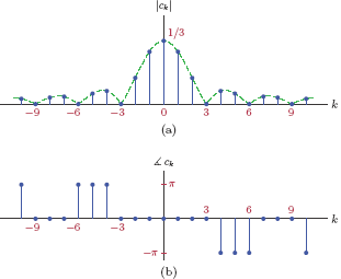
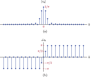
A line graph of the set of coefficients ck is useful for illustrating the make-up of the signal in terms of its harmonics, and is shown in Fig. 4.11.
Note that this is not quite in the magnitude-and-phase form of the line spectrum discussed earlier. Even though the coefficients {ck} are real-valued, some of the coefficients are negative. Consequently, the graph in Fig. 4.11 does not qualify to be the magnitude of the spectrum. Realizing that ejπ = −1, any negative-valued coefficient ck < 0 can be expressed as

using a phase angle of π radians to account for the negative multiplier. The line spectrum is shown in Fig. 4.12 in its proper form.
Interactive Demo: efs_demo1
The demo program in "efs demo1.m" is based on Example 4.5, and provides a graphical user interface for computing finite-harmonic approximations to the pulse train of Fig. 4.7. Values of the EFS coefficients ck are displayed in Cartesian format in the spreadsheet-style table on the left.
Selecting an integer value m from the drop-down list labeled “Largest harmonic to include in approximation” causes the finite-harmonic approximation to be computed and graphed. At the same time, checkboxes next to the coefficients ck included in the finite-harmonic approximation are automatically checked.
Alternatively, arbitrary coefficients may be included or excluded by checking or unchecking the box next to each coefficient. When this is done, the graph displays the phrase “free format” as well as a list of indices of the coefficients included in computation.
- Use the drop-down list to compute and graph various finite-harmonics approximations. Observe the similarity of the approximated signal to the original pulse train as larger values of m are used.
- Use the free format approach for observing the individual contributions of individual ck coefficients by checking only one box in the table with all others unchecked.
Software resources:
efs_demo1.m
Software resources: |
See MATLAB Exercise 4.3. |
Example 4.6: Periodic pulse train revisited
In Example 4.5 the EFS coefficients of the pulse train in Fig. 4.7 were found to be purely real. As discussed, this is due to the even symmetry of the signal. In this example we will remove this symmetry to see how it impacts the EFS coefficients. Consider the pulse train shown in Fig. 4.13.

Using Eqn. (4.66) with t0 = 0 and T0 = 3 seconds we obtain
After some simplification, it can be shown that real and imaginary parts of the coefficients can be expressed as
Contrast these results with the TFS coefficients determined in Example 4.1 for the same signal. TFS representation of the signal was given in Eqn. (4.44). Recall that the EFS coefficients are related to TFS coefficients by Eqns. (4.60) and (4.61). Using Eqns. (4.68) and (4.69), magnitude and phase of ck can be computed as
and
The expression for magnitude can be further simplified. Using the appropriate trigonometric identity 1 we can write
Substituting this result into Eqn. (4.74) yields
where we have used the sinc function defined as
The line spectrum is graphed in Fig. (4.14).
Software resources:
ex_4_6.m
Interactive Demo: efs_demo2
The demo program in "efs demo2.m" is based on Example 4.6 in which we have removed the even symmetry of the pulse train of Example 4.5. If the periodic waveforms used in Examples 4.5 and 4.6 are denoted as and respectively, the relationship between them may be written as
The demo provides a graphical user interface for adjusting the time delay and observing its effects on the exponential Fourier coefficients as well as the corresponding finite-harmonic approximation.
- Observe that the magnitude spectrum ck does not change with changing time-delay.
- A delay of td = 0.5 s creates the signal in Example 4.6. Observe the phase of the line spectrum.
- On the other hand, a delay of td = 0 creates the signal in Example 4.5 with even symmetry. In this case the phase should be either 0 or 180 degrees.
efs_demo2.m
Software resources: |
See MATLAB Exercise 4.4. |
Example 4.7: Effects of duty cycle on the spectrum
Consider the pulse train depicted in Fig. 4.15.

Each pulse occupies a time duration of τ within a period length of T0. The duty cycle of a pulse train is defined as the ratio of the pulse-width to the period, that is,
The duty cycle plays an important role in pulse-train type waveforms used in electronics and communication systems. Having a small duty cycle means increased blank space between individual pulses, and this can be beneficial in certain circumstances. For example, we may want to take advantage of the large gap between pulses, and utilize the target system to process other signals using a strategy known as time-division multiplexing. On the other hand, a small duty cycle does not come without cost as we will see when we graph the line spectrum. Using Eqn. (4.76) with t0 = −τ/2 we obtain
The result in Eqn. (4.77) can be written in a more compact form as
In Eqn. (4.77) values of coefficients ck depend only on the duty cycle and not on the period T0. On the other hand, the period T0 impacts actual locations of the coefficients on the frequency axis, and consequently the frequency spacing between successive coefficients. Since the fundamental frequency is f0 = 1/T0, the coefficient ck occurs at the frequency kf0 = k/T0 in the line spectrum.
Magnitudes of coefficients ck are shown in Fig. 4.16 for duty cycle values of d = 0.1, d = 0.2, and d = 0.3 respectively.

Line spectra for the pulse train of Example 4.7 with duty cycles (a) d = 0.1, (b) d = 0.2, and (c) d = 0.3.
We observe that smaller values of the duty cycle produce increased high-frequency content as the coefficients of large harmonics seem to be stronger for d = 0.1 compared to the other two cases.
Software resources:
ex_4_7.m
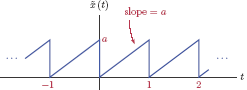
Example 4.8: Spectrum of periodic sawtooth waveform
Consider a periodic sawtooth signal , with a period of T0 = 1 s, defined by
and shown in Fig. 4.17. The parameter a is a real-valued constant. Determine the EFS coefficients for this signal.
Solution: The fundamental frequency of the signal is
Using Eqn. (4.72) we obtain
where we have used integration by parts. 2 Using Euler’s formula on Eqn. (4.78), real and imaginary parts of the EFS coefficients are obtained as
and
respectively. These two expressions can be greatly simplified by recognizing that sin (2πk) = 0 and cos(2πk) = 1 for all integers k. For k = 0, the values of Re{ck} and Im{ck} need to be resolved by using L’Hospital’s rule on Eqns. (4.79) and (4.80). Thus, the real and imaginary parts of ck are
Combining Eqns. (4.81) and (4.82) the magnitudes of the EFS coefficients are obtained as
For the phase angle we need to pay attention to the sign of the parameter a. If a ≥ 0, we have
If a < 0, then θk needs to be modified as
If a < 0, then θk needs to be modified as
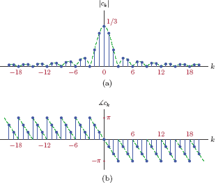
Magnitude and phase spectra for are graphed in Fig. 4.18(a) and (b) with the assumption that a > 0.

Line spectrum for the periodic sawtooth waveform of Example 4.8: (a) magnitude, (b) phase.
Software resources:
ex_4_8a.m
ex_4_8b.m
Example 4.9: Spectrum of multi-tone signal
Determine the EFS coefficients and graph the line spectrum for the multi-tone signal
shown in Fig. 4.19.
Solution: Using the appropriate trigonometric identity 3 the signal can be written as
Applying Euler’s formula, we have
By inspection of Eqn. (4.83) the significant EFS coefficients for the signal are found as
and all other coefficients are equal to zero. The resulting line spectrum is shown in Fig. 4.20.

Software resources:
ex_4_9.m
Example 4.10: Spectrum of half-wave rectified sinusoidal signal
Determine the EFS coefficients and graph the line spectrum for the half-wave periodic signal defined by
and shown in Fig. 4.21.

Solution: Using the analysis equation given by Eqn. (4.72), the EFS coefficients are
In order to simplify the evaluation of the integral in Eqn. (4.85) we will write the sine function using Euler’s formula, and obtain
which can be simplified to yield
We need to consider even and odd values of k separately.
Case 1: k odd and k ≠ ∓ 1
If k is odd, then both k − 1 and k + 1 are non-zero and even. We have e−jπ(k − 1) = e−jπ(k+1) = 1, and therefore ck = 0.
Case 2: k = 1
If k = 1, c1 has an indeterminate form which can be resolved through the use of L’Hospital’s rule:
Case 3: k = −1
Similar to the case of k = 1 an indeterminate form is obtained for k = −1. Through the use of L’Hospital’s rule the coefficient c−1 is found to be
Case 4: k even
In this case both k − 1 and k + 1 are odd, and we have e−jπ(k−1) = e−jπ(k+1) = −1.
Using this result in Eqn. (4.85) we get
Combining the results of the four cases, the EFS coefficients are
The resulting line spectrum is shown in Fig. 4.22.
Software resources:
ex 4_10a.m
ex_4_10b.m
4.2.4 Compact Fourier series (CFS)
Yet another form of the Fourier series representation of a periodic signal is the compact Fourier series (CFS) expressed as
Using the appropriate trigonometric identity 4 Eqn. (4.86) can be written as
Recognizing that this last equation for is in a format identical to the TFS expansion of the same signal given by Eqn. (4.26), the coefficients of the corresponding terms must be equal. Therefore the following must be true:
Solving for dk and ϕk from Eqns. (4.87), (4.88) and (4.89) we obtain
with d0 = a0, and ϕ0 = 0. CFS coefficients can also be obtained from the EFS coefficients by using Eqns. (4.88) and (4.89) in conjunction with Eqns. (4.60) and (4.61), and remembering that c−k = c*k for real-valued signals:
and
In the use of Eqn. (4.93), attention must be paid to the quadrant of the complex plane in which the coefficient ck resides.
Example 4.11: Compact Fourier series for a periodic pulse train
Determine the CFS coefficients for the periodic pulse train that was used in Example 4.6. Afterwards, using the CFS coefficients, find an approximation to using m = 4 harmonics.
Solution: CFS coefficients can be obtained from the EFS coefficients found in Example 4.6 along with Eqns. (4.92) and (4.93):
and
Table 4.3 lists values of some of the compact Fourier series coefficients for the pulse train x(t).
Compact Fourier series coefficients for the waveform in Example 4.11.
k |
dk |
ϕk (rad) |
|---|---|---|
0 |
0.3333 |
0.0000 |
1 |
0.5513 |
−1.0472 |
2 |
0.2757 |
−2.0944 |
3 |
0.0000 |
0.0000 |
4 |
0.1378 |
−1.0472 |
5 |
0.1103 |
−2.0944 |
6 |
0.0000 |
0.0000 |
7 |
0.0788 |
−1.0472 |
8 |
0.0689 |
−2.0944 |
9 |
0.0000 |
0.0000 |
10 |
0.0551 |
−1.0472 |
Let be an approximation to the signal utilizing the first m harmonics of the fundamental frequency, that is,
Using m = 4 and f0 = 1/3 Hz we have
The individual terms in Eqn. (4.95) as well as the resulting finite-harmonic approximation are shown in Fig. 4.23.

The contributing terms in Eqn. (4.95) and the the resulting finite-harmonic approximation.
4.2.5 Existence of Fourier series
For a specified periodic signal , one question that needs to be considered is the existence of the Fourier series: Is it always possible to determine the Fourier series coefficients? The answer is well-known in mathematics. A periodic signal can be uniquely expressed using sinusoidal basis functions at harmonic frequencies provided that the signal satisfies a set of conditions known as Dirichlet conditions named after the German mathematician Johann Peter Gustav Lejeune Dirichlet (1805–1859). A thorough mathematical treatment of Dirichlet conditions is beyond the scope of this text. For the purpose of the types of signals we will encounter in this text, however, it will suffice to summarize the three conditions as follows:
The signal must be integrable over one period in an absolute sense, that is
Any periodic signal in which the amplitude values are bounded will satisfy Eqn. (4.96). In addition, periodic repetitions of singularity functions such as a train of impulses repeated every T0 seconds will satisfy it as well.
If the signal has discontinuities, it must have at most a finite number of them in one period. Signals with an infinite number of discontinuities in one period cannot be expanded into Fourier series.
The signal must have at most a finite number of minima and maxima in one period. Signals with an infinite number of minima and maxima in one period cannot be expanded into Fourier series.
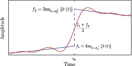
Most signals we encounter in engineering applications satisfy the existence criteria listed above. Consequently, they can be represented in series expansion forms given by Eqns. (4.26), (4.48) or (4.86). At points where the signal is continuous, its Fourier series expansion converges perfectly. At a point of discontinuity, however, the Fourier series expansion (TFS, EFS or CFS representation of the signal) yields the average value obtained by approaching the discontinuity from opposite directions. If the signal has a discontinuity at t = t0, and if {ck} are the EFS coefficients for it, we have
This is illustrated in Fig. 4.24.
4.2.6 Gibbs phenomenon
Let us further explore the issue of convergence of the Fourier series at a discontinuity. Consider the periodic square wave shown in Fig. 4.25.

The TFS coefficients of this signal were found in Example 4.4, and are repeated below:
Finite-harmonic approximation to the signal using m harmonics is
and the approximation error that occurs when m harmonics is used is
Several finite-harmonic approximations to are shown in Fig. 4.26 for m = 1, 3, 9, 25. The approximation error is also shown for each case.

Finite-harmonic approximations to a square-wave signal with period T0 = 2 s and the corresponding approximation errors.
We observe that the approximation error is non-uniform. It seems to be relatively large right before and right after a discontinuity, and it gets smaller as we move away from discontinuities. The Fourier series approximation overshoots the actual signal value at one side of each discontinuity, and undershoots it at the other side. The amount of overshoot or undershoot is about 9 percent of the height of the discontinuity, and cannot be reduced by increasing m. This is a form of the Gibbs phenomenon named after American scientist Josiah Willard Gibbs (1839-1903) who explained it in 1899. An enlarged view of the approximation and the error right around the discontinuity at t = 1 s are shown in Fig. 4.27 for m = 25. A further enlarged view of the approximation error corresponding to the shaded area in Fig. 4.27(b) is shown in Fig. 4.28. Notice that the positive and negative lobes around the discontinuity have amplitudes of about ±0.18 which is 9 percent of the amplitude of the discontinuity.

Enlarged view of the finite-harmonic approximation and the approximation error for m = 25.

One way to explain the reason for the Gibbs phenomenon would be to link it to the inability of sinusoidal basis functions that are continuous at every point to approximate a discontinuity in the signal.
4.2.7 Properties of Fourier series
Some fundamental properties of the Fourier series will be briefly explored in this section using the exponential (EFS) form of the series. A more thorough discussion of these properties will be given in Section 4.3.5 for the Fourier transform.
Linearity
For any two signals and periodic with T0 = 2π/ω0 and with their respective series expansions
and any two constants α1 and α2, it can be shown that the following relationship holds:
Linearity of the Fourier series:
Symmetry of Fourier series
Conjugate symmetry and conjugate antisymmetry properties were defined for discrete-time signals in Section 1.4.6 of Chapter 1. Same definitions apply to Fourier series coefficients as well. EFS coefficients ck are said to be conjugate symmetric if they satisfy
for all k. Similarly, the coefficients form a conjugate antisymmetric set if they satisfy
for all k.
If the signal is real-valued, it can be shown that its EFS coefficients form a conjugate symmetric set. Conversely, if the signal is purely imaginary, its EFS coefficients form a conjugate antisymmetric set.
Symmetry of Fourier series:
Polar form of EFS coefficients
Recall that the EFS coefficients can be written in polar form as
If the set {ck} is conjugate symmetric, the relationship in Eqn. (4.99) leads to
using the polar form of the coefficients. The consequences of Eqn. (4.104) are obtained by equating the magnitudes and the phases on both sides.
It was established in Eqn. (4.101) that the EFS coefficients of a real-valued are conjugate symmetric. Based on the results in Eqns. (4.105) and (4.106) the magnitude spectrum is an even function of k, and the phase spectrum is an odd function.
Similarly, if the set {ck} is conjugate antisymmetric, the relationship in Eqn. (4.100) reflects on polar form of ck as
The negative sign on the right side of Eqn. (4.107) needs to be incorporated into the phase since we could not write |c−k| = − |ck| (recall that magnitude must to be non-negative). Using e∓jπ = −1, Eqn. (4.107) becomes
The consequences of Eqn. (4.108) are summarized below.
Conjugate antisymmetric coefficients:
A purely imaginary signal leads to a set of EFS coefficients with conjugate antisymmetry. The corresponding magnitude spectrum is an even function of k as suggested by Eqn. (4.109). The phase is neither even nor odd.
Fourier series for even and odd signals
If the real-valued signal is an even function of time, the resulting EFS spectrum ck is real-valued for all k.
Conversely it can also be proven that, if the real-valued signal has odd-symmetry, the resulting EFS spectrum is purely imaginary.
Time shifting
For a signal with EFS expansion
it can be shown that
The consequence of time shifting is multiplication of its EFS coefficients by a complex exponential function of frequency.
4.3 Analysis of Non-Periodic Continuous-Time Signals
In Section 4.2 of this chapter we have discussed methods of representing periodic signals by means of harmonically related basis functions. The ability to express a periodic signal as a linear combination of standard basis functions allows us to use the superposition principle when such a signal is used as input to a linear and time-invariant system. We must also realize, however, that we often work with signals that are not necessarily periodic. We would like to have similar capability when we use non-periodic signals in conjunction with linear and time-invariant systems. In this section we will work on generalizing the results of the previous section to apply to signals that are not periodic. These efforts will lead us to the Fourier transform for continuous-time signals.
4.3.1 Fourier transform
In deriving the Fourier transform for non-periodic signals we will opt to take an intuitive approach at the expense of mathematical rigor. Our approach is to view a non-periodic signal as the limit case of a periodic one, and make use of the exponential Fourier series discussion of Section 4.2. Consider the non-periodic signal x(t) shown in Fig. 4.29.
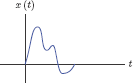
What frequencies are contained in this signal? What kind of a specific mixture of various frequencies needs to be assembled in order to construct this signal from a standard set of basis functions?
We already know how to represent periodic signals in the frequency domain. Let us construct a periodic extension of the signal x(t) by repeating it at intervals of T0.
This is illustrated in Fig. 4.30. The periodic extension can be expressed as a sum of time-shifted versions of x(t) shifted by all integer multiples of T0 to yield
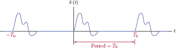
The selected period T0 should be sufficiently large so as not to change the shape of the signal by causing overlaps. Putting Eqn. (4.114) in summation form we obtain
Since is periodic, it can be analyzed in the frequency domain by using the methods developed in the previous section. The EFS representation of a periodic signal was given by Eqn. (4.71) which is repeated here:
The coefficients ck of the EFS expansion of the signal are computed as
We have used the starting point t0 = −T0/2 for the integral in Eqn. (4.116) so that the lower and upper integration limits are symmetric. Fundamental frequency is the reciprocal of the period, that is,
and the fundamental radian frequency is
Realizing that within the span −T0/2 < t < T0/2 of the integral, let us write Eqn. (4.116) as
If the period T0 is allowed to become very large, the periodic signal would start to look more and more similar to x(t). In the limit we would have
As the period T0 becomes very large, the fundamental frequency f0 becomes very small. In the limit, as we force T0 → ∞, the fundamental frequency becomes infinitesimal:
In Eqn. (4.118) we have switched to the notation Δf and Δω instead of f0 and ω0 to emphasize the infinitesimal nature of the fundamental frequency. Applying this change to the result in Eqn. (4.116) leads to
where ck is the contribution of the complex exponential at the frequency ω = k Δω. Because of the large T0 term appearing in the denominator of the right side of Eqn. (4.119), each individual coefficient ck is very small in magnitude, and in the limit we have ck → 0. In addition, successive harmonics k Δω are very close to each other due to infinitesimally small Δω. Let us multiply both sides of Eqn. (4.119) by T0 to obtain
If we now take the limit as T0 → ∞, and substitute ω = k Δω we obtain
The function X (ω) is the Fourier transform of the non-periodic signal x(t). It is a continuous function of frequency as opposed to the EFS line spectrum for a periodic signal that utilizes only integer multiples of a fundamental frequency. We can visualize this by imagining that each harmonic of the fundamental frequency comes closer and closer to its neighbors, finally closing the gaps and turning into a continuous function of ω.
At the start of the discussion it was assumed that the signal x(t) has finite duration. What if this is not the case? Would we be able to use the transform defined by Eqn. (4.121) with infinite-duration signals? The answer is yes, as long as the integral in Eqn. (4.121) converges.
Before discussing the conditions for the existence of the Fourier transform, we will address the following question: What does the transform X (ω) mean? In other words, how can we use the new function X (ω) for representing the signal x(t)? Recall that the Fourier series coefficients ck for a periodic signal were useful because we could construct the signal from them using Eqn. (4.116). Let us apply the limit operator to Eqn. (4.116):
If we multiply and divide the term inside the summation by T0 we obtain
and for large values of T0 we can write
In the limit, Eqn. (4.123) becomes
Also realizing that lim
and changing the summation to an integral in the limit we have
Eqn. (4.125) explains how the transform X (ω) can be used for constructing the signal x(t). We can interpret the integral in Eqn. (4.125) as a continuous sum of complex exponentials at harmonic frequencies that are infinitesimally close to each other. Thus, x(t) and X(ω) represent two different ways of looking at the same signal, one by observing the amplitude of the signal at each time instant and the other by considering the contribution of each frequency component to the signal.
In summary, we have derived a transform relationship between x(t) and X(ω) through the following equations:
Fourier transform for continuous-time signals:
Synthesis equation: (Inverse transform)
Analysis equation: (Forward transform)
Often we will use the Fourier transform operator ℱ and its inverse ℱ−1 in a shorthand notation as
for the forward transform, and
for the inverse transform. An even more compact notation for expressing the relationship between x (t) and X(ω) is in the form
In general, the Fourier transform, as computed by Eqn. (4.127), is a complex function of ω. It can be written in Cartesian complex form as
or in polar complex form as
Sometimes it will be more convenient to express the Fourier transform of a signal in terms of the frequency f in Hz rather than the radian frequency ω in rad/s. The conversion is straightforward by substituting ω = 2π f and d ω = 2π df in Eqns. (4.126) and (4.127) which leads to the following equations:
Fourier transform for continuous-time signals (using f instead of ω):
Synthesis equation: (Inverse transform)
Analysis equation: (Forward transform)
Note the lack of the scale factor 1/2π in front of the integral of the inverse transform when f is used. This is consistent with the relationship dω = 2π df.
4.3.2 Existence of Fourier transform
The Fourier transform integral given by Eqn. (4.127) may or may not converge for a given signal x(t). A complete theoretical study of convergence conditions is beyond the scope of this text, but we will provide a summary of the practical results that will be sufficient for our purposes. Let be defined as
and let ε (t) be the error defined as the difference between x (t) and :
For perfect convergence of the transform at all time instants, we would naturally want ε (t) = 0 for all t. However, this is not possible at time instants for which x (t) exhibits discontinuities. German mathematician Johann Peter Gustav Lejeune Dirichlet showed that the following set of conditions, referred to as Dirichlet conditions are sufficient for the convergence error ε (t) to be zero at all time instants except those that correspond to discontinuities of the signal x (t):
From a practical perspective, all signals we will encounter in our study of signals and systems will satisfy the second and third conditions regarding the number of discontinuities and the number of extrema respectively. The absolute integrability condition given by Eqn. (4.133) ensures that the result of the integral in Eqn. (4.126) is equal to the signal x (t) at all time instants except discontinuities. At points of discontinuities, Eqn. (4.126) yields the average value obtained by approaching the discontinuity from opposite directions. If the signal x (t) has a discontinuity at t = t0, we have
An alternative approach to the question of convergence is to require
which ensures that the normalized energy in the error signal ε (t) is zero even if the error signal itself is not equal to zero at all times. This condition ensures that the transform X (ω) as defined by Eqn. (4.127) is finite. It can be shown that, the condition stated by Eqn. (4.135) is satisfied provided that the signal x (t) is square integrable, that is
We have seen in Chapter 1 (see Eqn. (1.81)) that a signal that satisfies Eqn. (4.136) is referred to as an energy signal. Therefore, all energy signals have Fourier transforms. Furthermore, we can find Fourier transforms for some signals that do not satisfy Eqn. (4.136), such as periodic signals, if we are willing to accept the use of the impulse function in the transform. Another example of a signal that is not an energy signal is the unit-step function. It is neither absolute integrable nor square integrable. We will show, however, that a Fourier transform can be found for the unit-step function as well if we allow the use of the impulse function in the transform.
4.3.3 Developing further insight
The interpretation of the Fourier transform for a non-periodic signal as a generalization of the EFS representation of a periodic signal is fundamental. We will take the time to apply this idea step by step to an isolated pulse in order to develop further insight into the Fourier transform. Consider the signal x (t) shown in Fig. 4.31, an isolated rectangular pulse centered at t = 0 with amplitude A and width τ.

The analytical definition of x (t) is
Let the signal x (t) be extended into a pulse train with a period T0 as shown in Fig. 4.32.

By adapting the result found in Example 4.7 to the problem at hand, the EFS coefficients of the signal can be written as
where d is the duty cycle of the pulse train, and is given by
Substituting Eqn. (4.138) into Eqn. (4.137)
Let us multiply both sides of Eqn. (4.139) by T0 and write the scaled EFS coefficients as
where we have also substituted 1/T0 = f0 in the argument of the sinc function. The outline (or the envelope) of the scaled EFS coefficients ckT0 is a sinc function with a peak value of A τ at k = 0. The first zero crossing of the sinc-shaped envelope occurs at
which may or may not yield an integer result. Subsequent zero crossings occur for
or equivalently for
The coefficients ckT0 are graphed in Fig. 4.33(a) for A = 1, τ = 0.1 s and T0 = 0.25 s corresponding to a fundamental frequency of f0 = 4 Hz. Spectral lines for k = 1, k = 2 and k = 3 represent the strength of the frequency components at f0 = 4 Hz, 2f0 = 8 Hz and 3f0 = 12 Hz respectively. For the example values given, the first zero crossing of the sinc envelope occurs at k = 2.5, between the spectral lines for k = 2 and k = 3.
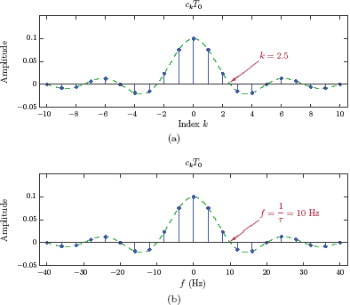
(a) The scaled line spectrum ckT0 for A = 1, τ = 0.1 s and T0 = 0.25 s, (b) the scaled line spectrum as a function of frequency f.
In Fig. 4.33(b) the same line spectrum is shown with actual frequencies f on the horizontal axis instead of the integer index k. The spectral line for index k now appears at the frequency f = kf0 = 4k Hz. For example, the spectral lines for k = 1, 2, 3 appear at frequencies f = 4, 8, 12 Hz respectively. The first zero crossing of the sinc envelope is at the frequency
and subsequent zero crossings appear at frequencies
What would happen if the period T0 is gradually increased while keeping the pulse amplitude A and the pulse width τ unchanged? The spectral lines in 4.33(b) are at integer multiples of the fundamental frequency f0. Since f0 = 1/T0, increasing the period T0 would cause f0 to become smaller, and the spectral lines to move inward, closer to each other. The zero crossings of the sinc envelope would not change, however, since the locations of the zero crossings depend on the pulse width τ only. Figs. 4.34(a)–(c) show the line spectra for T0 = 5, 10, 20 s respectively. In Fig. 4.34(a), the first zero crossing of the sinc envelope is still at 1/τ = 10 Hz, yet the frequency spacing of the spectral lines is now reduced to 2 Hz; therefore the first zero crossing coincides with the 5-th harmonic. In Fig. 4.34(b), the frequency spacing of the spectral lines is further reduced to 1 Hz and, consequently, the first zero crossing of the sinc envelope coincides with the 10-th harmonic, and is still at 10 Hz.

We can conclude that, as the period becomes infinitely large, the distances between adjacent spectral lines become infinitesimally small, and they eventually converge to a continuous function in the shape of the sinc envelope. It appears that the Fourier transform of the isolated pulse with amplitude A and width τ is
or, using the radian frequency variable ω,
Interactive Demo: ft_demo1.m
This demo program is based on the concepts introduced in the discussion above along with Figure. 4.31 Figure 4.32 Figure 4.33 Figure 4.34. The periodic pulse train with amplitude A, pulse width τ and period T0 is graphed. Its line spectrum based on the EFS coefficients is also shown. The spectrum graph includes the outline (or the envelope) of the EFS coefficients. Compare these graphs to Figs. 4.32 and 4.34. The amplitude is fixed at A = 5 since it is not a significant parameter for this demo. The period T0 and the pulse width τ may be varied by adjusting the slider controls, allowing us to duplicate the cases in Fig. 4.34.
- Increase the pulse period and observe the fundamental frequency change, causing the spectral lines of the line spectrum to move inward. Pay attention to how the outline remains fixed while this is occurring. Recall that the fundamental frequency is inversely proportional to the period; however, the outline is only a function of the pulse width.
- With the signal period fixed, increase the pulse width and observe the changes in the outline. Notice how the locations of the spectral lines remain unchanged, but the heights of the spectral lines get adjusted to conform to the new outline.
- For large values of the signal period observe how the outline approaches the Fourier transform of a single isolated pulse.
Software resources:
ft_demo1.m
4.3.4 Fourier transforms of some signals
In this section we will work on examples of determining the Fourier transforms of some fundamental signals.
Example 4.12: Fourier transform of a rectangular pulse
Using the forward Fourier transform integral in Eqn. (4.127), find the Fourier transform of the isolated rectangular pulse signal
shown in Fig. 4.35.

Solution: Recall that this is the same isolated pulse the Fourier transform of which was determined in Section 4.3.3 as the limit case of the EFS representation of a periodic pulse train. In this example we will take a more direct approach to obtain the same result through the use of the Fourier transform integral in Eqn. (4.127):
In order to use the sinc function, the result in Eqn. (4.144) can be manipulated and written in the form
In this case it will be easier to graph the transform in terms of the independent variable f instead of ω. Substituting ω = 2πf into Eqn. (4.46) we obtain
The spectrum X (f), shown in Fig. 4.36, is purely real owing to the fact that the signal x (t) exhibits even symmetry. The peak value of the spectrum is Aτ, and occurs at the frequency f = 0. The zero crossings of the spectrum occur at frequencies that satisfy fτ = k where k is any non-zero integer.

Software resources:
ex_4_12.m
The particular spectrum obtained in Example 4.12 is of special interest especially in digital systems. For example, in digital communications, rectangular pulses such as the one considered in Example 4.12 may be used for representing binary 0’s or 1’s. Let us observe the relationship between the pulse width and the shape of the spectrum:
- Largest values of the spectrum occur at frequencies close to f = 0. Thus, low frequencies seem to be the more significant ones in the spectrum, and the significance of frequency components seems to decrease as we move further away from f = 0 in either direction.
- The zero crossings of the spectrum occur for values of f that are integer multiples of 1/τ for multiplier values k = ±1, ±2,..., ±∞. As a result, if the pulse width is decreased, these zero crossings move further away from the frequency f = 0 resulting in the spectrum being stretched out in both directions. This increases the relative significance of large frequencies. Narrower pulses have frequency spectra that expand to higher frequencies.
- If the pulse width is increased, zero crossings of the spectrum move inward, that is, closer to the frequency f = 0 resulting in the spectrum being squeezed in from both directions. This decreases the significance of large frequencies, and causes the spectrum to be concentrated more heavily around the frequency f = 0. Wider pulses have frequency spectra that are more concentrated at low frequencies.
Fig. 4.37 illustrates the effects of changing the pulse width on the frequency spectrum.

Effects of changing the pulse width on the frequency spectrum: (a) A = 1 and τ = 1, (b) A = 2 and τ = 0.5, (c) A = 0.5 and τ = 2.
In all three cases illustrated in Fig. 4.37, the product of the pulse width and the pulse amplitude is fixed, i.e., Aτ = 1. Consequently, the peak of the frequency spectrum is equal to unity in each case. The placements of the zero crossings of the spectrum depend on the pulse width. In Fig. 4.37(a), the zero crossings are 1 Hz apart, consistent with the pulse width of τ = 1 s. In parts (b) and (c) of the figure, the spacing between adjacent zero crossings is 2 Hz and Hz, corresponding to pulse widths of τ = 0.5 s and τ = 2 s respectively.
This demo program is based on the concepts introduced in Example 4.12 and Figs. 4.35, 4.36, and 4.37. The amplitude A and the width τ of the rectangular pulse signal x(t) may be varied by using the two slider controls or by typing values into the corresponding edit fields. The Fourier transform X (f) is computed and graphed as the pulse parameters are varied.
- Pay particular attention to the relationship between the pulse width τ and the locations of the zero crossings of the spectrum.
- Observe how the concentrated nature of the spectrum changes as the pulse width is made narrower.
- Also observe how the height of the spectrum at f = 0 changes with pulse amplitude and pulse width.
Software resources:
ft_demo2.m
Example 4.13: Fourier transform of a rectangular pulse revisited
Using the forward Fourier transform integral in Eqn. (4.127), find the Fourier transform of the isolated rectangular pulse given by
which is shown in Fig. 4.38.

Solution: The signal x(t) is essentially a time-shifted version of the pulse signal used in Example 4.12. Using the Fourier transform integral in Eqn. (4.127) we obtain
At this point we will use a trick which will come in handy in similar situations in the rest of this text as well. Let us write the part of Eqn. (4.146) in square brackets as follows:
The use of Euler’s formula on the result of Eqn. (4.147) yields
Substituting Eqn. (4.148) into Eqn. (4.146), the Fourier transform of x(t) is found as
The transform found in Eqn. (4.149) is complex-valued, and is best expressed in polar form. In preparation for that, we will find it convenient to write the transform in terms of the frequency variable f through the substitution ω = 2πf:
We would ultimately like to express the transform of Eqn. (4.150) in the form
Let the functions B (f) and β (f) be defined as
and
so that
The functions B (f) and β (f) are shown in Fig. 4.39.
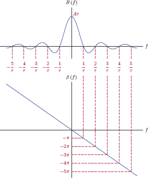
A quick glance at Fig. 4.39 reveals the reason that keeps us from declaring the functions B (f) and β (f) as the magnitude and the phase of the transform X (f): The function B (f) could be negative for some values of f, and therefore cannot be the magnitude of the transform. However, |X (ω)| can be writteninterms of B (f) by paying attention to its sign. In order to outline the procedure to be used, we will consider two separate example intervals of the frequency variable f:
Case 1: −1/τ < f < 1/τ
This is an example of a frequency interval in which B (f) ≥ 0, and
Therefore, we can write the transform as
resulting in the magnitude
and the phase
for the transform.
Case 2: 1/τ < f < 2/τ
For this interval we have B (f)< 0. The function B (f) can be expressed as
Using this form of B (f) in the transform leads to
which results in the magnitude
and the phase
for the transform X (f).
Comparison of the results in the two cases above leads us to the following generalized expressions for the magnitude and the phase of the transform X (f) as
In summary, for frequencies where B (f) is negative, we add ±π radians to the phase term to account for the factor (−1). This is illustrated in Fig. 4.40.

Phase values outside the interval (−π, π) radians are indistinguishable from the corresponding values within the interval since we can freely add any integer multiple of 2π radians to the phase. Because of this, it is customary to fit the phase values inside the interval (−π, π), a practice referred to as phase wrapping. Fig. 4.41 shows the phase characteristic after the application of phase wrapping.

ex_4_13.m
Example 4.14: Transform of the unit-impulse function
The unit-impulse function was defined in Section 1.3.2 of Chapter 1. The Fourier transform of the unit-impulse signal can be found by direct application of the Fourier transform integral along with the sifting property of the unit-impulse function.
In an effort to gain further insight, we will also take an alternative approach to determining the Fourier transform of the unit-impulse signal. Recall that in Section 1.3.2 we expressed the unit-impulse function as the limit case of a rectangular pulse with unit area. Given the pulse signal
the unit-impulse function can be expressed as
If the parameter a is gradually made smaller, the pulse q (t) becomes narrower and taller while still retaining unit area under it. In the limit, the pulse q (t) becomes the unit impulse function δ (t). Using the result obtained in Example 4.12 with A = 1/a and τ = a,the Fourier transform of q (t) is
Using an intuitive approach, we may also conclude that the Fourier transform of the unit-impulse function is an expanded, or stretched-out, version of the transform Q (f) in Eqn. (4.154), i.e.,
This conclusion is easy to justify from the general behavior of the function sinc (fa). Zero crossings on the frequency axis appear at values of f that are integer multiples of 1/a.As the value of the parameter a is reduced, the zero crossings of the sinc function move further apart, and the function stretches out or flattens around its peak at f = 0. In the limit, it approaches a constant of unity. This behavior is illustrated in Fig. 4.42.

Obtaining the Fourier transform of the unit-impulse signal from the transform of a rectangular pulse: (a) a = 2, (b) a = 1, (c) a = 0.2, (d) a = 0.1.
Interactive Demo: ft_demo3.m
The demo program “ft_demo3.m” illustrates the relationship between the Fourier transforms of the unit impulse and the rectangular pulse with unit area as discussed in the preceding section. A rectangular pulse with width equal to a and height equal to 1/a is shown along with its sinc-shaped Fourier transform. The pulse width may be varied through the use of a slider control. If we gradually reduce the width of the pulse, it starts to look more and more like a unit-impulse signal, and it becomes a unit-impulse signal in the limit. Intuitively it would make sense for the transform of the pulse to turn into the transform of the unit impulse. The demo program allows us to experiment with this concept.
- Start with a = 2 as in Fig. 4.42(a) and observe the spectrum of the pulse.
- Gradually reduce the pulse width and compare the spectrum to parts (b) through (d) of Fig. 4.42.
Software resources:
ft_demo3.m
Example 4.15: Fourier transform of a right-sided exponential signal
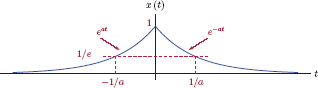
Determine the Fourier transform of the right-sided exponential signal
with a > 0 as shown in Fig. 4.43.

Solution: Application of the Fourier transform integral of Eqn. (4.127) to x (t) yields
Changing the lower limit of integral to t = 0 and dropping the factor u (t) results in
This result in Eqn. (4.155) is only valid for a > 0 since the integral could not have been evaluated otherwise. The magnitude and the phase of the transform are
Magnitude and phase characteristics are graphed in Fig. 4.44.

(a) The magnitude, and (b) the phase of the transform of the right-sided exponential signal in Example 4.15.
Some observations are in order: The magnitude of the transform is an even function of ω since
The peak magnitude occurs at ω = 0 and its value is |X (0)| = 1/a. At the radian frequency ω = a the magnitude is equal to which is times its peak value. On a logarithmic scale this corresponds to a drop of 3 decibels (dB). In contrast with the magnitude, the phase of the transform is an odd function of ω since
At frequencies ω → ±∞ the phase angle approaches
Furthermore, at frequencies ω = ±a the phase angle is
We will also compute real and imaginary parts of the transform to write its Cartesian form representation. Multiplying both the numerator and the denominator of the result in Eqn. (4.155) by (a − jω) we obtain
from which real and imaginary parts of the transform can be extracted as
respectively. Xr (ω) and Xi (ω) are shown in Fig. 4.45(a) and (b).

(a) Real part and (b) imaginary part of the transform of the right-sided exponential signal in Example 4.15.
In this case the real part is an even function of ω, and the imaginary part is an odd function.
Software resources:
ex_4_15a.m
ex_4_15b.m
Interactive Demo: ft_demo4.m
This demo program is based on Example 4.15. The right-sided exponential signal
and its Fourier transform are graphed. The parameter a may be modified through the use of a slider control.
Observe how changes in the parameter a affect the signal x (t) and the transform X (ω). Pay attention to the correlation between the width of the signal and the width of the transform. Does the fundamental relationship resemble the one observed earlier between the rectangular pulse and its Fourier transform?
Software resources:
ft_demo4.m
Example 4.16: Fourier transform of a two-sided exponential signal
Determine the Fourier transform of the two-sided exponential signal given by
where a is any non-negative real-valued constant. The signal x (t) is shown in Fig. 4.46.
Solution: Applying the Fourier transform integral of Eqn. (4.127) to our signal we get
Splitting the integral into two halves yields
Recognizing that
the transform is
X (ω) is shown in Fig. 4.47.

The transform X (ω) found in Eqn. (4.157) is purely real for all values of ω. This is a consequence of the signal x (t) having even symmetry, and will be explored further as we look at the symmetry properties of the Fourier transform in the next section. In addition to being purely real, the transform also happens to be non-negative in this case, resulting in a phase characteristic that is zero for all frequencies.
Software resources:
ex_4_16.m
Interactive Demo: ft_demo5.m
This demo program is based on Example 4.16. The two-sided exponential signal
and its Fourier transform are graphed. The transform is purely real for all ω owingtothe even symmetry of the signal x (t). The parameter a may be modified through the use of a slider control.
Observe how changes in the parameter a affect the signal x (t) and the transform X (ω). Pay attention to the correlation between the width of the signal and the width of the transform.
Software resources:
ft_demo5.m
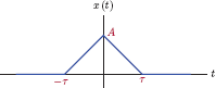
Example 4.17: Fourier transform of a triangular pulse
Find the Fourier transform of the triangular pulse signal given by
where Λ (t) is the unit-triangle function defined in Section 1.3.2 of Chapter 1. The signal x (t) is shown in Fig. 4.48.
Solution: Using the Fourier transform integral on the signal x (t), we obtain
The last two integrals in Eqn. (4.158) are similar in form to entry (B.16) of the table of indefinite integrals in Appendix B, repeated here for convenience:
Setting a = −jω results in
and the Fourier transform is
Using the appropriate trigonometric identity5 it can be shown that
It would be convenient to use the sinc function with the result in Eqn. (4.159). Recognizing that
the transform in Eqn. (4.159) can be written as
If the transform is written in terms of f instead of ω, we obtain
Thus, the Fourier transform of a triangular pulse is proportional the square of the sinc function. Contrast this with the Fourier transform of a rectangular pulse which is proportional to the sinc function as we have seen in Example 4.12. The transform of the triangular pulse, shown in Fig. 4.49, seems to be concentrated more heavily around low frequencies compared to the transform of the rectangular pulse.

We will have occasion to look at the transform of a triangular pulse in more depth when we study the properties of the Fourier transform in the next section. Specifically, a much simpler method of obtaining X (ω) for a triangular pulse will be presented after studying the convolution property of the Fourier transform.
Software resources:
ex_4_17.m
Interactive Demo: ft_demo6.m
This demo program is based on Example 4.17. The triangular pulse signal with peak amplitude A and width 2τ is shown along with its Fourier transform as determined in Eqn. (4.160). The transform is purely real for all f owing to the even symmetry of the triangular pulse signal x (t). The parameters A and τ may be modified through the use of slider controls.
Observe how parameter changes affect the signal x (t) and the transform X (ω). Pay attention to the correlation between the width of the signal and the width of the transform.
Software resources:
ft_demo6.m
Example 4.18: Fourier transform of the signum function
Determine the Fourier transform of the signum function defined as
and shown graphically in Fig. 4.50.

Solution: If we were to apply the Fourier transform integral directly to this signal, we would obtain
in which the two integrals cannot be evaluated. Instead, we will define an intermediate signal p (t) as
where a ≥ 0. We will first determine the Fourier transform of this intermediate signal, and then obtain the Fourier transform of the signum function from this intermediate result. The Fourier transform of p (t) is found as
The result is purely imaginary for all ω due to the odd symmetry of p (t). As the value of a is reduced, the intermediate signal p (t) starts to look more and more similar to the signum function, and becomes the signum function in the limit as a → 0. The transition of p (t) to sgn (t) is illustrated in Fig. 4.51 for a = 0.4, 0.15, and 0.04.

Signum function as a limit case of p (t) of Eqn. (4.161): (a)p (t) for a = 0.4 and its transform, (b)p (t) for a = 0.15 and its transform, (c)p (t) for a = 0.05 and its transform.
Setting a = 0 in the transform P (ω), we obtain the Fourier transform of the original signal x (t):
The magnitude of the transform is
and the phase is
Magnitude and phase characteristics are shown in Fig. 4.52.

Software resources:
ex_4_18.m
Interactive Demo: ft_demo7.m
This demo program is based on Example 4.18, and allows experimentation with the progression of the signal
and its corresponding Fourier transform P (ω) into the signal
and its associated transform X (ω) as the parameter a is made smaller. The parameter a may be adjusted through the use of a slider control. The program displays a graph of the signal p (t) and a graph of the imaginary part of transform P (ω). The real part of the transform is always equal to zero for this particular signal, and is therefore not shown.
Software resources:
ft_demo7.m
4.3.5 Properties of the Fourier transform
In this section we will explore some of the fundamental properties of the Fourier transform that provide further insight into its use for understanding and analyzing characteristics of signals. We will also see that some of these properties greatly simplify the computation of the Fourier transform for certain types of signals.
Linearity
Fourier transform is a linear operator. For any two signals x1 (t) and x2 (t) with their respective transforms
and any two constants α1 and α2, it can be shown that the following relationship holds:
Linearity of the Fourier transform:
Proof: Using the forward transform equation given by Eqn. (4.127) with the time domain signal [α1x1 (t) + α2x2 (t)] leads to:
Duality
Consider the transform pair
The transform relationship between x (t) and X (ω) is defined by the inverse and forward Fourier transform integrals given by Eqns. (4.126) and (4.127) and repeated here for convenience:
Suppose that we swap the roles of the independent variables to construct a new time-domain signal X (t) and a new frequency-domain function x (ω). What would be the relationship between X (t) and x (ω)?
The expressions for the inverse transform in Eqn. (4.126) and the forward transform in Eqn. (4.127) are interestingly similar. The main differences between the two integrals are the sign of the exponential term and the scale factor 1/2π for the analysis equation. This similarity leads to the duality principle of the Fourier transform. Let us change the integration variable of Eqn. (4.163) from ω to λ, and write it as
If ω →±∞ then λ →±∞, so we don’t need to change the limits of integration. Now, from a purely mathematical perspective, we will change the name of the independent variable from t to −ω, that is, we will evaluate the function on the left side of the integral in Eqn. (4.163) for t = −ω, and write the result as
Changing the integration variable from λ to t yields
and by multiplying both sides of Eqn. (4.165) by 2π we obtain
Eqn. (4.166) has the same general form as Eqn. (4.127) with substitutions x (t) → X (t) and X (ω) → 2πx (−ω). Thus, the following relationship must also be true:
The time-domain function X (t) and the frequency-domain function 2π x (−ω) form a Fourier transform pair. Thus, if X (ω) is the Fourier transform of x (t), then 2π x (−ω) is the Fourier transform of X (t).
Duality property:
We may find it more convenient to express the duality property using the frequency f instead of the radian frequency ω since this approach eliminates the 2π factor from the equations:
Duality property (using f instead of ω):
Duality property will be useful in deriving some of the other properties of the Fourier transform.
Example 4.19: Fourier transform of the sinc function
Find the Fourier transform of the signal
Solution: The Fourier transform of a rectangular pulse was found in Example 4.12 as a sinc function. Specifically we obtained
This relationship can be used as a starting point in finding the Fourier transform of x (t) = sinc (t). Let τ = 2π so that the argument of the sinc function in Eqn. (4.170) becomes ω:
In the next step, let A = 1/2π to obtain
Applying the duality property given by Eqn. (4.169) to the transform pair in Eqn. (4.172) leads to the result
Using f instead of ω in Eqn. (4.173) yields a relationship that is easier to remember:
The Fourier transform of x (t)= sinc(t) is a unit pulse in the frequency domain. The signal x (t) and its transform are graphed in Fig. 4.53(a) and (b).
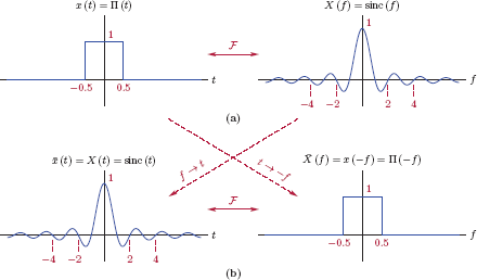
(a) The function x (t) = Π(t) and its Fourier transform X (f), (b) the function and its Fourier transform .
Example 4.20: Transform of a constant-amplitude signal
Find the Fourier transform of the constant-amplitude signal
Solution: Finding the Fourier transform of x (t) by direct application of Eqn. (4.127) is not possible since the resulting integral
could not be evaluated. On the other hand, in Example 4.14 we have concluded that the Fourier transform of the unit-impulse signal is a constant for all frequencies, that is
Applying the duality property to the transform pair in Eqn. (4.175) we obtain
If f is used instead of ω in the transform, then we have
This example also presents an opportunity for two important observations:
The signal x (t) = 1 does not satisfy the existence conditions discussed in Section 4.3.2; it is neither absolute integrable nor square integrable. Therefore, in a strict sense, its Fourier transform does not converge. By allowing the impulse function to be used in the transform, we obtain a function X (ω) that has the characteristics of a Fourier transform, and that can be used in solving problems in the frequency domain.
Sometimes we express the Fourier transform in terms of the radian frequency ω; at other times we use the frequency f. In general, the conversion from one format to another is just a matter of using the relationship ω = 2πf, so that
One exception to this rule is seen when the transform contains a singularity function. Compare Eqns. (4.176) and (4.176) in the example above.X (ω) has a 2π factor that X (f) does not have. This behavior is consistent with scaling of the impulse function (see Problem 1.6 of Chapter 1).
Example 4.21: Another example of using the duality property
Using the duality property, find the Fourier transform of the signal
which is graphed in Fig. 4.54.

Solution: While it is possible to solve this problem by a direct application of the Fourier transform integral given by Eqn. (4.127), it would be difficult to evaluate the integral unless we resort to the use of integration tables. Instead, we will simplify the solution by using another transform pair that we already know, and adapting that transform pair to our needs. In Example 4.16 wehavefound that
where the form of the transform bears a similarity to the time-domain expression for the signal x (t). In both functions the numerator is constant, and the denominator has a second-order term next to a constant term. We will make use of this similarity through the use of the duality property of the Fourier transform. The duality property allows us to write
as another valid transform pair. By taking steps that will preserve the validity of this transform pair, we will work toward making the time-domain component of the relationship in Eqn. (4.176) match the signal x (t) given in the problem statement. The signal x (t) has a 2t2 term in its denominator. Let us multiply both the numerator and the denominator of the time-domain component of Eqn. (4.176) by 2:
To match the constant term in the denominator of x (t) we will choose
and obtain
Afterwards, by scaling both sides of Eqn. (4.177) with we get
The transform found in Eqn. (4.178) is graphed in Fig. 4.55 using f as the independent variable instead of ω.
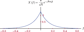
Software resources:
ex_4_21.m
Example 4.22: Signum function revisited
In Example 4.18 the Fourier transform of the signal x (t) = sgn(t) was found to be
Determine the time-domain signal, the Fourier transform of which is
Solution: This is another problem that could be simplified by the use of the duality property. Starting with the already known transform pair
and applying the duality property as expressed by Eqn. (4.168) we conclude that the following must also be a valid transform pair:
Recognizing that the sgn function has odd symmetry, that is, sgn (−ω) = −sgn(ω),
Multiplying both sides of Eqn. (4.178) by j/2π, we have
The signal we are seeking is
which is graphed in Fig. 4.56.
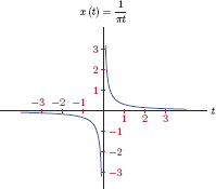
It is interesting to look at the magnitude and the phase of the transform X (ω) in Eqn. (4.178). The transform can be written as
Realizing that j = ejπ/2 we can write
The magnitude and the phase of X (ω) are shown in Fig. 4.57.

The magnitude of the transform is equal to unity for all frequencies. The phase of the transform is −π/2 radians for positive frequencies and +π/2 radians for negative frequencies.
Example 4.23: Fourier transform of the unit-step function
Determine the Fourier transform of the unit-step function x (t) = u (t).
Solution: The unit-step function does not satisfy the conditions for the existence of the Fourier transform. An attempt to find the transform by direct application of Eqn. (4.127) would result in
which does not converge. Instead, we will try to make use of some of the earlier results found along with the linearity property of the Fourier transform. The unit-step function can be expressed in terms of the signum function and a constant offset as
This is illustrated in Fig. 4.58.

Obtaining the unit-step function as the sum of the signum function and a constant offset.
Using the linearity of the Fourier transform we obtain
The transform of a constant signal was found in Example 4.20:
Furthermore, in Example 4.18 we found
Using these two results in Eqn. (4.180), Fourier transform of the unit-step function is
Fig. 4.59 shows the unit-step signal and the magnitude of its transform.

If the transform of the unit-step function is needed in terms of f instead of ω, the result in Eqn. (4.181) needs to be modified as
Symmetry of the Fourier Transform
Conjugate symmetry and conjugate antisymmetry properties were defined for time-domain signals in Section 1.3.6 of Chapter 1. Same definitions apply to a frequency-domain transform as well: A transform X (ω) is said to be conjugate symmetric if it satisfies
for all ω. Similarly, a transform X (ω) is said to be conjugate antisymmetric if it satisfies
for all ω. A transform does not have to be conjugate symmetric or conjugate antisymmetric. If it has any symmetry properties, however, they can be explored for simplifying the analysis in the frequency domain.
If the signal x (t) is real-valued,itcan be shown thatits Fourier transform X (ω) is conjugate symmetric. Conversely, if the signal x (t) is purely imaginary, its transform is conjugate antisymmetric.
Symmetry of the Fourier transform:
Proof:
Real x (t):
Let us begin by conjugating both sides of the forward transform integral given by Eqn. (4.127):
Since x (t) is real valued, x* (t) = x (t), and we have
In the next step we will derive X (−ω) from Eqn. (4.127) with the substitution ω → −ω:
Comparing Eqns. (4.188) and (4.189) we conclude that X* (ω) = X (−ω) when x (t) is real-valued.
Imaginary x (t):
In this case the complex conjugate of the transform is
since x* (t) = −x (t) for an imaginary signal. Comparison of Eqns. (4.189) and (4.190) leads to the conclusion that X* (ω) = −X (−ω) when x (t) is purely imaginary.
Cartesian and polar forms of the transform
A complex transform X (ω) can be written in polar form as
and in Cartesian form as
If X (ω) is conjugate symmetric, the relationship in Eqn. (4.183) can be written as
using the polar form of the transform, and
using its Cartesian form. The consequences of Eqns. (4.193) (4.194) can be obtained by equating the magnitudes and the phases on both sides of Eqn. (4.193) and by equating real and imaginary parts on both sides of Eqn. (4.194). The results can be summarized as follows:
Conjugate symmetric transform: X (−ω) = X* (ω)
We have already established the fact that the transform of a real-valued x (t) is conjugate symmetric. The results in Eqns. (4.195) and (4.196) suggest that, for such a transform, the magnitude is an even function of ω, and the phase is an odd function. Furthermore, based on Eqns. (4.197) and (4.198), the real part of the transform exhibits even symmetry while its imaginary part exhibits odd symmetry.
Similarly, if X (ω) is conjugate antisymmetric, the relationship in Eqn. (4.183) reflects on polar form of X (ω) as
The negative sign on the right side of Eqn. (4.199) needs to be incorporated into the phase sincewecould notwrite |X (−ω)| = −|X (ω)| (recall that magnitude needs to be a nonnegative function for all ω). Using e∓jπ = − 1, Eqn. (4.199) can be written as
Conjugate antisymmetry property of the transform can also be expressed in Cartesian form as
The consequences of Eqns. (4.199) and (4.201) are given below.
Conjugate antisymmetric transform: X (−ω) = −X* (ω)
A purely imaginary signal leads to a Fourier transform with conjugate antisymmetry. For such a transform the magnitude is still an even function of ω as suggested by Eqn. (4.202). The phase is neither even nor odd. The real part is an odd function of ω, and the imaginary part is an even function.
Example 4.24: Symmetry properties for the transform of right-sided exponential signal
The Fourier transform of the right-sided exponential signal x (t) = e−at u (t) was found in Example 4.15 to be
Elaborate on the symmetry properties of the transform.
Solution: Since the signal x (t) is real-valued, its transform must be conjugate-symmetric. The complex conjugate of the Fourier transform is
and the folded version of the transform, obtained by replacing ω with −ω in Eqn. (4.206), is
Thus we verify that X* (ω) = X (−ω), and the transform is conjugate symmetric. The magnitude and the phase of the transform are
respectively. We observe that the magnitude is an even function of frequency, that is,
consistent with the conclusion reached in Eqn. (4.195). On the other hand, the phase has odd symmetry since
consistent with Eqn. (4.196). By multiplying both the numerator and the denominator of the transform in Eqn. (4.206) by (a − jω) we have
Real and imaginary parts of the transform can be found as
and
It is atrivial matter to show that Xr (ω) is an even function of ω, and Xi (ω) is an odd function.
Software resources:
ex_4_24a.m
ex_4_24b.m
Transforms of even and odd signals
If the real-valued signal x (t) is an even function of time, the resulting transform X (ω) is real-valued for all ω.
Proof: If the imaginary part of the transform X (ω) is zero, then the transform must remain unchanged when it is conjugated. Thus, another way to express Eqn. (4.209) is by
This is the relationship we will prove. Let us conjugate both sides of the Fourier transform integral in Eqn. (4.127) to obtain
where we have used the fact that x* (t) = x (t) for a real-valued signal. Changing the integration variable from t to −λ, recognizing that dt = −dλ, and adjusting the integration limits accordingly we obtain
For a signal with even symmetry we have x (−λ) = x (λ), and the integral in Eqn. (4.212) becomes
Finally, swapping the two integration limits and negating the integral to compensate for it results in
Conversely it can also be proven that, if the real-valued signal x (t) has odd-symmetry, the resulting Fourier transform is purely imaginary. This can be mathematically stated as follows:
Conjugating a purely imaginary transform is equivalent to negating it, so an alternative method of expressing the relationship in Eqn. (4.215) is
The procedure for proving Eqn. (4.216) is very similar to the one given above for the transform of an even symmetric signal. (See Problem 4.25 at the end of this chapter.)
Example 4.25: Transform of a two-sided exponential signal
The two-sided exponential signal x (t) = e−a|t| was shown in Fig. 4.46, and has even symmetry. Its Fourier transform was found in Example 4.16 as
and was graphed in Fig. 4.47. As expected, the transform is real-valued for all ω.
Example 4.26: Transform of a pulse with odd symmetry
Consider the signal
shown in Fig. 4.60. Determine the Fourier transform X (ω) and show that it is purely imaginary.
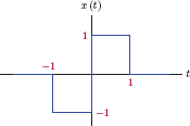
Solution: The transform can be found by direct use of the forward transform integral.
As expected, the transform is purely imaginary. Its magnitude, phase and imaginary part are graphed in Fig. 4.61.
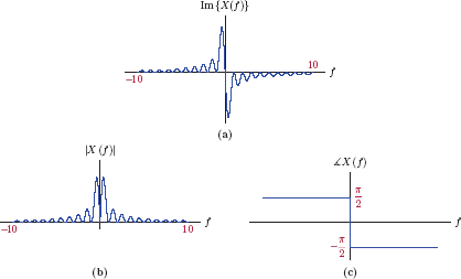
The Fourier transform found in Eqn. (4.217) for the odd symmetric pulse of Example 4.26: (a) imaginary part, (b) magnitude, (c) phase.
Software resources:
ex_4_26.m
Time shifting
Proof: Applying the Fourier transform integral in Eqn. (4.127) to x (t − τ) we obtain
Let λ = t − τ in the integral of Eqn. (4.219) so that
The exponential function in the integral of Eqn. (4.220) can be written as a product of two exponential functions to obtain
The consequence of shifting, or delaying, a signal in time is multiplication of its Fourier transform by a complex exponential function of frequency.
Example 4.27: Time shifting a rectangular pulse
The transform of a rectangular pulse with amplitude A, width τ and center at t = 0 was found in Example 4.12 as
In Example 4.13 the transform of a time shifted version of this pulse was determined by direct application of the Fourier transform integral as
The result in Eqn. (4.149) could easily have been obtained from the result in Eqn. (4.144) through the use of the time shifting property.
Example 4.28: Time shifting a two-sided exponential signal
Consider again the two-sided exponential signal used in earlier examples. A time shifted version of it is
The signal x (t) is shown in Fig 4.62 with the assumption that a > 0.
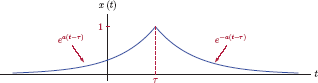
In Example 4.16 its Fourier transform was determined to be
Using the time shifting property of the Fourier transform we obtain
The transform X (ω) is shown in Fig. 4.63.
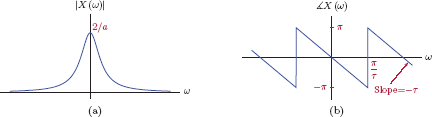
Transform of the time-shifted two-sided exponential signal of Example 4.28: (a) magnitude, (b) phase.
Compare this with the transform of the signal of Example 4.16. Note that time shifting the signal affects only the phase of the frequency spectrum, and not its magnitude.
Software resources:
ex_4_28.m
Frequency shifting
For a transform pair
it can be shown that
Proof: By directly applying the Fourier transform integral in Eqn. (4.127) to the signal x (t)e jω0t we obtain
An alternative proof can be obtained by using the duality principle in conjunction with the time shifting property. While it isn't necessarily shorter or simpler than the proof above, it nevertheless serves as another demonstration of the use of duality principle, and will therefore be given here. We start with the following two relationships:
If x (t) and X (ω) are a valid transform pair in Eqn. (4.224), then it follows through the use of the time-shifting property that Eqn. (4.225) is also valid. Applying the duality principle to each of the transform pairs in Eqns. (4.224) and (4.225) we obtain the following two relationships:
Let and . Also using the substitution ω0 = −τ, the two transforms in Eqns. (4.226) and (4.227) can be rewritten as
Modulation property
Modulation property is an interesting consequence of the frequency shifting property combined with the linearity of the Fourier transform. As its name implies, it finds significant use in modulation techniques utilized in analog and digital communications. We will have the occasion to use it when we study amplitude modulation in Chapter 11.
For a transform pair
it can be shown that
and
Multiplication of a signal by a cosine waveform causes its spectrum to be shifted in both directions by the frequency of the cosine waveform, and to be scaled by ½. Multiplication of the signal by a sine waveform causes a similar effect with an added phase shift of −π/2 radians for positive frequencies and π/2 radians for negative frequencies.
Proof: Using Euler's formula, the left side of the relationship in Eqn. (4.230) can be written as
The desired proof is obtained by applying the frequency shifting property to the terms on the right side of Eqn. (4.232). Using Eqn. (4.222) we obtain
and
which could be used together in Eqn. (4.232) to arrive at the result in Eqn. (4.230).
The proof of Eqn. (4.231) is similar, but requires one additional step. Again using Euler's formula, let us write the left side of Eqn. (4.231) as
Realizing that
Eqn. (4.235) can be rewritten as
The proof of Eqn. (4.231) can be completed by using Eqns. (4.233) and (4.234) on the right side of Eqn. (4.236).
Find the Fourier transform of the modulated pulse given by
Solution: Let p (t) be defined as a rectangular pulse centered around the time origin with a pulse width of 2τ and a unit amplitude, i.e.,
Using p (t), the signal x (t) can be expressed in a more compact form as
This is illustrated in Fig. 4.64.
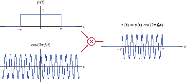
Expressing the modulated pulse signal of Example 4.29 as the product of a rectangular pulse and a sinusoidal signal.
The transform of the pulse p (t) is
We will apply the modulation property to this result to obtain the transform we seek:
Construction of this spectrum is illustrated in Fig. 4.65.

Transform of the modulated pulse of Example 4.29 obtained by adding frequency-shifted versions of P (ω).
ex_4_29.m
Interactive Demo: ft_demo8.m
This demo program is based on Example 4.29. It allows experimentation with modulated pulse signal and its Fourier transform. Pulse width parameter τ and the frequency f0 may be varied using slider controls. Both the modulated pulse signal and its transform are graphed.
- What is the effect of changing the pulse width on the spectrum?
- How does the frequency f0 affect the shape of the spectrum?
Software resources:
ft_demo8.m
Time and frequency scaling
For a transform pair
it can be shown that
The parameter a is any non-zero and real-valued constant.
Proof: The Fourier transform of x (at) is
A new independent variable λ will be introduced through the variable change at = λ. Let us substitute
in the integral of Eqn. (4.241). We need to consider the cases of a> 0and a < 0 separately. If a > 0, then t → ±∞ implies λ → ±∞. Therefore, the limits of the integral remain unchanged under the variable change, and we have
If a < 0, however, the same substitution leads to
since t → ±∞ now leads to λ → ∓∞. Swapping the lower and upper limits of the integral and negating the result to compensate for it yields
It is possible to combine Eqns. (4.242) and (4.244) into one compact expression by letting the scale factor in front of the integral be expressed as 1/|a| so that it is valid for both a > 0 and a < 0. Thus we obtain the desired proof:
This property is significant in signal processing. The implication of Eqn. (4.239) is that, if the time variable is scaled by a factor a, the frequency variable is scaled by the same factor, but in the opposite direction.
Example 4.30: Working with scaled and shifted pulses
Determine the Fourier transform of the signal
which is shown in Fig 4.66.

Solution: It certainly is possible to use the Fourier transform integral of Eqn. (4.127) directly on the signal x (t). It would be more convenient, however, to make use of the properties of the Fourier transform. The signal x (t) can be written as the sum of two rectangular pulses:
- One with amplitude of A1 = −1, width τ1 = 2 s, center at td1 = 0.5s
- One with amplitude of A2 = 0.75, width τ2 = 4 s, center at td2 = 3.5
Using the unit-pulse function Π (t) we have
The Fourier transform of the unit-pulse function is
Using the scaling property of the Fourier transform, the following two relationships can be written:
In addition, the use of the time-shifting property leads to
Using Eqns. (4.246) and (4.247) the Fourier transform of x (t) is
which is graphed in Fig. 4.67.

Software resources:
ex_4_30.m
The demo program “fd_demo9.m” is based on Example 4.30. It illustrates the use of time scaling and time shifting properties of the Fourier transform for computing the transform of a signal that can be expressed as the sum of two rectangular pulses. The signal to be constructed is in the form
Parameters A1, A2, τ1 τ2, td1 and td2 can be varied using slider controls. The individual spectrum of each pulse is displayed along with the spectrum of the signal x (t).
Software resources:
fd_demo9.m
Differentiation in the time domain
Proof: We will first prove the relationship in Eqn. (4.248) for n = 1. Once this is done, proof for n > 1 is easily obtained by repeating the process. The proof for Eqn. (4.249) is very similar, and will be left as an exercise (see Problem 4.28 at the end of this chapter).
Consider the inverse Fourier transform relationship given by Eqn. (4.126). Differentiating both sides of it with respect to t yields
Swapping the order of differentiation and integration on the right side of Eqn. (4.250) we can write
which leads us to the conclusion
Thus, differentiation of the signal with respect to the time variable corresponds to multiplication of the transform with jω. Differentiating both sides of Eqn. (4.251) one more time yields
or in compact form
It is obvious that each differentiation of the signal x (t) will bring up another (jω) factor in the corresponding transform. Differentiating the signal x (t) for n times corresponds to multiplying the transform by (jω)n.
Example 4.31: Triangular pulse revisited
Recall that the Fourier transform of the triangular pulse signal
was found in Example 4.17 through direct application of the Fourier transform integral of Eqn. (4.127). Rework the problem using the differentiation-in-time property.
Solution: Instead of working with the signal x (t) directly, we will find it convenient to work with its derivative
shown in Fig. 4.68.

Using the unit-pulse function along with time-scaling and time-shifting operations, w (t) can be expressed as
Using the variable f instead of ω for convenience, the transform W (f) can be computed from Eqn. (4.255) as
The real part of W (f) is equal to zero; its imaginary part is shown in Fig. 4.69. Frequency-domain equivalent of the relationship in Eqn. (4.256) is
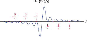
Solving Eqn. (4.257) for X (f) yields
which is in agreement with the answer found in Example 4.17.
Example 4.32: Fourier transform of a trapezoidal pulse
Determine the Fourier transform of the trapezoidal pulse x (t) shown in Fig. 4.70
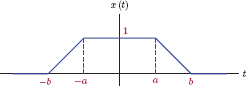
Solution: Analytical description of this signal could be given in the form
Once again we will use the intermediate signal w (t) obtained by differentiating x (t) with respect to t:
The signal w (t) is shown in Fig. 4.71.

Finding the Fourier transform of w (t) is much easier compared to a direct evaluation of the Fourier transform integral for x (t). For notational convenience, let two new parameters be defined as
The parameter τ is the width of each of the two pulses that make up w (t), and these pulses are centered at ±λ. The derivative w (t) can be written using the unit-pulse function as
and the corresponding transform W (f) is
The transform of x (t) can now be found by scaling this result:
The transform X (f) is graphed in Fig. 4.72 for various values of the parameters τ and λ.

Having found the solution for X (f) we will speculate on the differentiation in time property a bit further. What if we had differentiated w (t) one more time to obtain a new signal v (t)? Let
The signal v (t) consists of some shifted and scaled impulses, and is shown in Fig. 4.73.

The transform of v (t) would be related to the transform of x (t) by
Analytically, v (t) can be expressed as
Knowing that ℱ{δ(t)} = 1, and utilizing the time-shifting property of the Fourier transform, V (f) is found to be
Based on Eqn. (4.258), we have
Substituting a and b into Eqn. (4.261) we obtain
Using the appropriate trigonometric identity,6 Eqn. (4.262) becomes
and the transform X (f) is obtained by using Eqn. (4.260) as
which matches the result found earlier.
ex_4_32.m
Interactive Demo: fd_demo10
The demo program “fd_demo10.m” illustrates the steps involved in Example 4.32 for finding the Fourier transform of a trapezoidal pulse through the use of the differentiation in time property. The signals x (t) and w (t) are displayed on the left side of the graphical user interface window. On the right, the transforms are displayed. The parameters τ and λ may be adjusted using the two slider controls provided. Based on Eqn. (4.259) the real part of W (f) is zero, and therefore only its imaginary part is shown. On the other hand, the transform X (f) is purely real as given by Eqn. (4.260). We graph X (f)/λ so that the peak magnitude of the resulting graph is fixed, and we can concentrate on the placement of zero crossings as the parameters τ and λ are varied.
It is also interesting to note that, for λ = τ/2, the trapezoidal pulse x (t) becomes identical to the triangular pulse of Example 4.31. In the demo program it is possible to see this by setting λ = 0.5 and τ = 1. The corresponding transforms W (f) and X (f)/λ should also agree with the results of Example 4.31.
Software resources:
fd_demo10.m
Differentiation in the frequency domain
For a transform pair
it can be shown that
If we choose to use f instead or ω, then
Proof: The proof is straightforward and is similar to the proof of Eqn. (4.248). It will be carried out for Eqn. (4.264). The very similar proof of Eqn. (4.265) will be left as an exercise (see Problems 4.29 and 4.30 at the end of this chapter).
Let us differentiate both sides of the Fourier transform integral in Eqn. (4.127) with respect to ω:
Changing the order of integration and differentiation on the right side of Eqn. (4.266) yields
to prove Eqn. (4.264) for n = 1. Proof for n> 1 can easily be obtained by repeated use of this procedure.
Alternatively, we might see the similarity between the expressions of the differentiation properties in time and frequency domains, and prove the latter from the knowledge of the former through the use of the duality principle. Let's start with the following two relationships:
If x (t) and X (f) are a valid transform pair in Eqn. (4.268), then Eqn. (4.269) is also valid by the differentiation in time property. Application of the duality principle to each of the transform pairs in Eqns. (4.268) and (4.269) leads to the following two relationships:
Let and . The two transforms in Eqns. (4.270) and (4.271) can be rewritten as
Finally, multiplication of both sides of the transform pair in Eqn. (4.273) by (−1)n yields
which completes the proof. If Eqn. (4.272) represents a valid transform pair, then so does Eqn. (4.274).
Example 4.33: Pulse with trapezoidal spectrum
Find the signal x (t) the Fourier transform of which is the trapezoidal function given by
and shown in Fig. 4.74. Real-valued parameter r is adjustable in the range 0 < r < 1.

Solution: The answer can easily be found by applying the duality property to the result obtained in Eqn. (4.259) of Example 4.32 with the adjustments a = f0 (1 − r), b = f0 (1 + r), λ = f0 and τ =2f0r. (See Problem 4.32 at the end of this chapter.) Instead of using that approach, however, we will use this example as an opportunity to apply the differentiation in frequency property. Let
By carrying out the differentiation we obtain W (f) as
which is shown in Fig. 4.75.

The Fourier transform of the sinc function is (see Example 4.19)
Using the time and frequency scaling property of the Fourier transform given by Eqn. (4.239) we obtain
The two frequency-domain pulses that make up the transform W (f) are simply frequency shifted and frequency scaled versions of the right side of Eqn. (4.275). Therefore, the inverse
Since w (t) = −j2πt x (t), we can write x (t) as
Fig. 4.76 shows the signal x (t) for various values of the parameter r.

The time-domain signal x (t) with the trapezoidal spectrum X (f) used in Example 4.33: (a) r = 0.1, (b) r = 0.4, (c) r = 0.7.
The signal x (t) with a trapezoidal spectrum exhibits some interesting properties:
- Zero crossings of the signal x (t) occur at uniform time intervals of 1/(2f0) regardless of the value of r.
- Larger values of r result in a reduction in the oscillatory behavior of the signal.
These properties are very significant in communication systems in the context of pulse shaping. A signal with the properties listed above can be used for representing binary or M-ary symbols while eliminating the interference of those symbols with each other, a phenomenon known as intersymbol interference (ISI). Harry Nyquist has shown that any signal the spectrum of which has certain symmetry properties will exhibit uniformly spaced zero crossings. The trapezoidal spectrum shown in Fig. 4.74 is one example.
ex_4_33.m
Interactive Demo: ft_demo11
The demo program “ft_demo11.m” expands on the concepts explored in Example 4.33. The trapezoidal spectrum X (f) with parameters f0 and r and its corresponding time-domain signal x (t) are shown. Values of parameters f0 and r may be adjusted using slider controls. The zero crossings of the signal x (t) are shown with marker lines. Specifically observe the following:
- As the parameter f0 is changed, the zero crossings of the signal coincide with integer multiples of 1/(2f0). (You may need to zoom in to observe that zero crossings are always uniformly spaced.)
- Vary the parameter r and observe its effect on the locations of zero crossings. Does it seem to have an effect?
- The one-sided bandwidth of the trapezoidal spectrum is f0 (1 +r). If f0 is fixed, bandwidth can be controlled by the parameter r. Observe the effect of increasing the bandwidth of the spectrum on the shape of the signal x (t).
Software resources:
ft_demo11.m
Convolution property
For two transform pairs
it can be shown that
Proof: The proof is obtained by direct application of the Fourier transform integral in Eqn. (4.127) to the convolution of signals x1 (t) and x2 (t):
Interchanging the order of two integrals and rearranging terms we obtain
In Eqn. (4.280), we will recognize the expression in square brackets as the Fourier transform of the time shifted signal x2 (t − λ). The use of time shifting property of the Fourier transform given by Eqn. (4.218) yields
Substituting Eqn. (4.281) into Eqn. (4.280) we get
Multiplication of two signals
For two transform pairs
it can be shown that
If we choose to use f instead of ω, then
Proof: The right side of Eqn. (4.284) can be written as
Applying the inverse Fourier transform to both sides of Eqn. (4.286) yields
Changing the order of the two integrals on the right side of Eqn. (4.287), and arranging terms, we obtain
Recall from the frequency shifting property of the Fourier transform, given by Eqn. (4.222), that X2 (ω − λ) is the Fourier transform of the signal x2 (t) multiplied by a complex exponential. The expression in square brackets on the right side of Eqn. (4.288) represents the inverse Fourier transform of X2 (ω − λ), and evaluates to
Substituting Eqn. (4.289) into Eqn. (4.288) and rearranging the terms on the right side, we have
Example 4.34: Transform of a truncated sinusoidal signal
A sinusoidal signal that is time-limited in the interval −τ< t < τ is given by
Determine the Fourier transform of this signal using the multiplication property.
Solution: The signal x (t) is the same as the modulated pulse signal used in Example 4.29 and shown in Fig. 4.64. In Example 4.29 the transform was determined using the modulation property. Let x1 (t) and x2 (t) be defined as
The signal x (t) can be written as the product of these two signals:
It will be more convenient to use f rather than ω in this case. Fourier transforms of the signals x1 (t) and x2 (t) are
and
respectively. Using Eqn. (4.285), the Fourier transform of the product x (t) = x1 (t) x2 (t) is
which matches the result found in Example 4.29.
Software resources:
ex_4_34.m
Interactive Demo: ft_demol2
The demo program “ft_demol2.m” is based on Example 4.34, and illustrates the multiplication property of the Fourier transform. On the left side of the screen, the signals xi (t) and x2 (t) of Example 4.34 as well as their product [xi (t) x2 (t)] are graphed. The right side of the screen displays the corresponding spectra X1 (f), X2 (f), and [Xi (f) * X2 (f)]. Parameters τ and f0 may be adjusted using slider controls.
Software resources:
ft_demol2.m
Integration
For a transform pair
it can be shown that
Proof: Recall that in Example 4.23 we have found the Fourier transform of a unit-step function to be
Now consider the convolution of the signal x(t) with a unit-step signal, i.e.,
We know that
Using Eqn. (4.294) to modify the integration limits in Eqn. (4.293) we obtain
The right side of Eqn. (4.295) is the function the Fourier transform of which we are seeking. We also know from Eqn. (4.279) that
Thus we have
Using the sampling property of the impulse function, Eqn. (4.297) becomes
Table 4.4 contains a summary of key properties of the Fourier transform. Table 4.5 lists some of the fundamental Fourier transform pairs.
Fourier transform properties.
Property |
Signal |
Transform |
|---|---|---|
Linearity |
α x1 (t) + β x2 (t) |
α X1 (ω) + β X2 (ω) |
Duality |
X (t) |
2 π x (−ω) |
Conjugate symmetry |
x (t) real |
|
Conjugate antisymmetry |
x (t) imaginary |
|
Even signal |
x (−t) = x (t) |
Im {X (ω)} = 0 |
Odd signal |
x (−t) = −x (t) |
Re {X (ω)} = 0 |
Time shifting |
x (t − τ) |
X (ω) e−jωτ |
Frequency shifting |
x (t) eejω0t |
X (ω − ω0) |
Modulation property |
x (t) cos(ω0t) |
|
Time and frequency scaling |
x (at) |
|
Differentiation in time |
(jω)n X (ω) |
|
Differentiation in frequency |
(−jt)n x (t) |
|
Convolution |
x1 (t) * x2 (t) |
|
Multiplication |
x1 (t) x2 (t) |
|
Integration |
||
Parseval's theorem |
||
Some Fourier transform pairs.
Signal |
Transform |
|
|---|---|---|
Rectangular pulse |
x (t) = AΠ (t/τ) |
|
Triangular pulse |
x (t) = A Λ (t/τ) |
|
Right-sided exponential |
x (t) = e−at u(t) |
|
Two-sided exponential |
x (t) = e−a|t| |
|
Signum function |
x (t) = sgn (t) |
|
Unit impulse |
x (t) = δ(t) |
|
Sinc function |
x (t) = sinc(t) |
|
Constant-amplitude signal |
x (t) = 1, all t |
X (ω) = 2π δ(ω) |
|
X (ω) = −j sgn(ω) |
|
Unit-step function |
x (t) = u(t) |
|
Modulated pulse |
4.3.6 Applying Fourier transform to periodic signals
In developing frequency-domain analysis methods in the previous sections of this chapter we have distinguished between periodic and non-periodic continuous-time signals. Periodic signals were analyzed using various forms of the Fourier series such as TFS, EFS or CFS. In contrast, Fourier transform was used for analyzing non-periodic signals. While this distinction will be appropriate when we work with one type of signal or the other, there may be times when we need to mix periodic and non-periodic signals within the same system. An example of this occurs in amplitude modulation where a non-periodic message signal may be multiplied with a periodic carrier signal. Another example is the use of a periodic signal as input to a system the impulse response of which is non-periodic. In such situations it would be convenient to use the Fourier transform for periodic signals as well. In general a periodic signal is a power signal that does not satisfy the existence conditions for the Fourier transform. It is neither absolute integrable nor square integrable. On the other hand, we have seen in Example 4.20 that a Fourier transform can be found for a constant-amplitude signal that does not satisfy the existence conditions, as long as we are willing to accept singularity functions in the transform. The next two examples will expand on this idea. Afterwards we will develop a technique for converting the EFS representation of a periodic continuous-time signal to a Fourier transform that is suitable for use in solving problems.
Example 4.35: Fourier transform of complex exponential signal
Determine the transform of the complex exponential signal x (t) = e jωot.
Solution: The transform of the constant unit-amplitude signal was found in Example 4.20 to be
Using this result along with the frequency shifting property of the Fourier transform given by Eqn. (4.222), the transform of the complex exponential signal is
This is illustrated in Fig. 4.77.

Example 4.36: Fourier transform of sinusoidal signal
Determine the transform of the sinusoidal signal x(t) = cos (ω0t).
Solution: The transform of the constant unit-amplitude signal was found in Example 4.20 to be
Using this result along with the modulation property of the Fourier transform given by Eqn. (4.230), the transform of the sinusoidal signal is
This transform is shown in Fig. 4.78.
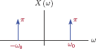
In Examples 4.35 and 4.36 we were able to obtain the Fourier transforms of two periodic signals, namely a complex exponential signal and a sinusoidal signal. Both transforms were possible through the use of impulse functions in the transform. The idea can be generalized to apply to any periodic continuous-time signal that has an EFS representation.
The EFS synthesis equation for a periodic signal was given by Eqn. (4.71) which is repeated here for convenience:
Using the Fourier transform analysis equation given by Eqn. (4.127), the transform of is
Interchanging the order of the integral and the summation in Eqn. (4.301) and rearranging terms we obtain
In Eqn. (4.303) the expression in square brackets is the Fourier transform of the signal ejkω0t which, using the result obtained in Example 4.35, can be written as
Using Eqn. (4.304) in Eqn. (4.303), the transform of the periodic signal with EFS coefficients {ck} is obtained as
The Fourier transform for a periodic continuous-time signal is obtained by converting each EFS coefficient ck to an impulse with area equal to 2πck and placing it at the radian frequency ω = kω0. This process is illustrated in Fig. 4.79.

(a) EFS coefficients for a signal , (b) Fourier transform obtained through Eqn. (4.305).
Example 4.37: Fourier transform of periodic pulse train
Determine the Fourier transform of the periodic pulse train with duty cycle d = τ/T0 as shown in Fig. 4.80.
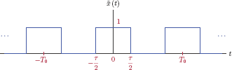
Solution: The EFS coefficients for were determined in Example 4.7 as
Using Eqn. 4.305 the Fourier transform is
where ω0 = 1/T0 is the fundamental radian frequency.
4.4 Energy and Power in the Frequency Domain
In this section we will discuss a very important theorem of Fourier series and transform known as Parseval’s theorem which can be used as the basis of computing energy or power of a signal from its frequency domain representation. Afterwards energy and power spectral density concepts will be introduced.
4.4.1 Parseval’s theorem
For a periodic power signal with period of T0 and EFS coefficients {ck} it can be shown that
For a non-periodic energy signal x(t) with a Fourier transform X (f), the following holds true:
The left side of Eqn. (4.307) represents the normalized average power in a periodic signal as we have derived in Eqn. (1.92). The left side of Eqn. (4.308) represents the normalized signal energy as derived in Eqn. (1.81). The relationships given by Eqns. (4.307) and (4.308) relate signal energy or signal power to the frequency-domain representation of the signal. They are two forms of Parseval’s theorem.
Proofs: We will begin with the proof of Eqn. (4.307). We know from Eqn. (4.48) that
The left side of Eqn. (4.307) can be written as
By rearranging the order of the two summations and the integral in Eqn. (4.310), we have
Using orthogonality of exponential basis functions (see Eqn. (4.63)), we have
As a result, the inner summation in Eqn. (4.311) evaluates to T0, and we have
which proves Eqn. (4.307). The proof for Eqn. (4.308) is quite similar. We know that for an energy signal x (t) the inverse Fourier transform equation is
The normalized energy of x (t) can be written as
By interchanging the order of the two integrals in Eqn. (4.313) and rearranging terms we get
which proves Eqn. (4.308).
4.4.2 Energy and power spectral density
Examining the two statements of Parseval’s theorem expressed by Eqns. (4.307) and (4.308), we reach the following conclusions:
In Eqn. (4.307) the left side corresponds to the normalized average power of the signal , and therefore the summation on the right side must also represent power. The term |ck|2 corresponds to the power of the frequency component at f = kf0, thatis, the power in the k-th harmonic only. Suppose we construct a new function Sx (f) by starting with the line spectrum ck and replacing each spectral line with an impulse function scaled by |ck|2 and time shifted to the frequency kf0, i.e.,
In the next step we will integrate Sx (f) to obtain
Using the sifting property of the unit-impulse function Eqn. (4.316) becomes
Finally, substituting Eqn. (4.317) into Eqn. (4.307) we have
In Eqn. (4.318) the normalized average power of the signal x (t) is computed by integrating the function Sx (f) over all frequencies. Consequently, the function Sx (f) is the power spectral density of the signal x (t).
If we use the radian frequency variable ω instead of f, Eqn. (4.318) becomes
As an interesting by-product of Eqn. (4.318), the power of x (t) thatis withina specific frequency range can be determined by integrating Sx (f) over that frequency range. For example, the power contained at frequencies in the range (−f0, f0) can be computed as
In Eqn. (4.308) the left side is the normalized signal energy for the signal x (t), and the right side must be the same. The integrand |X (f)|2 is therefore the energy spectral density of the signal x (t). Let the function Gx (f) be defined as
Substituting Eqn. (4.321) into Eqn. (4.308), the normalized energy in the signal x (t) can be expressed as
If ω is used in place of f, Eqn. (4.322) becomes
In Eqn. (4.308) we have expressed Parseval’s theorem for an energy signal, and used it to lead to the derivation of the energy spectral density in Eqn. (4.321). We know that some non-periodic signals are power signals, therefore their energy cannot be computed. The example of one such signal is the unit-step function. The power of a non-periodic signal was defined in Eqn. (1.93) which will be repeated here:
In order to write the counterpart of Eqn. (4.308) for a power signal, we will first define a truncated version of x (t) as
Let XT(f) be the Fourier transform of the truncated signal XT(t):
Now Eqn. (4.308) can be written in terms of the truncated signal and its transform as
Scaling both sides of Eqn. (4.324) by (1/T) and taking the limit as T becomes infinitely large, we obtain
The left side of Eqn. (4.325) is the average normalized power in a non-periodic signal as we have established in Eqn. (1.93). Therefore, the power spectral density of x(t) is
Example 4.38: Power spectral density of a periodic pulse train
The EFS coefficients for the periodic pulse train shown in Fig. 4.81 were found in Example 4.5 to be

Determine the power spectral density for . Also find the total power, the dc power, the power in the first three harmonics, and the power above 1 Hz.
Solution: The period of the signal is T0 = 3 s, and therefore the fundamental frequency is . The power spectral density Sx (f) can be written using Eqn. (4.315) as
which is graphed in Fig. 4.82.
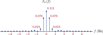
The total power in the signal x (t) can be easily determined using the left side of Eqn. (4.307), i.e.,
The de power in the signal x (t) is
The power in the fundamental frequeney is
Power values for the seeond and third harmonies ean be found similarly as
and
The third harmonie is at frequeney f = 1 Hz. Thus, the power above 1 Hz ean be determined by subtraeting the power values for the de and the first three harmonies from the total, i.e.,
Example 4.39: Power spectral density of a sinusoidal signal
Find the power speetral density of the signal .
Solution: Using Euler’s formula, the signal in question ean be written as
from an inspeetion of whieh we eonelude that the only signifieant eoeffieients in the EFS representation of the signal are
with all other eoeffieients equal to zero. The fundamental frequeney is f0 = 100 Hz. Using Eqn. (4.315), the power speetral density is
whieh is shown in Fig. 4.83
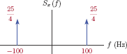
Example 4.40: Energy spectral density of a rectangular pulse
Determine the energy spectral density of the rectangular pulse
Solution: It was determined in Example 4.12 that
Thus the Fourier transform of the pulse given above is
and the energy spectral density is
This result is shown in Fig. 4.84.

Example 4.41: Energy spectral density of the sinc function
Determine the energy spectral density of the signal
Afterwards, compute (a) the total energy in the sinc pulse, and (b) the energy in the sinc pulse at frequencies up to 3 Hz.
Solution: The spectrum of a sinc pulse is a rectangle. Through the use of the duality property of the Fourier transform, X (f) is found to be
The energy spectral density is
which is shown in Fig. 4.85. The total energy in the signal x (t) is

The energy at frequencies up to 3 Hz is found by integrating Gx (f) in the interval −3 Hz < f < 3 Hz:
Fig. 4.86 illustrates the use of Gx (f) for computing the signal energy.

Use of energy spectral density for computing signal energy: (a) total area under Gx (f) corresponding to total energy of the signal, (b) partial area under Gx (f) corresponding to signal energy in frequencies up to 3 Hz.
4.4.3 Autocorrelation
The energy spectral density Gx (f) or the power spectral Sx (f) density for a signal can be computed through direct application of the corresponding equations derived in Section 4.4.2; namely Eqn. (4.321) for an energy signal, and either Eqn. (4.315) or Eqn. (4.326) for a power signal, depending on its type. In some circumstances it is also possible to compute both from the knowledge of the autocorrelation function which will be defined in this section. Let x (t) be a real-valued signal.
For an energy signal x (t) the autocorrelation function is defined as
For a periodic power signal with period T0, the corresponding definition of the autocorrelation function is
The triangle brackets indicate time average. The autocorrelation function for a periodic signal is also periodic as signified by the tilde (~) character used over the symbol τxx in Eqn. (4.328). Finally, for a non-periodic power signal, the corresponding definition is
Even though we refer to rxx(τ) as a function, we will often treat it as if it is a continuous-time signal, albeit one that uses a different independent variable, τ, than the signal x (t) for which it is computed. The variable τ simply corresponds to the time shift between the two copies of x (t) used in the definitions of Eqns. (4.327) through (4.329).
It can be shown that, for an energy signal, the energy spectral density is the Fourier transform of the autocorrelation function, that is,
Proof: Let us begin by applying the Fourier transform definition to the autocorrelation function rxx (τ) treated as a continuous-time signal:
The two integrals in Eqn. (4.331) can be rearranged to yield
Realizing that the inner integral in Eqn. (4.333) is equal to
Eqn. (4.333) becomes
and we obtain
which completes the proof.
The definition of the autocorrelation function for a periodic signal can be used in a similar manner in determining the power spectral density of the signal.
Let the signal and the autocorrelation function , both periodic with period T0, have the EFS representations given by
and
respectively. It can be shown that the EFS coefficients {ck} and {dk} are related by
and the power spectral density is the Fourier transform of the autocorrelation function, that is,
Proof: Using the EFS analysis equation given by Eqn. (4.72) with the definition of the autocorrelation function in Eqn. (4.328) leads to
Rearranging the order of the two integrals Eqn. (4.342) can be written as
Using the time shifting property of the EFS given by Eqn. (4.113) the expression in square brackets in Eqn. (4.343) is
Substituting Eqn. (4.344) into Eqn. (4.343) yields
Recognizing that
since is real, we conclude
Using the technique developed in Section 4.3.6 the Fourier transform of is
Using Eqn. (4.345) in Eqn. (4.347) results in
which is identical to the expression given by Eqn. (4.315) for the power spectral density of a periodic signal.
A relationship similar to the one expressed by Eqn. (4.341) applies to random processes that are wide-sense stationary, and is known as the Wiener-Khinchin theorem. It is one of the fundamental theorems of random signal processing.
Example 4.42: Power spectral density of a sinusoidal signal revisited
Find the autocorrelation function for the signal
Afterwards determine the power spectral density from the autocorrelation function.
Solution: Using Eqn. (4.328) with T0 = 0.01 s we have
Using the appropriate trigonometric identity 7 the integral is evaluated as
Power spectral density is the Fourier transform of the autocorrelation function:
which is in agreement with the earlier result found in Example 4.39.
Properties of the autocorrelation function
The autocorrelation function as defined by Eqns. (4.327), (4.328) and (4.329) has a number of important properties that will be listed here:
rxx (0) ≥ |rxx(τ)| for all τ.
To see why this is the case, we will consider the non-negative function [x (t) ∓ x (t + τ)]2. The time average of this function must also be non-negative, so we can write
or equivalently
which implies that
which is the same as property 1.
- rxx (-τ) = rxx (τ) for all τ, that is, the autocorrelation function has even symmetry. Recall that the autocorrelation function is the inverse Fourier transform of the power spectral density, i.e., . We know from the symmetry properties of the Fourier transform that, since Sx (f) is purely real, rxx (τ) mustbean even function of τ.
If the signal x (t) is periodic with period T, then its autocorrelation function is also periodic with the same period, that is, if for all integers k, then for all integers k.
This property easily follows from the time-average based definition of the autocorrelation function given by Eqn. (4.328). The time average of a periodic signal is also periodic with the same period.
4.5 System Function Concept
In time-domain analysis of systems in Chapter 2 we have relied on two distinct description forms for CTLTI systems:
- A linear constant-coefficient differential equation that describes the relationship between the input and the output signals
- An impulse response which can be used with the convolution operation for determining the response of the system to an arbitrary input signal
In this section, the concept of system function will be introduced as the third method for describing the characteristics of a system.
The system function is simply the Fourier transform of the impulse response:
Recall that the impulse response is only meaningful for a system that is both linear and time-invariant, since the convolution operator could not be used otherwise. Consequently, the system function concept is valid for linear and time-invariant systems only.
In general, H (ω) is a complex function of ω, and can be written in polar form as
Example 4.43: System function for the simple RC circuit
The impulse response of the RC circuit shown in Fig. 4.87 was found in Example 2.18 to be

Determine the system function.
Solution: Taking the Fourier transform of the impulse response we obtain
To simplify notation we will define ωc = 1/RC and write the system function as
The magnitude and the phase of the system function are
and
respectively. The results found in Eqns. (4.352) and (4.352) are shown in Fig. 4.88.
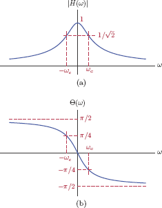
The value of the system function at the frequency ωC is H (ωc) = 1/(1 + j), and the corresponding magnitude is . Thus, ωC represents the frequency at which the magnitude of the system function is 3 decibels below its peak value at ω = 0, that is,
The frequency ωc is often referred to as the 3-dB cutoff frequency of the system.
Software resources:
ex_4_43.m
Interactive Demo: sf_demol.m
The demo program "sf _demol .m" illustrates the system function concept for the simple RC circuit of Example 4.43. The demo program allows circuit parameters R and C to be varied using slider controls, and displays the effect of parameter changes on the magnitude and the phase of the system function.
- Observe how the two variable parameters are related to the 3-dB cutoff frequency fc and consequently the bandwidth of the system function. One particular bandwidth measure called the 3-dB bandwidth is defined as the frequency range in which the magnitude of the system function remains within 3-dB of its peak value, or greater than in this case.
- Pay attention to the value of the phase of the system function at the frequency f = fc.
Software resources:
sf demo1.m
See MATLAB Exercise 4.5. |
Obtaining the system function from the differential equation
Sometimes we need to find the system function for a CTLTI system described by means of a differential equation. Two properties of the Fourier transform will be useful for this purpose; the convolution property and the time differentiation property.
- Since the output signal is computed as the convolution of the impulse response and the input signal, that is, , the corresponding relationship in the frequency domain is . Consequently, the system function is equal to the ratio of the output transform to the input transform:
Using the time differentiation property the transforms of the individual terms in the differential equation are
The system function is obtained from the differential equation by first transforming both sides of the differential equation through the use of Eqns. (4.353) and (4.354), and then using Eqn. (4.352).
Example 4.44: Finding the system function from the differential equation
Determine the system function for a CTLTI system described by the differential equation
Solution: Taking the Fourier transform of both sides of the differential equation we obtain
or
The system function is
4.6 CTLTI Systems with Periodic Input Signals
In earlier sections of this chapter we have developed methods for representing periodic signals as linear combinations of sinusoidal or complex exponential basis functions. Using the TFS representation we have
Alternatively, using the EFS representation
If a periodic signal is used as input to a CTLTI system, the superposition property can be utilized for finding the output signal. The response of the CTLTI system to the periodic signal can be determined as a linear combination of its responses to the individual basis functions in the TFS or EFS representation. We will analyze this concept in two steps; first for a complex exponential input signal, and then for a sinusoidal signal.
4.6.1 Response of a CTLTI system to complex exponential signal
Consider a CTLTI system with impulse response h (t), driven by an input signal in the form of a complex exponential function of time
The response y (t) of the system can be found through the use of the convolution relationship as we have derived in Section 2.7.2 of Chapter 2.
Using the signal given by Eqn. (4.355) in Eqn. (4.356) we get
or, equivalently
The integral in Eqn. (4.358) should be recognized as the system function evaluated at the specific radian frequency ω = ω0. Therefore
The development in Eqns. (4.357) through (4.359) is based on the inherent assumption that the Fourier transform of h (t) exists. This in turn requires the corresponding CTLTI system to be stable. Any natural response the system may have exhibited at one point would have disappeared a long time ago. Consequently, the response found in Eqn. (4.359) is the steady-state response of the system.
For a CTLTI system driven by a complex exponential input signal, we have the following important relationship:
- The response of a CTLTI system to a complex exponential input signal is a complex exponential output signal with the same frequency ω0.
- The effect of the system on the complex exponential input signal is to
- (a) Scale its amplitude by an amount equal to the magnitude of the system function at ω = ω0
- (b) Shift its phase by an amount equal to the phase of the system function at ω = ω0
4.6.2 Response of a CTLTI system to sinusoidal signal
Let the input signal to the CTLTI system under consideration be a sinusoidal signal in the form
The response of the system in this case will be determined by making use of the results of the previous section.
We will use Euler’s formula to write the input signal using two complex exponential functions as
This representation of allows the results of the previous section to be used. The output signal can be written using superposition:
If the impulse response h (t) is real-valued, the result in Eqn. (4.363) can be further simplified. Recall from Section 4.3.5 that, for real-valued h (t), the transform H (w) is conjugate symmetric, resulting in
Using these relationships, Eqn. (4.363) becomes
For a CTLTI system driven by a cosine input signal, we have the following important relationship:
Response to cosine input:
- When a CTLTI system is driven by single-tone input signal at frequency ω0, its output signal is also a single-tone signal at the same frequency.
- The effect of the system on the input signal is to
- (a) Scale its amplitude by an amount equal to the magnitude of the system function at ω = ω0
- (b) Shift its phase by an amount equal to the phase of the system function at ω = ω0
Example 4.45: Steady-state response of RC circuit for single-tone input
Consider the RC circuit of Example 4.43. Let the component values be chosen to yield a 3-dB cutoff frequency of ω c = 160 π rad/s, or equivalently fc = 80 Hz. Let the input signal be in the form
Compute the steady-state output signal for the cases f1 = 20 Hz, f2 = 100 Hz, f3 = 200 Hz, and f4 = 500 Hz.
Solution: For the system under consideration the system function is
The magnitude and the phase of the system function were determined in Example 4.43 Eqns. (4.352) and (4.352). Using f instead of ω we have
as shown in Fig. 4.89. For the input frequency of f1 = 20 Hz, the magnitude and the phase of the system function are

and
The impact of the system on the 20 Hz input signal is amplitude scaling by a factor of 0.9701 and phase shift by −0.245 radians. The corresponding steady-state output signal is
The phase shift of −0.245 radians translates to a time-delay of about td = 1.9 ms. The steady-state output signal y1 (t) is shown in Fig. 4.90 along with the input signal for comparison.

Calculations in Eqns. (4.368) through 4.370) can easily be repeated for the other three frequency choices, but will be skipped here to save space. The results are summarized in Table 4.6 for all four frequencies. The frequency-discriminating nature of the system is evident.
Amplitude scaling, phase offset and time delay values for Example 4.45.
f (Hz) |
|H (f)| |
Θ (f) (rad) |
td (ms) |
|---|---|---|---|
20 |
0.9701 |
−0.2450 |
1.95 |
100 |
0.6247 |
−0.8961 |
1.43 |
200 |
0.3714 |
−1.1903 |
0.94 |
500 |
0.1580 |
−1.4121 |
0.45 |
Input-output signal pairs for f2 = 100 Hz, f3 = 200 Hz, and f4 = 500 Hz are shown in Fig. 4.91.
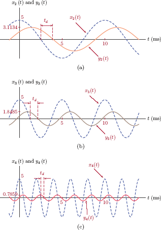
The input-output signal pairs for Example 4.45: (a) f2 = 100 Hz, (b) f3 = 200 Hz, and (c) f4 = 500 Hz.
Software resources:
ex_4_45a.m
ex_4_45b.m
ex_4_45c.m
Interactive Demo: sf_demo2.m
The demo program “sf_demo2.m” parallels the development of Example 4.45. Magnitude, phase and time-delay characteristics of the system function under consideration are shown. The first slider control allows the value of fc to be adjusted. With the choice of fc = 80 Hz the transfer function of Example 4.45 is obtained. The second slider control specifies the frequency of the input signal which is marked on the magnitude, phase and time-delay graphs. At the bottom of the screen, input and output signals are shown along with delay markers that illustrate the delay caused by the system.
- Verify the numerical results of Example 4.45 by using fc = 80 Hz, and setting the signal frequency equal to f1 = 20 Hz, f2 = 100 Hz, f3 = 200 Hz, and f4 = 500 Hz. Compare input and output signals to those in Figs. 4.90 and 4.91.
- With the signal frequency fixed at f2 = 100 Hz, change the 3-dB bandwidth of the system and observe its effect on the output signal in terms of peak amplitude and time delay.
Software resources:
sf_demo2.m
4.6.3 Response of a CTLTI system to periodic input signal
Using the development in the previous sections, we are now ready to consider the use of a general periodic signal as input to a CTLTI system. Let be a signal that satisfies the existence conditions for the Fourier series. Using the EFS representation of the signal, the response of the system is
Let us use the linearity of the system to write the response as
The response of the system to an exponential basis function at frequency ω = kωo is given by
Using Eqn. (4.373) in Eqn. (4.372), the response of the system to is found as
Two important observations should be made based on Eqn. (4.374):
- For a CTLTI system driven by a periodic input signal, the output signal is also periodic with the same period.
- If the EFS coefficients of the input signal are {ck; k= 1, ..., ∞} then the EFS coefficients of the output signal are {ck H (kω0); k = 1, ..., ∞}.
Example 4.46: RC circuit with pulse-train input
Consider again the RC circuit used in Example 4.45 with system function given by Eqn. (4.368). Let the input signal be a pulse train with period T0 = 50 ms and duty cycle d = 0.2 as shown in Fig. 4.92. Determine the output signal in steady state.
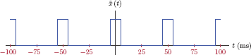
Solution: The EFS coefficients were determined in Example 4.7 for the type of periodic pulse train shown in Fig. 4.92. Using the specified duty cycle the coefficients are
The fundamental frequency is f0 = 1/T0 = 20 Hz, and the EFS representation of the signal is
Let {dk ; k = −∞,..., ∞] be the EFS coefficients of the output signal . Using Eqn. (4.374) we have
The EFS representation of the output signal is
Using the expressions for the magnitude and the phase of the system function, Eqn. (4.377) can be written as
and
The relationship between the system function H (f) and the line spectra ck and dk is illustrated in Fig. 4.93. An approximation to the output signal using terms up to the 75-th harmonic is shown in Fig. 4.94.

System function and line spectra for Example 4.46: (a) the magnitude of the system function, (b) the phase of the system function, (c) the magnitude of the input spectrum, (d) the phase of the input spectrum, (e) the magnitude of the output spectrum, (f) the phase of the output spectrum.

The response of the system in Example 4.5 to pulse train with period T0 = 20 ms and duty cycle d = 0.2.
Software resources:
ex_4_46a.m
ex_4_46b.m
Interactive Demo: sf_demo3.m
The demo program “sf_demo3.m” is based on Example 4.46, and illustrates the use of the system function with the exponential Fourier series coefficients of a periodic signal. The system under consideration is the RC circuit that we have used extensively in this chapter. The input signal is a periodic pulse train the period and the duty cycle of which may be adjusted using the slider controls. Continuing with the notation established in Example 4.46, we will let ck and dk represent the line spectra of the input and the output signals respectively. In the demo program, only the magnitude spectra |ck| and |dk| are shown due to screen size constraints.
- Observe the effect of the period T0 on the placement of spectral lines in the frequency spectra of input and output signals. The line spectra |ck| and |dk| are displayed not in terms of the index k but rather in terms of the actual frequencies kfo.
- Observe how the system function H (f) effects the line spectrum for the output signal. Compare the line spectra for the input and the output signals. The more different the two line spectra are, the more different the two time domain signals and will be.
Software resources:
sf_demo3.m
4.7 CTLTI Systems with Non-Periodic Input Signals
Let us consider the case of using a non-periodic signal x (t) as input to a CTLTI system. We have established in Section 2.7.2 of Chapter 2 that the output of a CTLTI system is equal to the convolution of the input signal with the impulse response, that is
Let us assume that
- The system is stable ensuring that H (ω) converges
- The input signal has a Fourier transform
We have seen in Section 4.3.5 of this chapter that the Fourier transform of the convolution of two signals is equal to the product of individual transforms:
The output transform is the product of the input transform and the system function.
Writing each transform involved in Eqn. (4.382) in polar form using its magnitude and phase we obtain the corresponding relationships:
- The magnitude of the output spectrum is equal to the product of the magnitudes of the input spectrum and the system function.
- The phase of the output spectrum is found by adding the phase characteristics of the input spectrum and the system function.
Example 4.47: Pulse response of RC circuit revisited
Consider again the RC circuit used Example 4.43. Let fc = 1/RC = 80 Hz. Determine the Fourier transform of the response of the system to the unit-pulse input signal x (t) = ∏ (t).
Solution: In Example 2.21 of Chapter 2 the output signal y (t) was found through the use of convolution operation. In this example we will approach the same problem from a system function perspective. The system function of the RC circuit under consideration was found in Example 4.43 to be
The transform of the output signal is
Using fc = 80 Hz, the transform of the output signal is
Magnitude and phase of the transform Y (ω) can be found using Eqns. (4.383) and (4.384). The magnitude is
and the phase is
as illustrated in Fig. 4.95. With a bit of work it can be shown that Y (f) found above is indeed the Fourier transform of the signal y (t) found in Example 2.21 using the convolution integral.
Software resources:
ex_4_47.m
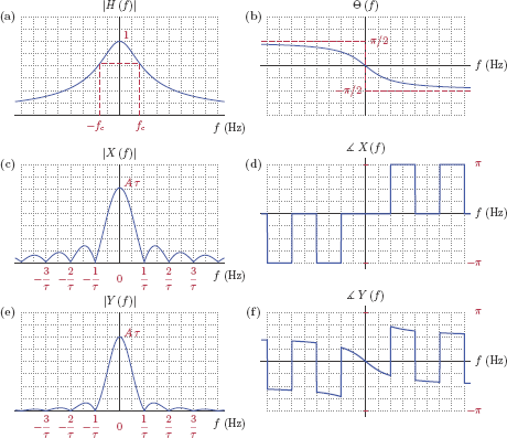
Determining the Fourier transform of the output signal of a linear system: (a) the magnitude of the system function, (b) the phase of the system function, (c) the magnitude of the input spectrum, (d) the phase of the input spectrum, (e) the magnitude of the output spectrum, (f) the phase of the output spectrum.
Interactive Demo: sf_demo4.m
The demo program “sf_demo4.m” is based on Example 4.47, and illustrates the use of the system function in conjunction with the Fourier transform of a pulse. The transform of the output signal is the product of the system function with the transform of the input signal as we have established in Eqns. (4.385) through (4.387). The input signal x (t) is a single pulse with unit amplitude and width equal to τ, and it is centered around t = 0. The user interface of the demo program displays magnitudes of the three transforms involved, namely X (f), H (f) and Y (f). Time domain representations of the input and the output signals are also shown. Phase characteristics are not displayed in the demo due to screen space constraints. System parameter fc and input signal parameter τ may be varied using slider controls, and the effect of these variations may be observed on magnitude spectra as well as the output signal.
- Observe how the changes to the system function affect the magnitude spectrum of the output signal.
- Specifically, how does the bandwidth of the system impact the shape of the output pulse. How does the bandwidth of the system function relate to the level of similarity between the input and the output signals?
- Vary the duration τ of the input pulse. How does the pulse duration relate to the level of similarity between the input and the output signals?
Software resources:
sf_demo4.m
4.8 Further Reading
[1] R.J. Beerends. Fourier and Laplace Transforms. Cambridge University Press, 2003.
[2] R.N. Bracewell. The Fourier Transform and Its Applications. Electrical Engineering Series. McGraw-Hill, 2000.
[3] E.A. Gonzalez-Velasco. Fourier Analysis and Boundary Value Problems. Elsevier Science, 1996.
[4] R. Haberman. Applied Partial Differential Equations: With Fourier Series and Boundary Value Problems. Pearson Education, 2012.
[5] K.B. Howell. Principles of Fourier Analysis. Studies in Advanced Mathematics. Taylor & Francis, 2010.
MATLAB Exercises
MATLAB Exercise 4.1: Computing finite-harmonic approximation to pulse train
Develop a MATLAB script to compute and graph the finite-harmonic approximation to the periodic pulse train of Example 4.1 for m = 4.
Solution: Consider the listing given below:
1 % Script matex_4_1.m
2 %
3 m = 4; % Number of harmonics to be used.
4 t = [-7:0.01:7]; % Create a vector of time instants.
5 f0 = 1/3; % Fundamental frequency is f0 = 1/3 Hz.
6 omegaO = 2*pi*f0;
7 x = 1/3; % Recall that a0=1/3.
8 % We will start by setting x(t) = a0.
9 % Start the loop to compute the contribution of each harmonic.
10 for k = 1:m,
11 ak = 1/(pi*k)* sin (k*omega0);
12 bk = 1/(pi*k)*(1 - cos (k* omega0));
13 x = x+ak*cos(k*omega0*t)+bk*sin(k*omega0*t);
14 end ;
15 % Graph the resulting approximation to x(t).
16 clf ;
17 plot(t,x); grid;
18 title('Approximation using m=4'),
19 xlabel ('Time (sec)'),
20 ylabel ('Amplitude'),
The main part of the code is the loop construct between lines 10 and 14. Before entering the loop, the vector “x” holds a zero-order approximation to the signal, that is, = ω0 = 1/3. After the first pass through the loop, the vector “x” holds samples of the signal
After the second pass through the loop, the vector “x” now holds
and so on. The graph produced by this listing is shown in Fig. 4.96.

Software resources:
matex 4 1.m
MATLAB Exercise 4.2: Computing multiple approximations to pulse train
MATLAB listing given below computes all approximations to the periodic pulse train of Example 4.1 for m = 1,..., 5. The approximations , , , , are graphed on the same coordinate system for comparison. The approximation is not graphed since a3 = b3 = 0 based on Table 4.1, and therefore .
1 % Script : matex_4_2.m
2 %
3 m = 5; % Maximum number of harmonics to be used.
4 t = [-3:0.005:3]; % Create a vector of time instants.
5 f0 = 1/3; % Fundamental frequency is f0 =1/3 Hz.
6 omega0 = 2*pi*f0;
7 x = 1/3* ones(size(t)); % Recall that a0=1/3.
8 % We will start by setting x(t) = a0.
9 xmat = x; % Row vector containing dc value of 1/3.
10 % Start the loop to compute the contribution of each harmonic.
11 for k = 1:m,
12 ak = 1/(pi*k) *sin (k*omega0);
13 bk = 1/(pi*k)*(1 - cos (k* omega0));
14 x = x+ak*cos(k*omega0*t)+bk*sin(k*omega0*t);
15 xmat = [xmat ;x] ; % Append another row to matrix 'xmat'.
16 end;
17 % Graph the results.
18 clf ;
19 plot (t,xmat(2,:),'b--',t,xmat(3,:),'g-',t,xmat(5,:),'r-',...
20 t, xmat (6 ,:) , 'm-') ; grid;21 title('Approximation to x(t) using m=1,...,5'),
22 xlabel ('Time (sec)'),
23 ylabel ('Amplitude'),
24 legend ('x^{(1)}(t) ','x^{(2)}(t)','x^{(4)}(t)','x^{(5)}(t)'),
On line 9 the matrix “xmat” is initialized as a row vector holding the constant (zero-order) approximation to . The loop construct between lines 11 and 16 is a slightly modified version of the corresponding construct in MATLAB Exercise 4.1. At each pass through the loop a new row is added to the matrix “xmat” as the next approximation to the periodic signal. When the script is finished, the rows of the matrix “xmat” correspond to finite-harmonic approximations as follows:
The graph produced by this script is shown in Fig. 4.97.

Software resources:
matex 4 2.m
MATLAB Exercise 4.3: Graphing the line spectrum in Example 4.5
The line spectrum found in Example 4.5 can be graphed in MATLAB using a direct implementation of the general expression found in Eqn. (4.73) for the EFS coefficients. The code given below computes and graphs the spectrum in the index range −25 ≤ k ≤25.
1 % Script : matex_4_3a.m
2 %
3 k = [-25:25]; % Create a vector of index values.
4 k = k+eps; % Avoid division by zero.
5 ck = sin(pi*k/3)./(pi*k); % Compute the EFS coefficients.
6 % Graph the line spectrum.
7 clf;
8 stem(k,ck);
9 axis ([-25.5 ,25.5 , -0.1 ,0.4]);
10 xlabel ('Index k'),
11 ylabel ('Coefficient '),
The resulting line spectrum graph is shown in Fig. 4.98.

Recall that the general expression for ck as given by Eqn. (4.73) produced an indefinite value at k = 0 necessitating the use of L'Hospital's rule. Without any precautions, line 3 of the code given above would produce a division by zero error for k = 0. To avoid this, we add a very small positive value to all indices. This is done in line 2 of the code with the statement
4 k = k + eps;
MATLAB has a built-in variable eps for this purpose. It is the smallest positive floatingpoint number MATLAB can represent, and therefore its effect on the end result should be negligible. An alternative and perhaps tidier method of avoiding the division-by-zero error is to use the sinc function defined as
which allows the result of Eqn. (4.73) to be written in the form
MATLAB function sinc (..) computes the value at k = 0 correctly without requiring any special precautions on our part. A modified script file that uses the function sinc(..) and produces the same graph is given below:
1 % Script: matex_4_3b.m
2 %
3 k = [-25:25]; % Create a vector of index values.
4 ck = 1/3*sinc(k/3); % Compute the EFS coefficients.
5 % Graph the line spectrum.
6 clf;
7 stem(k,ck);
8 axis([-25.5,25.5,-0.1,0.4]);
9 xlabel('Index k'),
10 ylabel('Coefficient'),
If the line spectrum is desired in polar form with magnitude and phase, lines 7 through 10 of the script listed above may be replaced with the following:
8 subplot (2, 1, 1);
9 stem(k,abs(ck));
10 axis ([-25.5, 25.5, -0.1, 0.4]);
11 xlabel ('Index'),
12 ylabel ('Magnitude'),
13 subplot (2,1,2);
14 stem(k, angle (ck));
15 axis ([-25.5 ,25.5 ,-4 ,4]) ;
16 xlabel ('Index'),
17 ylabel ('Phase (rad)'),
Magnitude and phase of the EFS coefficients are graphed through the use of MATLAB functions abs(..) and angie(..) respectively. The resulting graph is shown in Fig. 4.99.

Software resources:
matex 4 3a.m
matex 4 3b.m
matex 4 3c.m
MATLAB Exercise 4.4: Line spectrum for Example 4.6
MATLAB listing given below can be used for computing and displaying the EFS coefficients for the signal of Example 4.6 for k = −25,..., 25. Eqns. (4.74) and (4.75) are graphed as functions of the integer index k.
1 % Script: matex_4_4a.m
2 %
3 k = [-25:25]; % Create a vector of index values.
4 k = k+eps; % Avoid division by zero.
5 cReal = 1./(2*pi*k).*sin(2*pi*k/3);
6 cImag = 1./(2*pi*k).*(cos(2*pi*k/3)-1);
7 cMag = abs (cReal+j*cImag);
8 cPhs = angle (cReal + j*cImag);
9 % Graph the line spectrum.
10 clf ;
11 subplot (2,1,1);
12 stem(k, cMag) ;
13 axis ([-25.5, 25.5 , -0.1, 0.4]);
14 title ('| c_{k} | '),
15 xlabel('Index k'),
16 ylabel (' Magnitude '),
17 subplot (2,1,2);
18 stem(k, cPhs) ;
19 axis ([-25.5 ,25.5 ,-4 ,4]);
20 title ('angle c_{k}'),
21 xlabel('Index k'),
22 ylabel ('Phase (rad) '),
A finite-harmonic approximation to the signal can be computed and graphed using the script below:
1 % Script: matex_4_4b.m
2 %
3 f0 = 1/3; % Fundamental frequency.
4 omegaO = 2*pi*f0;
5 t = [-3:0.01:6]; % Create a vector of time instants.
6 x = zeros(size(t)); % Start with a vector of all zeros.
7 for k = -25:25
8 k = k+eps; % Avoid division by zero.
9 cReal = 1/(2*pi*k)*sin(k*omega0);
10 cImag = 1/(2*pi*k)*(cos(k*omega0)-1);
11 x = x+(cReal+j*cImag)*exp(j*k*omega0*t);
12 end ;
13 % Graph the signal.
14 clf;
15 plot(t, real (x)) ; grid;
16 title('Approximation to x(t)'),
17 xlabel ('Time (sec)'),
18 ylabel ('Amplitude'),
On line 15 of the code we use the real(..) function on the vector “x” to remove any residual imaginary part that may be introduced as a result of round-off error.
Software resources:
matex_4_4a.m
matex_4_4b.m
MATLAB Exercise 4.5: Graphing system function for RC circuit
MATLAB code listing given below can be used for computing and graphing the system function found in Eqn. (4.351) of Example 4.43 in the frequency range −1 Hz ≤ f ≤1 Hz.
1 % File: matex_4_S.m
2 %
3 R = 1 e6;
4 C = 1 e-6;
5 fc = 1/(2*pi*R*C); % The critical frequency
6 f = [-500:500]/500; % Vector of frequency values
7 Hf = 1./(1+j*f/fc); % Evaluate system function
8 % Graph the magnitude and the phase
9 clf;
10 subplot (2,1,1);
11 plot(f, abs (Hf)); grid;
12 axis ([-1 ,1 ,-0.2 ,1.2]) ;
13 ylabel (' Magnitude ') ;
14 xlabel ('Frequency (Hz)'),
15 subplot (2, 1, 2);
16 plot (f, angle(Hf)); grid;
17 ylabel ('Phase (rad)'),
18 xlabel(' Frequency (Hz)'),
Note that line 7 of the code is a direct implementation of Eqn. (4.351) with f and fc in Hz used instead of radian frequencies ω and ωc.
Software resources:
matex_4_5.m
Problems
4.1. Consider the periodic square-wave signal shown in Fig. 4.1 on page 267.
Set up the cost function for approximating this signal using three terms in the form
Show that the optimum values of the coefficients are
4.2. Consider the pulse train shown in Fig. P.4.2.
- Determine the fundamental period T0 and the fundamental frequency ω0 for the signal.
Using the technique described in Section 4.2 find an approximation to in the form
Determine the optimum coefficients a0, a1 and b1.
4.3. Consider again the pulse train shown in Fig. P.4.2. Using the technique described in Section 4.2 find an approximation to in the form
4.4. Consider again the periodic square-wave signal shown in Fig. 4.1. The approximation using M trigonometric functions would be in the form
Show that the approximation error is equal to ±A at discontinuities of the signal independent of the number of terms M, that is,
Hint: It should not be necessary to determine the optimum coefficient values b1, b2,..., bM for this problem.
4.5. Consider the pulse train shown in Fig. P.4.5.
- Determine the fundamental period T0 and the fundamental frequency ω0 for the signal.
Using the approach followed in Section 4.2 determine the coefficients of the approximation
to the signal that results in the minimum mean-squared error.
4.6. Refer to the TFS representation of a periodic signal given by Eqn. (4.26). Using the orthogonality properties of the basis functions show that the coefficients of the sine terms are computed as
where T0 is the fundamental period, ω0 = 2π/T0 is the fundamental frequency in rad/s and t0 is an arbitrary time instant.
4.7. Determine the TFS coefficients for the periodic signal shown in Fig. P.4.7.
4.8. Determine the TFS coefficients for the periodic signal shown in Fig. P. 4.8. One period of the signal is for 0 ≤ t ≤ 1 s.
4.9. Consider the periodic signal shown in Fig. P.4.7.
- Determine the EFS coefficients from the TFS coefficients obtained in Problem 4.7.
- Determine the EFS coefficients by direct application of the analysis equation given by Eqn. (4.72).
- Sketch the line spectrum (magnitude and phase).
4.10. Consider the periodic signal shown in Fig. P.4.8.
- Determine the EFS coefficients from the TFS coefficients obtained in Problem 4.8.
- Determine the EFS coefficients by direct application of the analysis equation given by Eqn. (4.72).
- Sketch the line spectrum (magnitude and phase).
4.11. Consider the periodic sawtooth signal shown in Fig. P.4.11.
- Determine EFS coefficients of this signal using the analysis equation in Eqn. (4.72).
- Sketch the line spectrum in terms of magnitude and phase.
- Determine the TFS coefficients of from the EFS coefficients using the conversion formulas given by Eqns. (4.58) and (4.59).
4.12. Let the periodic signal have the EFS coefficients ck. A new periodic signal is defined as a time reversed version of , that is,
- If has the EFS coefficients dk, find the relationship between the two sets of coefficients ck and dk.
- Consider the signal shown in Fig. 4.17 on page 290. Its EFS coefficients of were determined in Example 4.8 and given by Eqns. (4.81) and (4.82). Obtain the EFS coefficients of shown in Fig. P.4.11 from the EFS coefficients of using the results of part (a).
4.13. The signal shown in Fig. 4.17 and the signal shown in Fig. P4.11 add up to a constant:
Explain how this property can be used for finding the EFS coefficients of from the EFS coefficients of that were determined in Example 4.8 and given by Eqns. (4.81) and (4.82).
4.14. Determine the EFS coefficients of the full-wave rectified signal shown in Fig. P.4.14.
4.15. Prove the time shifting property of the exponential Fourier series given by Eqn. (4.113). Specifically show that, if the periodic signal has the EFS coefficients ck, then the signal has the coefficients
4.16. Refer to the half-wave rectified sinusoid shown in Fig. 4.21 on page 293. Its EFS coefficients were determined in Example 4.10. Explain how the EFS coefficients of the full-wave rectified sinusoid in Fig. P.4.14 could be obtained from the results of Example 4.10 through the use of the time shifting property.
4.17. Refer to the half-wave rectified sinusoid shown in Fig. 4.21. Its EFS coefficients were determined in Example 4.10. Using the conversion formulas given by Eqns. (4.92) and (4.93) find the compact Fourier series (CFS) representation of the signal.
4.18. Find the Fourier transform of each of the pulse signals given below:
- x (t) = 3 ∏ (t)
- x (t) = 3 ∏ (t − 0.5)
4.19. Starting with the Fourier transform integral given by Eqn. (4.129) find the Fourier transform of the signal
shown in Fig. P.4.19.
4.20. Starting with the Fourier transform integral given by Eqn. (4.129) find the Fourier transform of the signal
shown in Fig. P.4.20. Assume a ≥ 0.
4.21. Refer to the signal shown in Fig. P.4.19. Find its Fourier transform by starting with the transform of the unit pulse and using linearity and time shifting properties.
4.22. Refer to the signal shown in Fig. P.4.20. Find its Fourier transform by starting with the transform of the right-sided exponential signal and using linearity and time scaling properties.
4.23. The Fourier transform of the triangular pulse with peak amplitude A and two corners at ±τ was found in Example 4.17 as
Using this result along with linearity and time shifting properties of the Fourier transform, find the transform of the signal shown in Fig. P.4.23.
-
was obtained in Example 4.16. Using this pair along with the duality property, find the Fourier transform of the signal
4.25. Prove that, for a real-valued signal with odd symmetry, the Fourier transform is purely imaginary.
Hint: Start with the conditions x* (t) = x (t) and x (−t) = −x (t). Show that Re {X (ω)} = 0.
4.27. Compute and sketch the Fourier transforms of the modulated pulse signals given below:
- x (t) = cos (10πt) ∏ (t)
- x (t) = cos (10πt) ∏ (2t)
- x (t) = cos (10πt) ∏ (4t)
-
- Starting with the inverse Fourier transform integral given by Eqn. (4.129) prove the second form of the differentiation-in-time property stated in Eqn. (4.249) for n = 1.
- Show that, if Eqn. (4.249) holds true for n = k where k is any positive integer, then it must also hold true for n = k + 1.
-
- Starting with the Fourier transform integral given by Eqn. (4.130) prove the second form of the differentiation-in-frequency property stated in Eqn. (4.265) for n = 1.
- Show that, if Eqn. (4.265) holds true for n = k where k is any positive integer, then it must also hold true for n = k + 1.
4.30. Taking Eqn. (4.249) as a starting point and employing the duality property of the Fourier transform, prove the second form of the differentiation-in-frequency property stated in Eqn. (4.265) for n = 1.
4.31. Using the differentiation-in-time property of the Fourier transform, determine the transform of the signal shown in Fig. P.4.31.
4.32. The Fourier transform of the trapezoidal signal x (t) shown in Fig. 4.70 on page 355 was found in Example 4.32 to be
Find the inverse transform of the spectrum shown in Fig. 4.74 on page 360 by using the result above in conjunction with the duality property.
4.33. Determine the Fourier transform of the signal
- Using the modulation property of the Fourier transform
- Using the multiplication property of the Fourier transform
4.34. Consider the periodic pulse train shown in Fig. P.4.34.
Recall that the EFS coefficients of this signal were found in Example 4.6. Express the Fourier transform of using impulse functions.
4.35. Consider the pulse train with duty cycle d shown in Fig. 4.15 on page 289. Its EFS coefficients were determined in Example 4.7 to be
- Working in the time domain, compute the power of the pulse train as a function of the duty cycle d.
- Sketch the power spectral density based on the EFS coefficients.
- Let d = 0.5. Suppose this signal is processed through a lowpass system that only retains the first m harmonics and eliminates the others. How many harmonics should be retained if we want to preserve at least 90 percent of the signal power?
- How many harmonics should be retained to preserve at least 95 percent of the signal power?
- How many harmonics should be retained to preserve at least 99 percent of the signal power?
4.36. Repeat parts (c)-(e) of Problem 4.35 using d = 0.2. Does it take fewerormore harmonics to preserve the same percentage of power when the duty cycle is reduced?
4.37. Use Parseval's theorem to prove that
4.38. Determine and sketch the power spectral density of the following signals:
- x (t) = 3 cos (20πt)
- x (t) = 2 cos (20πt) + 3 cos (30πt)
- x (t) = 5 cos (200πt) + 5 cos (200πt) cos (30πt)


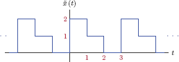
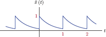

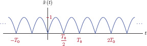


MATLAB Problems
4.39. Refer to Problem 4.1 in which a periodic square-wave signal was approximated using three terms. Let the parameters of the square wave be A = 1 and T0 = 1. Using MATLAB, compute and graph the three-term approximation superimposed with the original signal, that is, graph and on the same coordinate system. Display the signals in the time interval −1.5 < t < 2.5 s.
4.40. Refer to Problem 4.2 in which a periodic pulse train was approximated using using both cosine and sine functions. Using MATLAB, compute and graph the approximation superimposed with the original signal and on the same coordinate system. Show the time interval −1.5 < t < 2.5 s.
4.41. Compute and graph finite-harmonic approximations to the signal shown in Fig. P.4.7 using 3, 4, and 5 harmonics. Also graph the approximation error for each case.
4.42. Compute and graph finite-harmonic approximations to the signal shown in Fig. P.4.8 using 3, 4, and 5 harmonics. Also graph the approximation error for each case.
4.43. Consider the periodic pulse train shown in Fig. 4.15 on page 289. Its EFS coefficients were determined in Example 4.7 and given in Eqn. (4.77). Write a script to compute and graph the EFS line spectrum for duty cycle values d = 0.4, 0.6, 0.8 and 1. Comment on the changes in the spectrum as d is increased.
4.44. Refer to Problem 4.17 in which the CFS representation of a half-wave rectified sinusoidal signal was determined. Write a script to compute and graph finite-harmonic approximations to the signal using m = 2, 4 and 6 harmonics.
4.45. Refer to Problem 4.27. Write a script to compute and graph the transform of the modulated pulse
In your script, define an anonymous function that takes two arguments, namely “f” and “tau”, and returns the spectrum of a pulse with width τ centered around the time origin. Use the result with modulation property of the Fourier transform to compute the transform sought. Use the script to verify the results obtained in Problem 4.27.
4.46. Refer to Problem 4.35.
- Write a script to compute and graph the finite-harmonic approximation to the signal using thefirst m harmonics. Leave m as a parameter that can be adjusted.
- Using the values of m found in parts (c), (d) and (e) of Problem 4.35 compute and graph the finite-harmonic approximations to the signal. Comment on the correlation between the percentage of power preserved and the quality of the finite-harmonic approximation.
MATLAB Projects
4.47. Consider the RC circuit shown in Fig. 4.87 on page 382. Its system function was determined in Example 4.43 to be
Assume that the element values of the circuit are adjusted to obtain a critical frequency of fc = 80 Hz or, equivalently, ωc = 160π rad/s. Let the input signal to this circuit be a periodic pulse train with a period of T0 = 20 milliseconds as shown in Fig. P.4.47.
- Determine the EFS coefficients of the signal as a function of the duty cycle d. Write a script to graph the EFS spectrum of the signal for duty cycle values d = 0.5, 0.3, 0.1.
- Let the pulse width be τ = 10 ms corresponding to a duty cycle of d = 0.5. The signal is used as input to the RC circuit. Write a script to compute the EFS coefficients of the output signal . Also graph the EFS spectrum for the output signal.
- Write a script to construct and graph an approximation to the output signal using the first 30 harmonics in the EFS spectrum.
An alternative to approximating the output of the RC circuit in response to a periodic signal is to determine its response to one isolated period, and then extend the result periodically. Let one period of the input signal be f(t) so that can be expressed as
For the input signal we are considering, f (t) would be
If the response of the RC circuit to one period f (t) is
then the response to the periodic signal is
For d = 0.5 manually determine g(t), the response to a single pulse with τ = 10 ms. Write a script to compute the response using this approach and graph it. In your script use an anonymous function to compute the values of g(t). Approximate the summation for using the terms for r = −20,..., 20. Compare the result obtained through this approach with the one obtained in part (c). What are the differences, and how would you explain them?
- Repeat parts (b) and (d) for duty cycle values d = 0. 3 and 0.1.
4.48. Problem 4.47 should illustrate that the signal at the output of the RC circuit is a distorted version of the input signal. It should also illustrate that the severity of the distortion is dependent on the pulse-width τ and consequently the duty cycle d.
The amount of distortion is also dependent on the shape of the input signal. In digital communication systems that rely on pulses for transmitting information, the fidelity of the output signal is important; the received pulses should be as similar to the transmitted pulses as possible. If alternative pulse shapes can provide better fidelity, they may be preferred over rectangular pulses.
In this problem we will explore the use of an alternative pulse train. Consider the signal shown in Fig. P.4.48 to be used as input in place of the signal of Problem 4.47 with d = 0.5.
A general expression for the EFS coefficients for the signal was obtained in Example 4.10. Repeat parts (a) through (c) of Problem 4.47 using this alternative signal. Comment on the results, especially in comparison to those obtained in Problem 4.47.

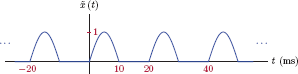
1cos (2a) = 2 cos2 (a) − 1 = 1 − 2 sin2 (a).
4 cos(a + b) = cos(a) cos(b) −sin(a) sin(b).
5 .
6 cos (a + b) = cos (a) cos (b) − sin (a) sin (b).
7 .