
Amplitude Modulation
Chapter Objectives
- Learn the significance of and the need for modulation in analog and digital communication systems.
- Understand amplitude modulation as one method of embedding an information bearing signal into a high frequency sinusoidal carrier.
- Explore time- and frequency-domain characteristics of amplitude modulated signals. Understand variants of amplitude modulation (DSB and SSB).
- Study techniques for obtaining modulated signals as well as extracting information bearing signals from modulated signals.
11.1 Introduction
The main purpose of any communication system is to facilitate the transfer of an information bearing signal from one point in space to another, with an acceptable level of quality.
Consider, for example, two people communicating through their cell phones. The sound of the person who acts as information source is detected by the microphone on his or her phone, converted to an electrical signal for processing within the phone, and eventually converted to an electromagnetic signal which is transmitted from the antenna of the phone. This electromagnetic signal is received by the antennas within the cell phone network, transmitted from cell to cell as needed, possibly travels through various types of connections such fiber optics and satellite links, and finally reaches the antenna of the phone that is designated as its destination. Within the receiving phone, the electromagnetic signal is converted back to an electrical signal, and is eventually converted to sound.
Thus, any communication system has a transmitter and a receiver. The collection of all systems between the transmitter and the receiver is referred to as the communication channel. In general, a channel has two undesirable effects on the signals that are transmitted through it:
As a result, the electrical signal reproduced in the receiving phone and the sound reproduced through its speaker are only approximations of the original signals transmitted. In the design of communication systems we take steps to ensure that the signals at the receiving end are reasonably good representations of the signals transmitted.
In this chapter we will present an introduction to modulation which is one of the steps taken in the design of a communication system to ensure reliable transmission of signals. In doing so, we will utilize the analysis tools and transforms developed in previous chapters for linear systems.
Modulation is the process of embedding an information bearing signal, referred to as the message signal, in another signal known as the carrier. The carrier by itself does not contain any information, yet it may have other features that make it desirable. Some examples of these desirable features are: 1) suitability for transmission through a particular medium, 2) better performance in the presence of noise and interference, 3) suitability to more efficient utilization of resources, and so on.
Fig. 11.1 illustrates the general structure of a very simple analog communication system.

The overall operation of the communication system can be summarized as follows:
The role of the input transducer is to convert the source message from its native format to the form of an electrical signal m (t), referred to as the message signal. Some examples of input transducers are microphone, video camera, pressure gauge, temperature sensor, etc.
The modulator embeds the message signal m (t) into the carrier signal xc (t) to create the modulated carrier x (t) which is then transmitted through the channel.
The output signal of the channel is a distorted version of x (t) which is also contaminated with noise. Insimple terms we have
where Sys {...} represents the effect of the channel on the modulated signal, and w (t) represents the additive channel noise.1
- At the receiver side of the system the demodulator reverses the action of the modulator, and extracts an approximate version of the original message signal m (t) from the received modulated signal y (t). The demodulator may or may not need a local copy of the carrier signal xc (t).
- Finally, the output transducer converts the electrical signal to its native format. Examples of output transducers are speaker, video display, etc.
11.2 The Need for Modulation
We need to address the question of why a modulator and a demodulator are needed in a communication system. Using a modulated carrier for transmitting a message has a number of benefits over transmitting the message signal m (t) directly through the channel without modulation:
Compatibility of the signal with the channel:
Modulation gives us the ability to produce a signal that is compatible with the characteristics of the channel that will transmit it.
Most message signals we encounter in our daily lives involve relatively low frequencies, referred to as the baseband frequencies. For example, voice signals used in telephone communications occupy the frequency range from about 300 Hz to about 3600 Hz. High fidelity music signals are typically in the frequency range from about 20 Hz to about 20 kHz. Similarly, baseband video signals such as those encountered on a TV monitor occupy roughly the frequency range from 0 to about 4.2 MHz. Signals such as these can be transmitted using wire links or optical fiber connections, but they are not suitable for over-the-air transmission due to their large wavelengths. The antennas required for over-the-air transmission of these signals in their original form would have to be unreasonably long. Modulating a high frequency carrier with these message signals makes over-the-air broadcast possible while keeping required antenna lengths at practical levels.
Reduced susceptibility to noise and interference:
Modulation of a carrier with the message signal results in a shift of the range of signal frequencies. This frequency shift can be used in a way that allows us to position the frequency spectrum of the signal where noise and interference conditions are more favorable compared to the conditions at baseband frequencies.
Additionally, some modulation techniques allow performance improvements in terms of noise susceptibility provided that increased bandwidth is available.
Multiplexing:
Modulation allows for more efficient use of available resources by multiplexing different signals in the same medium.
In sinusoidal modulation, the frequency shift that results from modulation can also be used for mixing multiple messages in one medium, with each message signal modulating a carrier at a different frequency. These modulated carrier signals can be combined and transmitted together. They can later be separated from each other provided that the frequency ranges occupied by different carriers do not overlap with each other. This effect is known as frequency division multiplexing (FDM). On radio and television, FDM forms the basis of simultaneous broadcast of multiple stations in the same air space.
In digital pulse modulation, the gaps between the successive pulses of a carrier can be used for accommodating messages from multiple sources, a concept known as time division multiplexing (TDM). Multiple digital information sources can utilize the same channel simultaneously, by taking turns in sending data.
11.3 Types of Modulation
The type of modulation used in a communication system depends on
- The type of carrier used
- The particular parameter of the carrier that is utilized for embedding the message signal into it
We will focus on two commonly used types of carrier signals, namely a sinusoidal carrier and a pulse train. Consider the sinusoidal carrier signal:
The carrier described by Eqn. (11.01) has three parameters, namely the amplitude Ac, the frequency fc and the phase ϕc as shown in Fig. 11.2.
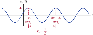
If the values of these three parameters are fixed, then the carrier clearly has no information value since its future behavior is completely predictable. Such a carrier signal is referred to as a blank carrier or unmodulated carrier. If, on the other hand, we allow one of these parameters to vary in time, then the resulting signal will be a more interesting one, and certainly not as predictable. Furthermore, if the time variations of the parameter in question are somehow related to an information bearing message signal m (t), then these variations can be tracked at the receiving end of the communication system, and the message signal m (t) can be extracted from the variations of carrier parameters. This is the essence of sinusoidal modulation. The modulated carrier can be used as a vehicle for transmitting the message signal m (t) from one pointtoanother. Different modulation schemes can be devised, depending on which of the three parameters is varied in time:
- In amplitude modulation, the amplitude Ac is varied as a function of the message signal m (t).
- In angle modulation, the angle 2πfct+ϕc of the sinusoidal carrier is varied as a function of the message signal m (t). This can be achieved by varying either the phase or the frequency, and leads to two variants of angle modulation known as phase modulation and frequency modulation respectively.
An alternative to the sinusoidal carrier described in Eqn. (11.01) is a pulse train in the form
which is shown in Fig. 11.3.

If the pulse train is used for analog modulation, it presents three opportunities for a message signal to be embedded in it.
- The amplitudes of pulses can be varied as a function of the message signal, resulting in pulse-amplitude modulation (PAM).
- The duration of each pulse can be varied as a function of the message signal. This leads to pulse-width modulation (PWM).
- Finally, the position of each pulse within its allocated period can be varied. The resulting modulation scheme is known as pulse-position modulation (PPM).
The pulse train can also be used as the basis of digital modulation. The first step is to modulate the amplitude of the pulse train with the message signal using pulse-amplitude modulation. Afterwards the amplitude of each pulse is rounded up or down to be associated with one of the discrete amplitude levels from a predetermined set, an operation known as quantization. Finally, each quantized amplitude is encoded so that it can be represented using a set of binary digits (bits). The combination of pulse-amplitude modulation, quantization and encoding is referred to as pulse-code modulation (PCM).
11.4 Amplitude Modulation
Consider the unmodulated sinusoidal carrier given by Eqn. (11.01). Its amplitude Ac is constant. One method of incorporating the message signal m (t) into the carrier is to allow the amplitude of the carrier vary in a way that is related to m (t). Let us replace the constant amplitude term Ac with [Ac + m (t)] to obtain
The result is an amplitude-modulated (AM) carrier. To set the terminology straight we will list the roles of the signals involved in Eqn. (11.03) as follows:
m(t): |
Modulating signal |
xc(t): |
Unmodulated (blank) carrier |
xAM (t): |
Modulated carrier |
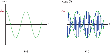
The parameter fc is referred to as the carrier frequency. Note that the phase term ϕc in Eqn. (11.01) is not important for this discussion, and we will simplify the formulation of amplitude modulation without losing any generality by assuming that ϕc = 0. One example of an AM signal is depicted in Fig. 11.4.

Waveforms involved in amplitude modulation: (a) the message signal, (b) the message signal with offset Ac, and (c) the amplitude-modulated carrier and its envelope.
In this particular example we have assumed that the amplitudes of the message signal are constrained to remain in the interval mmin ≤ m(t) ≤ mmax. Further, we will assume that the time average of the signal m(t) is zero. The new amplitude function [Ac + m (t)] will remain in the range
Furthermore, the relationship between Ac and m (t) is chosen such that [Ac + m (t)] ≥ 0 for all t. As a result, the envelope of the modulated carrier, that is, the waveform obtained by connecting the positive peaks of xAM (t), matches [Ac + m (t)]. This will be important as we consider ways of recovering the message signal m (t) from the AM signal xAM (t).
In contrast, consider the example in Fig. 11.5 where [Ac + m (t)] is allowed to be negative for some values of t. In this case the envelope of the AM waveform does not equal [Ac + m (t)], but rather its absolute value |Ac + m (t)|.
![Figure showing Waveforms involved in amplitude modulation when [Ac + m (t)] ≥ 0 is not satisfied for all t : (a) the message signal, (b) the message signal with offset Ac, and (c) the amplitude-modulated carrier and its distorted envelope.](http://imgdetail.ebookreading.net/data/1/9781466598546/9781466598546__signals-and-systems__9781466598546__image__1013x001.png)
Waveforms involved in amplitude modulation when [Ac + m (t)] ≥ 0 is not satisfied for all t : (a) the message signal, (b) the message signal with offset Ac, and (c) the amplitude-modulated carrier and its distorted envelope.
Combining the two cases considered above we obtain a general expression for the envelope of the AM signal as
If [Ac + m (t)] ≥ 0 for all t, then the envelope is a replica of the message signal m (t) subject to a constant offset. Otherwise, the envelope is a distorted version of the message signal. In order to preserve the shape of the message signal in the envelope of the AM signal, we need
Let us define the modulation index as
which can be expressed either as a fraction or as a percentage. For the envelope to display the correct shape of the message signal, we need 0 ≤ μ ≤ 1. An amplitude modulated carrier with a modulation index μ < 1 is said tobe under-modulated. A modulation index of μ = 1 leads to the critically-modulated case. Both of these will allow a simple system known as an envelope detector to be used in recovering the message signal m (t) from the AM signal xAM (t). On the other hand, if μ > 1, the carrier is said to be over-modulated. In this case the envelope is a distorted version of the message signal, and the envelope detector is no longer a viable option for the recovery of m (t). A more complicated synchronous detector will be needed to extract the message.
Interactive Demo: am_demo1
This demo uses the signals in Figs. 11.4 and 11.5. The message signal and the blank carrier are shown on the left side of the graphical user interface. The main graph on the right side displays the modulated carrier computed as in Eqn. (11.03), as well as its envelope given by Eqn. (11.04). A slider control is provided for allowing the modulation index (refer to Eqn. (11.06)) to be varied in the range 0.4 ≤ μ ≤ 1.8. Alternatively, the desired value of the modulation index may be typed into the edit field (the same range restrictions still apply). Note that, in the implementation of this demo, the peak amplitudes mmin and mmax of the message signal are fixed. Change of modulation index μ is facilitated by changing the parameter Ac as dictated by Eqn. (11.06).
- Observe the changes in the AM signal and its envelope as the modulation index μ is varied.
- Pay attention to the envelope crossover that begins just as the modulation index exceeds 1.
am_demo1.m
Sometimes it is insightful to analyze a modulation technique by using a message signal that has a simple analytical description. One particular message signal that can be used in this way is a single tone. Let the modulating signal be
Substituting m (t) in Eqn. (11.03) the corresponding AM waveform is
which can also be written in the form
with the modulation index defined as μ = Am/Ac. The envelope of the modulated carrier is
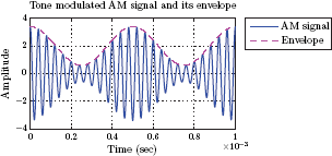
The tone-modulated carrier is shown in Fig. 11.6 for various values of the modulation index. Notice how the envelope is distorted when μ > 1.

Amplitude modulation using a single-tone message signal in Example 11.1: (a) the message signal, (b) under-modulated AM signal with μ = 0.7, (c) critically-modulated AM signal with μ = 1, (d) over-modulated AM signal with μ = 1.5.
ex_11_1.m
Interactive Demo: am_demo2
The demo program “am demo2.m” illustrates amplitude modulation of a carrier by a single tone as discussed in Example 11.1. Three sliders are provided for varying the message frequency fm, the carrier frequency fc, and the modulation index μ. Sliders allow fm to be changed from 0.5 to 3kHz, and fc to be changed from 10 to 25 kHz. Modulation index may be varied between 0.4and 1.8.
- Observe the effect of each change on the AM signal and its envelope.
- See how the envelope crosses over the horizontal axis when the modulation index becomes greater than 1.
- Pay attention to the phase reversal of the carrier at the points of envelope crossover. The easiest method would be to use the “zoom” button in the toolbar at the top of the program window and zoom into the area where envelope crossover occurs.
Software resources:
am_demo2.m
Software resources: |
See MATLAB Exercise 11.1. |
11.4.1 Frequency spectrum of the AM signal
Consider again the expression for an amplitude modulated sinusoidal carrier given by Eqn. (11.03), repeated here for convenience:
Taking the Fourier transforms of both sides, we obtain the frequency spectrum of the AM signal as
where we made use of the modulation theorem of the Fourier transform discussed in Section 4.3.5. The first two terms in Eqn. (11.10) are due to the carrier frequency. The term δ(f + fc) represents an impulse function shifted to the frequency f = −fc. Similarly, δ(f − fc) is an impulse function shifted to the frequency f = fc. The last two terms in Eqn. (11.10) contain shifted versions of the message spectrum. The amount of frequency shift is controlled by the carrier frequency. The term M (f + fc) is a left-shifted version of the message spectrum, and M (f − fc) a right-shifted one. This is depicted in Fig. 11.7.
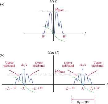
(a) Frequency spectrum M (f) of the message signal; magnitude (solid) and phase (dashed), (b) frequency spectrum XAM (f) of the amplitude-modulated signal; magnitude (solid) and phase (dashed).
Note that the shape of the message spectrum M (f) in Fig. 11.7 is chosen arbitrarily for illustration purposes only; different message signals will have different looking spectra. For positive frequencies, the part of the AM spectrum that occupies frequencies greater than the carrier frequency fc is referred to as the upper sideband. Conversely, the part of the spectrum that occupies frequencies less than fc is referred to as the lower sideband. For the negative side of the frequency axis, these definitions are mirrored. Another interesting point to observe is that, for positive frequencies, lower and upper sidebands occupy the frequency range from fc − W to fc + W. Thus, if the spectrum of the message signal has a one-sided bandwidth of W Hz, then the spectrum of the amplitude-modulated signal has a one-sided bandwidth of BT = 2W Hz, that is, twice the message bandwidth. BT is called the transmission bandwidth of the AM signal.
This illuminates one of the shortcomings of amplitude modulation: It is wasteful of bandwidth. A message signal which occupies a bandwidth of W Hz in its baseband form requires twice that bandwidth when it is embedded into the amplitude of a carrier. We will see in Section 11.6 that single sideband modulation provides a solution to the problem of wasting bandwidth.
The relationship between the carrier frequency fc and the message bandwidth W is also important. To avoid overlaps between spectral components when the message spectrum is shifted right and left, we need fc > W, that is, we need the carrier frequency to be greater than the highest frequency in the message spectrum. Going one step further, if the envelope of the AM signal is required to be a good-quality representation of the message signal, then we need fc >> W, that is, we need the carrier frequency to be significantly greater than the message bandwidth. In practical applications, fc is often several magnitudes greater than W.
The demo program “am_demo3.m” illustrates the frequency spectrum of the AM signal, and is based on Fig. 11.7. The sample message spectrum picked for this demo has a bandwidth of 1 kHz and a peak magnitude of max {|M (f)|} = 1. Amplitude parameter for the carrier is set as Ac = 2. As a result, the modulation index is fixed. A slider control allows the carrier frequency to be varied in the range 2 kHz ≤ fc ≤ 9 kHz. Move the slider to vary the carrier frequency fc, and the observe the effect on the spectrum of the AM signal. Pay attention to the shifting of the spectrum when fc is changed.
Software resources:
am_demo3.m
Example 11.2: Frequency spectrum of the tone-modulated carrier
Compute the frequency spectrum of the tone-modulated AM carrier of Example 11.1 in terms of the carrier frequency fc, the message frequency fm, the modulation index μ and the amplitude Ac.
Solution: Recall that the tone-modulated signal is in the form
which can also be written as
Applying the appropriate trigonometric identity2 to the second term of Eqn. (11.11) we obtain
Eqn. (11.12) contains three sinusoidal terms at frequencies fc, fc + fm and fc − fm respectively. Individual Fourier transforms of the three terms are
Thus, the spectrum of the tone-modulated AM signal is obtained as
Frequency spectra for the single-tone message signal and the amplitude-modulated signal are shown in Fig. 11.8.
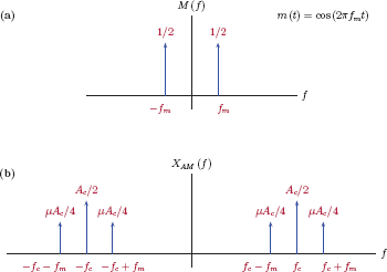
(a) Frequency spectrum M (f) of the single-tone message signal, and (b) frequency spectrum of the tone-modulated AM signal of Example 11.2.
The first two terms in Eqn. (11.13) are due to the carrier alone. The remaining four terms are the sidebands due to the message signal, and they are around positive and negative carrier frequencies with displacements of ±fm in either direction.
Interactive Demo: am_demo4
This demo illustrates the effects of various parameters on the frequency spectrum of the tone-modulated AM signal, and is based on Fig. 11.8 and Eqn. (11.13) of Example 11.2. Use the slider controls to vary the message frequency fm, the carrier frequency fc,and the modulation index μ. Sliders allow fm to be changed from 0.5to3 kHz, and fc to be changed from 10 to 25 kHz. Modulation index may be varied between 0.4 and 1.8. The amplitude is fixed at Ac = 1. Vary the parameters, and observe
- The frequency shifting of the sidebands of the spectrum as the carrier frequency is changed
- How the locations of impulses representing sidebands are related to the message frequency fm and the carrier frequency fc
- The area under each impulse as the modulation index is changed
Software resources:
am_demo4.m
Example 11.3: AM spectrum for a multi-tone modulating signal
Determine the frequency spectrum of the AM signal produced by modulating a carrier at frequency fc = 1 kHz with the two-tone signal
Use the modulation index μ = 0.7.
Solution: First we need to determine the message spectrum. In order to get the phase relationship between the two terms correctly, the sine function in m (t) needs to be converted to a cosine function. Using the appropriate trigonometric identity,3 m (t) can be written as
Using Euler’s formula, Eqn. (11.14) becomes
which yields the spectrum shown in Fig. 11.9.

Frequency spectrum M (f) of the two-tone message signal of Example 11.3: (a) magnitude, (b) phase.
The next step is to determine the carrier amplitude Ac that will yield the desired modulation index value of μ = 0.7. This, in turn, requires the minimum value of the message signal which is found from Eqn. (11.14) to be
and occurs at time instant t = 4.28 ms as shown in Fig. 11.10.
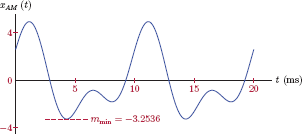
Using Eqn. (11.06) the carrier parameter Ac is found as
Thus, the AM signal is
and is shown in Fig. 11.11(a). The frequency spectrum of the AM signal can be easily found using Eqn. (11.10) along with the message spectrum in Fig. 11.9. The magnitude and the phase spectra of the AM signal are shown in Fig. 11.11(b) and (c).
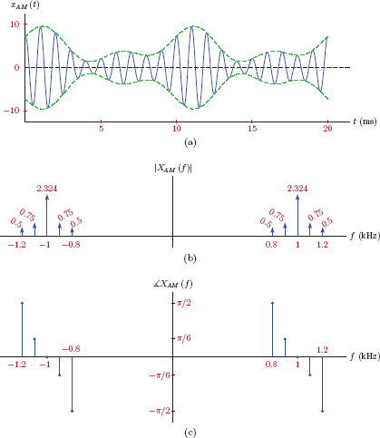
(a) The AM signal for Example 11.3, (b) the magnitude of the frequency spectrum, (c) the phase of the frequency spectrum.
Software resources:
ex_11_3.m
See MATLAB Exercise 11.2. |
Example 11.4: Phasor analysis of the tone-modulated AM signal
The mathematical expression for a carrier with frequency fc that is amplitude-modulated by a single tone with frequency fm was derived in Eqn. (11.08) as
which, using trigonometric identities, can be written as
The first term in Eqn. (11.15) is the carrier term. The remaining two terms are the upper sideband and lower sideband terms terms respectively as we have seen in Fig. 11.8. Let
and
so that the amplitude modulated signal can be written as
In Section 1.3.7 of Chapter 1 we have discussed means of representing sinusoidal signals with phasors. The techniques developed in that section can be applied to the three terms of the AM signal in Eqn. (11.16), Eqn. (11.17), Eqn. (11.18) to obtain
If we wanted to apply the phasor notation of Section 1.3.7 in a strict sense, we would need to express Eqns. (11.20), (11.21) and (11.22) as
The phasor Xcar = Ac ∡0° rotates counterclokwise at the rate of fc Hz, that is, fc revolutions per second. The phasors Xusb = (μAc/2) ∡0° and Xlsb = (μAc/2) ∡0° rotate at the rates of (fc + fm) and (fc − fm) Hz respectively. It is impractical to work with three phasors when each rotates at a different speed. Instead, we will take a slightly unconventional approach and rewrite Eqns. (11.24) and (11.25) as
and
The modified phasors
and
have the same base rotation rate of fc Hz as the phasor Xcar. This allows us to add the three phasors together as vectors. In addition to the base rotation at the rate of fc Hz, each of the modified phasors and has a secondary rotation at the rate of ±fm Hz relative to the carrier phasor Xcar. This is illustrated in Fig. 11.12 for a modulation index of μ < 1.

The phasor Xcar is drawn starting at the origin. The phasors and are shown attached to the tip of the phasor Xcar, and they rotate around the tip of Xcar with speeds of ±fm. The entire system of three phasors rotates around the origin at a speed of fc. The AM signal can be written as
One interesting use of the phasor representation derived above is finding the envelope of the AM signal. In the time domain, we know that the envelope of the AM signal is obtained by connecting the positive peaks of the high-frequency carrier. The equivalent of this action in phasor domain would be to freeze the base rotation (around the origin) of the system of three phasors at a 0-degree angle, and allow only the slower rotations of the phasors and at the rates ±fm Hz around the tip of Xcar. The use of this idea for determining the envelope is shown in Fig. 11.13.

The resulting envelope is
which is consistent with the expression found earlier for μ < 1.
Interactive Demo: am_demo5
This demo illustrates the concepts discussed in Example 11.4. The system of three phasors Xcar, and that make up the phasor description of the AM signal is shown in the upper right part of the graphical user interface. The carrier frequency fc, the singletone message frequency fm and the modulation index μ of the AM signal may each be controlled using the appropriate slider control. The time variable may be advanced using a slider control, and the rotation of the system of phasors may be observed. Pay particular attention to
- The base rotation around the origin, and the slower rotation of the two sideband phasors and around the tip of the carrier phasor Xcar
- How the real part of the vector sum of three phasors corresponds to the amplitude of the AM signal xAM (t) shown in the graph at the bottom
Software resources:
am_demo5.m
Interactive Demo: am_demo6
This demo shows how the system of three phasors discussed in Example 11.4 relates to the envelope of the tone-modulated AM signal. In order to see just the envelope without the carrier, the base rotation of the system of phasors is stopped, that is, the carrier phasor Xcar lays on the horizontal axis without rotating. The sideband phasors and rotate with the frequency fm. In this case, the real part of the vector sum of three phasors corresponds to the envelope of the AM signal.
Software resources:
am_demo6.m
11.4.2 Power balance and modulation efficiency
In the AM signal of Eqn. (11.03), the first term Ac cos(2πfctt), referred to as the carrier component, is independent of the message signal. The sole purpose of transmitting the carrier component along with the message-dependent second term is to ensure that the envelope of the resulting signal resembles the message signal. From a power perspective, the transmission of the carrier component represents a waste of power. In contrast, the second term in Eqn. (11.03) includes the message signal m (t), and thus represents the useful component of the AM signal. It would be interesting to find what percentage of the power in the transmitted AM signal is useful, and what percentage is wasted. The normalized average power of the AM signal is
where the 〈...〉 operator indicates time averaging as we have discussed in Section 1.3.5 of Chapter 1. Using the appropriate trigonometric identity,4 Eqn. (11.31) can be written as
Assuming that the carrier frequency is significantly greater than the bandwidth of the message signal, the second term in Eqn. (11.31) averages to zero, and we have
For most message signals m (t) = 0, and Eqn. (11.32) reduces to
The first term in Eqn. (11.33), , is the power in the carrier component, that is, the wasted power. In contrast, the second term is the power in the sidebands, or the useful power. We will define the modulation efficiency as the percentage of the useful power within the total power of the AM signal:
As expected, modulation efficiency depends on the significance of next to 〈m2 (t)〉. For practical message signals, lower and upper bounds of the allowable amplitude range are often symmetric, that is, |mmin| = |mmax|. For the case μ ≤ 1, this would lead to
As a result, the numerator term is bound by
with the equality achieved only when the message signal is in the form of a square-wave type signal with amplitudes of ±Ac only. Thus, the maximum theoretical efficiency that can be attained with amplitude modulation (when the envelope is preserved) is η = 0.5, or 50 percent. Actual efficiency values obtained in practice will be significantly lower.
In summary, amplitude modulation is wasteful of power. This is the second major shortcoming of amplitude modulation besides the issue of inefficient bandwidth utilization discussed in the previous section.
Example 11.5: Efficiency in tone modulation
Determine the modulation efficiency for the tone-modulated AM signal of Example 11.1.
Solution: Recall that the modulating signal was given by
Thus, the average normalized power of the message signal is
Using this result in Eqn. (11.33) we find the modulation efficiency of a tone-modulated AM signal to be
In the case of tone-modulation, the maximum efficiency that can be achieved while preserving the signal envelope is η = 0.333, or 33.3 percent for the critically-modulated case μ = 1. For smaller values of μ the efficiency will be even lower.
Example 11.6: Multi-tone modulating signal revisited
Determine the power efficiency of the AM signal of Example 11.3.
Solution: Recall that the AM signal obtained in Example 11.3 was
The average normalized power in the message signal is
The average normalized power of the AM signal including the carrier is
Power efficiency is found as the ratio of the two results:
11.4.3 Generation of AM signals
Consider again the basic form of the AM signal given by Eqn. (11.03). Theoretically it is possible to produce this signal by using a product modulator as shown in Fig. 11.14.

The system uses an analog multiplier, an analog adder, and an amplifier. An oscillator generates the sinusoidal carrier signal cos (2πfctt). The message signal and the carrier signal are first multiplied to obtain the second term of Eqn. (11.03). Afterwards, a properly scaled version of the carrier signal is added into the mix to complete the AM signal. The adder and the amplifier in Fig. 11.14 can be implemented easily; however, multiplication of two analog signals in time is an operation that is only practical at relatively low power levels. Radio broadcast stations produce AM signals at power levels typically in the 10 to 50 kW range. Implementation of analog multipliers is impractical at such power levels, hence we need to look into alternative means of generating high-power AM signals. We will consider two of these alternatives, namely a switching modulator, and a square-law modulator.
Switching modulator
Consider the arrangement shown in Fig. 11.15 where the carrier signal xc (t) = Bc cos (2πfctt) and the message signal m (t) are added together, and their sum is applied to a diode rectifier that consists of a diode and a resistor.

Ideally, the role of the diode rectifier would be to replace negative signal amplitudes with zero while keeping positive amplitudes unchanged. It is assumed that the amplitude of the sum signal is large enough for the diode to be modeled as an ideal switch. Furthermore, we will ensure that the amplitude of the carrier term within the sum is significantly greater than the message term, that is, Bc >> m (t), so that the switching action of the diode and resistor combination is controlled largely by the carrier term alone. With these assumptions, the combination of the diode and the load resistor can be modeled as an ideal switch with the characteristic as shown in Fig. 11.16

The input to the switching circuit with the diode and the load resistor is
and the output voltage of the switching circuit is
The assumption Bc >> m (t) ensures that the switching action in Eqn. (11.37) is controlled by xc (t), and the effect of the message signal m (t) on switching is negligibly small. Mathematically, the switching relationship in Eqn. (11.37) is equivalent to multiplying vi (t) with a hypothetical pulse train:
This relationship is depicted in Fig. 11.17.

The pulse train p (t) is periodic with the same period Tc = 1/fc as the carrier, and it has a duty cycle of d = 0.5. (The assumption Bc >> m (t) that we made earlier was needed for this purpose.) The sinusoidal carrier is shown in Fig. 11.17 with dashed lines to illustrate its relationship to the pulse train p (t). An alternative yet equivalent perspective is given in Fig. 11.18 where the relationship in Eqn. (11.38) is implemented in the form of an electronic switch controlled by the pulse train p (t).
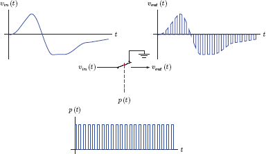
For the duration of each pulse, that is, when p (t) = 1, the switch is in the top position, connecting the signal vin (t) to the input of the bandpass filter. Between pulses, the switch is in the lower position, grounding the input of the bandpass filter. The TFS representation of the pulse train p (t) in Eqn. (11.38) is (see Section 4.2.2 of Chapter 4)
Note that the fundamental frequency in Eqn. (11.39) is the same as the carrier frequency fc. The coefficients of the Fourier series expansion are found as
Using Eqn. (11.39), Eqn. (11.39), Eqn. (11.41) along with Eqn. (11.37), we can write Eqn. (11.38) as
or as
The purpose of the bandpass filter in Fig. 11.15 becomes apparent from Eqn. (11.43). The first two terms are at low frequencies: Bc/π is a constant, and has frequencies extending up to W Hz. The next two terms correspond to an AM signal, and they are the terms we need to keep so that we have
The remaining terms in Eqn. (11.42) are at higher frequencies. The bandpass filter is needed to eliminate the undesired low-frequency and high-frequency terms. It needs to be designed such that the content in the frequency range
is kept, and the frequencies outside that range are eliminated. Also, in order to avoid any overlap between the spectrum of the AM signal and the spectra of low-frequency terms, we need fc > 2W. This is not a very restricting requirement since, in most practical cases, fc >> W. In Eqn. (11.44), the parameter Bc can be adjusted to obtain the desired modulation index. Comparing Eqn. (11.44) with Eqn. (11.08) it is obvious that Ac = Bc/2, and the modulation index can be determined by
Interactive Demo: am_demo7
This demo program implements a simulation of the switching modulator discussed above. Implementation is based on Eqn. (11.36), Eqn. (11.37), Eqn. (11.38), Eqn. (11.39), Eqn. (11.40), Eqn. (11.41), Eqn. (11.42), Eqn. (11.43), Eqn. (11.44), Eqn. (11.45), using a single-tone modulating signal m (t) = cos(2πfmtt). The parameters Bc, fc and fm are adjustable through the use of slider controls in the interface. The undesired terms of Eqn. (11.43) are filtered out using a fifth-order Butterworth bandpass filter. The passband edge frequencies f1 and f2 of this filter (refer to MATLAB Example 11.3) are controlled indirectly by means of a center frequency fb and a passband width fv so that the lower edge of the passband is at
and its higher edge is at
It should be understood that, by “edge frequency” for a Butterworth filter, we are referring to a frequency where the magnitude of the system function decreases from its peak value by 3 dB.
The modulation index that results from this process is given by Eqn. (11.45). For the single-tone modulating signal used in this case max {|m (t)|} = 1, and Eqn. (11.45) reduces to
which is displayed as the parameter Bc is varied. The signals vin (t), vout (t), and are computed and graphed. Additionally, the ideal envelope
is displayed superimposed with for comparison. Vary the simulation parameters and observe the following:
- The relationship between the modulation index μ and the carrier amplitude Bc
- The summing of the carrier and the message signals to obtain the signal vin (t)
- The relationship between the signals vin (t) and vout (t)
- The time lag between the ideal envelope and the synthesized AM signal that is due to the Butterworth bandpass filter
- The effect of the edge frequencies of the Butterworth filter on the quality of the synthesized signal and on the time lag
- The relationship between fc, fm, and the bandpass filter edge frequencies as dictated by Eqn. (11.43)
am_demo7.m
Software resources: |
See MATLAB Exercises 11.3 and 11.4. |
Square-law modulator
The basis of a square-law modulator is a nonlinear device with a strong second-order nonlinearity. Consider an ideal second-order nonlinear device with the following input-output characteristic:
In practice, a diode or a transistor operating in small-signal mode would produce a characteristic that is fairly close to Eqn. (11.46). As in the case of the switching modulator, let the input voltage to this nonlinear device be the sum of the carrier and the message signal:
Using Eqn. (11.47) in Eqn. (11.46), the output voltage of the nonlinear device is found to be
which can be written as
In Eqn. (11.49) we recognize the first and the last terms as the ones that we need for an amplitude modulated carrier. The three terms in between are the terms that we will need to eliminate. Let us rearrange Eqn. (11.49) by combining the useful terms together to obtain
It is obvious that the first term is the AM signal with Ac = aBc and μ = 2b/a. The remaining terms need to be eliminated to yield an amplitude-modulated signal
In order to find a way to eliminate the undesired terms, we need to understand what range of frequencies each term occupies in the frequency spectrum of vout (t). Assuming that the message signal m (t) has a bandwidth of W, frequency ranges of individual terms of Eqn. (11.50) are detailed in Table 11.1.
Terms in Eqn. (11.50) and the frequencies they occupy.
Index |
Term |
Frequencies |
|---|---|---|
1 |
a Bc [1 + (2b/a)m(t)] cos(2πfct) |
fc − W ≤ f ≤ fc + W |
2 |
a m (t) |
− W ≤ f ≤ W |
3 |
f = 0, and f = 2fc |
|
4 |
b m2 (t) |
− 2W ≤ f ≤ 2W |
The frequency spectrum of vout (t) is shown in Fig. 11.19. The terms of the spectrum are numbered based on their indices in Table 11.1.

An inspection of the spectrum in Fig. 11.19 reveals that the amplitude modulated carrier may be isolated and the undesired terms may be removed by processing the signal vout (t) through a bandpass filter. Thus, the square-law modulator is completed by connecting an appropriate bandpass filter to the output of the nonlinear device. A block diagram for it is shown in Fig. 11.20.

Interactive Demo: am_demo8
This demo provides a simulation of the square-law modulator considered in Fig. 11.20, Eqn. (11.46), Eqn. (11.47), Eqn. (11.48), Eqn. (11.49), Eqn. (11.50). As in the demo program “am_demo7.m”, a single-tone modulating signal m (t) = cos(2πfmt) is used. Parameters encountered in square-law modulator discussion above, namely fc, fm,a and b, may be adjusted using the slider controls provided. The signals vin (t) and vout (t) are computed by direct application of Eqns. (11.47) and (11.48) respectively. Afterwards, the signal is computed by processing the signal vout (t) through a fifth-order Butterworth bandpass filter with user-specified critical frequencies f1and f2 which are again specified indirectly by means of parameters fb and fv as
The effect of the parameter Bc on the modulator output signal is relatively insignificant; therefore this parameter is fixed as Bc = 1. The three signals vin (t), vout (t) and are graphed. The modulation index for the synthesized signal is given by μ = 2b/a, and is displayed as the parameters a and b are varied. The ideal envelope
is displayed superimposed with for comparison. Vary the simulation parameters and observe the following:
- The relationship between the modulation index μ and the parameters a and b of the nonlinear characteristic
- The relationship between the signals vin (t) and vout (t)
- The time lag between the ideal envelope and the synthesized AM signal that is due to the Butterworth bandpass filter
- The effect of the edge frequencies of the Butterworth filter on the quality of the synthesized signal and on the time lag
- The relationship between fc, fm, and the bandpass filter edge frequencies as dictated by Table (11.1)
Software resources:
am_demo8.m
Software resources: |
See MATLAB Exercises 11.5 and 11.6. |
11.4.4 Demodulation of AM signals
The term demodulation refers to the act of recovering the message signal m (t) as closely to its original form as possible from the modulated waveform xAM (t). It was illustrated in Figs. 11.4 and 11.5 that, as long as the modulation index is less than 100 percent, the envelope of the modulated carrier resembles the message signal. In that case the simplest means of demodulation is by using an envelope detector.
Envelope detector
Consider the simple circuit that consists of a diode, a capacitor and a resistor as shown in Fig. 11.21.
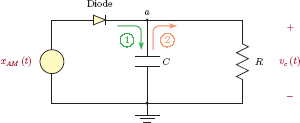
The modulated carrier is applied to this circuit in the form of a voltage signal. The output voltage approximately tracks the envelope of the AM waveform as we will illustrate. Two cases need to be considered:
Case 1: xAM (t) ≥ vc (t)
At time instants when the amplitude of the AM waveform is greater than or equal to the capacitor voltage, the diode of the envelope detector circuit is forward biased, and it conducts current. If we assume an ideal diode with no voltage drop between its terminals, the capacitor charges quickly to maintain vc (t)= xAM (t). This corresponds to current path labeled (1) in Fig. 11.21.
Case 2: xAM (t) < vc (t)
At time instants when the amplitude of the AM waveform is less than the capacitor voltage, the diode becomes reverse biased, and therefore no current flows through it. The capacitor that was charged to the peak value of the carrier must now discharge through the resistor. The discharge current follows the path labeled (2) in Fig. 11.21. Let the peak value of the carrier be vc (t0) = V0 just before the capacitor begins its discharge at time t = t0. We know that the current of the capacitor is related to its voltage by ic (t)= C dvc (t)/dt. Writing Kirchhoff’s current law at the node labeled “a”, we have
which leads to the differential equation that governs the discharge of the capacitor:
subject to the initial condition vc (t0)=V0. The solution of this differential equation is in the form
where V0 is the initial value at the beginning of the discharge cycle, that is, the peak value of the carrier at the point it switches from case 1 to case 2. This behavior of the envelope detector is illustrated in Fig. 11.22.

The time constant of the discharge is τ = RC. It is important to note that the rate of decay for the exponential solution in Eqn. (11.54) is critical for the proper operation of the envelope detector. Thus, the time constant must be chosen carefully. If vc (t) decays too rapidly, the resulting envelope will look quite busy with too much high-frequency detail. If, on the other hand, vc (t) decays too slowly, then output will have sections where it deviates significantly from the correct envelope behavior as illustrated in Fig. 11.23.
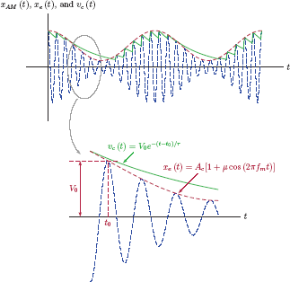
We will address the problem of finding a proper value of τ in Example 11.7.
Example 11.7: Envelope detector for tone-modulated AM signal
Consider the envelope detector of Fig. 11.21 with a tone-modulated AM waveform as the input signal. Determine the range of the time constant τ needed to properly recover the single-tone message signal from the modulated waveform.
Solution: The envelope detector fills the gaps between the peaks of the carrier with decaying exponential voltage segments due to the discharging behavior of the RC circuit. In this process, the critical parameter is the time constant τ of the discharge. It was illustrated in Fig. 11.23 that, if the time constant is too large, the envelope detector output voltage fails to track the actual envelope. This happens because the slope of the actual envelope is more negative than the slope of the exponential discharge. Therefore, it would make sense to compare the slopes of the actual envelope and the exponential discharge to come up with the necessary condition that must be imposed on the choice of τ. We will begin with the actual envelope which, for the tone-modulated case, is
with the assumption that μ < 1. The slope of the envelope is
Let us pick a time instant t = t0 at one of the peaks of the carrier as shown in Fig. 11.22. At that instant, the slope of the envelope is
The envelope detector output right after thetimeinstant t = t0 is
and the slope of the envelope detector output is
Evaluating this slope at t = t0 where it is maximum, we obtain
Now we are ready to state the condition for the envelope detector output to correctly track the envelope of the AM signal. We need the slope in Eqn. (11.60) to be more negative than the value in Eqn. (11.57):
Let α ≜ 2πfmt0 to simplify the notation, and Eqn. (11.61) becomes
or equivalently
It is important for the inequality in Eqn. (11.63) to be satisfied for all values of α, including when the right side has its smallest possible value. To determine the minimum value of the expression in parentheses, we need to differentiate it with respect to α and set the result equal to 0. This yields cos(α) = −μ and, consequently, . Substituting these into Eqn. (11.63) we obtain
The time constant τ = RC should satisfy the inequality in Eqn. (11.64) in order to avoid the loss of tracking for the envelope detector. The result we have derived is for the case when the modulating signal is a single tone. If the modulating signal has a range of frequencies, then Eqn. (11.64) can still be used heuristically, and the inequality should be satisfied for the highest frequency in the message signal, i.e.,
Interactive Demo: am_demo9
This demo is based on Example 11.7. It simulates an envelope detector used on an AM signal modulated by a single-tone message signal. Carrier frequency fc, message frequency fm, modulation index μ, and envelope detector time constant τ may be adjusted by using the slider controls provided. The program computes and graphs the AM waveform, the correct envelope, and the envelope detector output for the parameter values specified. The minimum time constant needed for proper detection of the envelope is computed using Eqn. (11.65), and is displayed.
- Observe the dependency of the maximum time constant on the modulation index μ and the message frequency fm.
- Explain why the maximum time constant is not dependent on the carrier frequency fc.
- Push the time constant beyond its maximum value, and observe the envelope detector output. At what part of the signal does the envelope detector stop tracking the correct envelope?
Software resources:
am_demo9.m
Coherent demodulation
The simple demodulation technique discussed in the previous section only works if the modulation index is less than 100 percent. For μ> 1 we have seen that the envelope of the modulated carrier is a distorted version of the message signal, and is therefore not useful in the demodulation process. The alternative is to use coherent demodulation which requires the availability of a local carrier signal synchronized with the original carrier signal that was used in generating xAM (t). Consider the block diagram shown in Fig. 11.24.
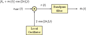
The product r (t) at the output of the multiplier is
Using the appropriate trigonometric identity Eqn. (11.66) can be written as
Using the sample message spectrum M (f) and the corresponding AM signal spectrum XAM (f) shown in Fig. 11.7 the spectrum of the intermediate signal r (t) isasshown in Fig. 11.25.
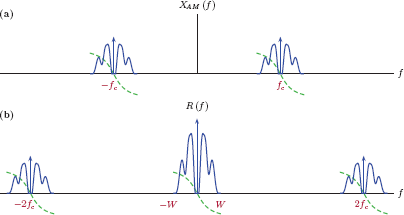
Frequency spectrum R (f) of the intermediate signal in the coherent demodulator shown in Fig. 11.24.
It is clear from Fig. 11.25 that, in order to recover the message spectrum M (f) from R (f) the high frequency component around 2fc and the dc component should be removed (we are assuming that the message signal m(t) does not have a dc component). That is the role of the bandpass filter.
11.5 Double-Sideband Suppressed Carrier Modulation
In Section 11.4.2 we have seen that one of the shortcomings of amplitude modulation is the amount of power wasted on transmitting the carrier along with the two sidebands. Modulation efficiency given by Eqn. (11.33) is theoretically limited to 50 percent, and is much lower in practice. Less than half the transmitted power is used on information bearing signals, and the rest of the power is wasted for transmitting the carrier.
One method of fixing this shortcoming is to simply drop the power-wasting term Ac cos (2πfct) from the AM waveform expression in Eqn. (11.03). This results in the signal
which is referred to as the double-sideband suppressed-carrier (DSB-SC) modulated signal. In the remainder of this text, we will refer to this signal simply as the DSB modulated signal. Fig. 11.26 illustrates the DSB signal in the time domain.

Waveforms involved in DSB modulation: (a) the message signal, (b) the DSB modulated carrier.
The power efficiency of the DSB modulated signal is 100 percent since no power is being wasted on any non-information-bearing signal components. On the other hand, a comparison of Fig. 11.26 to Fig. 11.4 makes it clear that the envelope is lost in the case of DSB modulation, so we can no longer rely on the simplicity of an envelope detector for recovering the message signal from the modulated signal. A demodulation technique with higher complexity must be employed instead. Specifically, at the receiver end of the communication system, we will need a carrier the frequency and the phase of which are in perfect synchronization with the original carrier used in creating the DSB modulated signal (coherent demodulation). This is the price paid for improved power efficiency.
Interactive Demo: dsb_demo1
This demo uses the signals in Fig. 11.26. The message signal and the blank carrier are shown on the left side of the graphical user interface. On the right side of the graphical user interface, the DSB modulated signal is shown as computed by Eqn. (11.68). A slider control and an edit control are provided for changing the carrier frequency fc.
- Observe the changes in the DSB signal as the carrier frequency fc is varied.
- Notice that the envelope no longer resembles the message signal m (t).
- Pay attention to the 180-degree phase reversal of the carrier at the point of envelope crossover.
Software resources:
dsb_demo1.m
Example 11.8: Tone modulation with DSB
Determine and graph the DSB-SC signal when the modulating signal is a single tone in the form
Solution: Using the specified m (t) the resulting DSB modulated signal is
which is shown in Fig. 11.27.
DSB-SC modulation using a single-tone message signal in Example 11.8: (a) message signal, (b) DSB-SC signal.
The positive envelope of the DSB signal is
As expected, it no longer resembles the message signal m (t).
Software resources:
ex_11_8.m
Interactive Demo: dsb_demo2
This demo is based on Example 11.8 and Fig. 11.27. The DSB modulated signal is graphed with the single-tone modulating signal as given by Eqn. (11.69). Slider controls are provided for changing the values of the message amplitude Am, the single-tone message frequency fm, and the carrier frequency fc. Observe the following:
- The relationship between the message signal m (t) and the positive envelope xe(t) of the DSB signal
- The effects of changing fc and fm
- The 180-degree phase change that occurs in the carrier when the envelope crosses over the horizontal axis
Software resources:
dsb_demo2.m
11.5.1 Frequency spectrum of the DSB-SC signal
The mathematical expression for the double-sideband suppressed-carrier signal was given by Eqn. (11.68). Taking the Fourier transform of both sides of Eqn. (11.68) and using the modulation property discussed in Section 4.3.5 yields
which is illustrated in Fig. 11.28.

(a) Frequency spectrum M (f) of the message signal; magnitude (solid) and phase (dashed), (b) frequency spectrum XDSB (f) of the double-sideband suppressed carrier; magnitude (solid) and phase (dashed).
A quick comparison of Fig. 11.28 and Eqn. (11.71) with their counterparts for amplitude modulation in Section 11.4.1, namely Fig. 11.7 and Eqn. (11.10), reveals that the only difference is the absence of the impulses at ±fc from the DSB-SC spectrum. Upper and lower sidebands are present as before. The transmission bandwidth, BT = 2W, is also unchanged.
Interactive Demo: dsb_demo3
This demo follows Fig. 11.28 and Eqn. (11.71). The spectrum of a sample message signal, and the spectrum of the corresponding DSB-SC signal are shown. The sample message spectrum picked for this demo has a bandwidth of 1 kHz and a peak magnitude of max {|M (f)|} = 1. A slider control is provided for adjusting the carrier frequency fc in the range 2 kHz ≤ fc ≤ 9kHz.
- Observe how the sidebands move inward or outward as the carrier frequency is changed.
- Compare the spectrum of the DSB signal to that of the AM signal in Fig. 11.7 and MATLAB demo am_demo3.m.
Software resources:
dsb_demo3.m
Example 11.9: Frequency spectrum of the tone-modulated DSB-SC signal
Determine and graph the frequency spectrum of the tone-modulated DSB-SC signal.
Solution: The expression for a tone-modulated DSB signal was given in Eqn. (11.69). Using the appropriate trigonometric identity it can be written as
Eqn. (11.72) contains two cosine terms at frequencies fc + fm and fc − fm. For the tone-modulated case these two cosine terms constitute the upper and the lower sideband respectively. Individual Fourier transforms of the two terms in Eqn. (11.72) are
and the spectrum of the tone-modulated DSB signal is obtained as
Frequency spectra for the single-tone message signal and the amplitude-modulated signal of Eqn. (11.73) are shown in Fig. 11.29.

(a) Frequency spectrum M (f) of the single-tone message signal, and (b) frequency spectrum of the tone-modulated DSB-SC signal of Example 11.9.
The DSB spectrum for a single tone modulating signal is similar to the spectrum of the AM carrier with the same modulating signal which was shown in Fig. 11.8. The main difference is the lack of impulses at frequencies ±fc.
Interactive Demo: dsb_demo4
This demo illustrates the concepts explored in Example 11.9 and Fig. 11.29. The two graphs show the spectrum of the single-tone message signal m (t) = Am cos (2πfmt) and the spectrum of the corresponding DSB-SC signal. Slider controls allow adjustments to the message amplitude Am, the message frequency fm and the carrier frequency fc.
- Pay attention to the frequency shift of the sidebands of the spectrum as the carrier frequency is changed.
- Observe how the sideband impulses move toward each other or away from each other as the message frequency is changed.
- Observe the values of the impulses as the message amplitude is changed.
Software resources:
dsb_demo4.m
11.6 Single-Sideband Modulation
One of the shortcomings of amplitude modulation, namely the power efficiency, was addressed in Section 11.5. Dropping the carrier term is the method of improving the power efficiency at the expense of giving up the envelope that resembles the message signal, and the opportunity for simple non-coherent detection afforded by it. Another shortcoming of amplitude modulation is the doubling of the bandwidth. For a message signal with bandwidth W Hz, the transmission bandwidth of both the AM and the DSB-SC waveforms is BT = 2W as is evident from Figs. 11.7 and 11.28.
Consider a message signal m (t) with the frequency spectrum M (f) shown in Fig. 11.30.
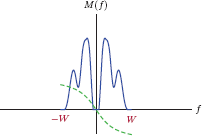
The message signal m (t) is real-valued. Based on the discussion in Section 4.3.5, its frequency spectrum M (f) exhibits conjugate symmetry:
As a result, the magnitude of the spectrum M (f) is an even function of frequency, and the phase of it is an odd function of frequency
and
Let us split the message spectrum into two parts defined as
and
so that M (f) = Mn (f) + Mp (f). Clearly, Mn (f) represents the part of the message spectrum for negative frequencies, that is, the left side. Conversely, Mp (f) represents the right side. This is illustrated in Fig. 11.31.

Based on the symmetry properties outlined in Eqn. (11.74), Eqn. (11.75), Eqn. (11.76), one of the two components of the spectrum, either Mn (f) or Mp (f), makes the other term redundant. For example, if we know Mp (f), we can obtain Mn (f) as
As a result, the transmission of a modulated signal with just one of the sidebands in it is sufficient for the receiver to get the message signal. This is referred to assingle-sideband (SSB) modulation.
Recall that the spectrum of the DSB-SC signal was given by Eqn. (11.71), and includes both lower and upper sidebands. The DSB spectrum can be rewritten using the two components of M (f) as
A single-sideband spectrum can be formed by retaining either the upper sidebands or the lower sidebands. If the upper sidebands are retained, the resulting spectrum is
We will refer to XSSB,U (f) as the upper-sideband SSB spectrum. Alternatively, we can retain the lower sidebands to obtain
which is the lower-sideband SSB spectrum. Fig. 11.32 illustrates the results obtained in Eqn. (11.80), Eqn. (11.81), Eqn. (11.82).
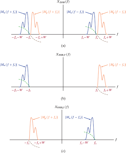
(a) The frequency spectrum of a DSB-SC signal expressed using the spectral components Mn (f) and Mp (f), (b) the upper-sideband SSB spectrum XSSB,U (f), (c) the lower-sideband SSB spectrum XSSB,L (f).
The time-domain signals that correspond to the two SSB spectra of Eqns. (11.81) and (11.82) would be
Theoretically, the SSB signals xSSB,U (t) and xSSB,L (t) can be obtained from the DSB signal xDSB (t) through sideband filtering as illustrated in Fig. 11.33.
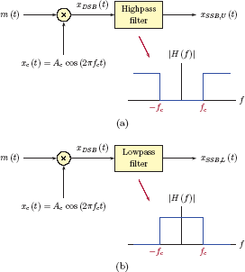
Obtaining SSB signals from the DSB signal through sideband filtering: (a) block diagram for obtaining the upper-sideband SSB signal, and (b) block diagram for obtaining the lower-sideband SSB signal.
The block diagrams in Fig. 11.33 assume that the filters used have ideal characteristics. This approach is not used in practical implementation of SSB modulation since ideal filters are not available and would be near impossible to approximate since the allowed transition band would be extremely narrow relative to the carrier frequency.
One question that we have not yet considered up to this point is:What does the time-domain SSB signal look like? We will use Eqns. (11.81) and (11.82) to derive time-domain expressions for the lower-sideband and upper-sideband SSB signals. The message signal m (t) can be writteninthe form
where mn (t) and mp (t) are the time-domain signals that correspond to the two components of the spectrum, Mn (f) and Mp (f), respectively:
Using the frequency-shifting property of the Fourier transform, time-domain equivalents of Eqns. (11.81) and (11.82) can be derived as
Let us first consider mp (t) and its Fourier transform Mp (f). The transform Mp (f) is nonzero only for positive frequencies, and is not conjugate symmetric. As a result, we expect the time-domain signal mp (t) to be complex-valued. One way of relating the transform Mp (f) to the message spectrum M (f) is through the use of the signum function:
Consider a signal derived from m (t) and M (f) through the Fourier transform relationship
The Fourier transform of is
The signal is known as the Hilbert transform of the signal m (t). It can be modeled as the output signal of a Hilbert transform filter with system function
driven by the message signal m (t) as illustrated in Fig. 11.34.

Hilbert transform of the signal m (t) modeled as the output of a Hilbert transform filter.
Substituting Eqn. (11.92) into Eqn. (11.90) we obtain
and
Mathematical expressions for the left half of the spectrum and the corresponding time-domain signal can also be obtained through similar derivations:
We are now ready to write the time-domain expressions for the upper-sideband SSB and lower-sideband SSB signals in terms of the message signal. Substituting Eqn. (11.95), Eqn. (11.96), and Eqn. (11.97) into Eqn. (11.88) yields the the expression for the upper-sideband SSB signal as
which can be simplified to
Similarly, the lower-sideband SSB signal can be found by substituting Eqn. (11.95), Eqn. (11.96), and Eqn. (11.97) into Eqn. (11.89), and simplifying the result.
11.7 Further Reading
[1] L.W. Couch.Digital and Analog Communication Systems. Always Learning. Prentice Hall, 2013.
[2] B.P. Lathi and Z. Ding.Modern Digital and Analog Communication Systems. The Oxford Series in Electrical and Computer Engineering. Oxford University Press, 2009.
[3] J.G. Proakis, M. Salehi, and G. Bauch.Contemporary Communication Systems Using MATLAB, 3rd ed. Cengage Learning, 2011.
MATLAB Exercises
MATLAB Exercise 11.1: Compute and graph the AM signal
Develop a MATLAB script for generating samples of the tone-modulated AM signal given by Eqn. (11.08), using parameter values fc = 25 kHz, fm = 2 kHz, Ac = 2, and μ = 0.7. Graph the resulting signal.
Solution: An important issue is the time increment used in evaluating amplitude values of the AM signal. Even though our final graph will mimic the behavior of an analog signal, it is obvious that any signal we generate with MATLAB is discrete by nature. In essence, we will be sampling the analog AM signal of Eqn. (11.08) to produce a discrete-time signal, and then graphing it to look like an analog signal. The time increment used in the calculation of AM signal values is the same as the sampling interval Ts = 1/fs discussed in Chapter 6. It needs to be chosen sufficiently small compared to the period of the carrier so that the resulting graph is an accurate representation of the AM signal. Nyquist sampling theorem states that the sampling rate fs needs to be at least twice the highest signal frequency. In this example, however, we will go well beyond that requirement so that the resulting analog graph looks smooth. For the parameter values chosen, the highest frequency in the signal xAM (t) is fc + fm = 27 kHz. We will choose the time increment as Ts = 10−6 seconds, corresponding to a sampling rate of fs = 1 MHz. MATLAB code is listed below.
1 % Script: matex_11_1.m
2 %
3 Ac = 2;
4 Mu = 0.7;
5 fc = 25000;
6 fm = 2000;
7 t = [0:1e-6:1e-3]; % Vector of time instants.
8 % Compute the AM signal.
9 x_am = Ac*(1+ Mu*cos(2*pi*fm*t)).*cos(2* pi* fc*t); % Eqn. (11.08)
10 % Compute the envelope.
11 x_env = abs(Ac*(1+ Mu* cos(2*pi* fm*t))); % Eqn. (11.09)
12 % Graph the AM signal and the envelope.
13 clf;
14 plot (t, x_am,'-',t, x_env ,'m--'),
15 grid;
16 title ('Tone modulated AM signal and its envelope'),
17 xlabel ('Time (sec)'),
18 ylabel ('Amplitude'),
19 legend ('AM signal', 'Envelope'),
The graph that is generated by the script matex_11_1.m is shown in Fig. 11.35.
Software resources:
matex_11_1.m
MATLAB Exercise 11.2: EFS spectrum of the tone-modulated AM signal
Refer to the tone-modulated AM signal graphed in MATLAB Exercise 11.1. Determine its fundamental period. Afterwards compute and graph its EFS spectrum.
Solution: First we need to determine the periodicity of the signal. With parameter values fc = 25 kHz and fm = 2 kHz, the frequencies contained in the AM signal are fc = 25 kHz, fc − fm = 23 kHz and fc + fm = 27 kHz. The fundamental frequency of the signal xAM (t) is f0 = 1 kHz corresponding to a fundamental period of T0 = 1 ms (see the discussion in Section 1.3.4 of Chapter 1). The script listed below computes samples of exactly one period of the tone-modulated AM signal and then uses the function ss_efsapprox(..) developed in MATLAB Exercise 5.13 of Chapter 5 to approximate the EFS line spectrum of the signal.
1 % Script : matex_11_2.m
2 %
3 Ac = 2;
4 Mu = 0.7;
5 fc = 25000;
6 fm = 2000;
7 t = [0:999]*1e-6;
8 x_am = Ac*(1+Mu*cos(2*pi*fm*t)).*cos(2*pi*fc*t);
9 clf;
10 k =[-30:30];
11 ck = ss_efsapprox(x_am ,k);
12 stem (k, ck);
13 title ('EFS coefficients for x_{AM}(t)'),
14 xlabel ('Index k'),
The graph that is generated by the script matex_11_2.m is shown in Fig. 11.36.

Software resources:
matex_11_2.m
MATLAB Exercise 11.3: Function to simulate a switching modulator
In this example, we will develop a MATLAB function to simulate the behavior of the switching modulator discussed. In MATLAB, the switching behavior in Eqn. (11.37) can be implemented with the following statements:
>> control = (carrier >= 0);
>> v_out = v_in.*control;
The two statements may also be combined as
>> v_out = v_in.*(carrier >= 0);
The next step is to use a bandpass filter for cleaning up the undesired terms. Function butter(..) will be used for designing a suitable bandpass filter for this purpose (see MATLAB Exercises 10.1, 10.9 and 10.10 in Chapter 10).
>> [numz, denz] = butter(N,Wn, 'bandpass'),
Once a suitable bandpass filter is designed, function filter(..) is used for processing the switched signal through it. The listing for the function ss_switchmod(..) is given below. The input arguments to the function are
Vector holding samples of the message signal. |
|
Bc: |
Amplitude of the carrier to be added to the message signal. |
fc: |
Carrier frequency in Hz. |
Ts: |
Time increment in seconds, used for the message signal in vector “msg”, and also in computing samples of the synthesized AM signal. |
f1: |
Lower edge frequency in Hz for the bandpass filter. |
f2: |
Upper edge frequency in Hz for the bandpass filter. |
The function returns a vector holding the samples of the synthesized AM waveform.
1 function x_am = ss_switchmod(msg, Bc, fc, Ts, f1, f2)
2 nSamp = length (msg); % Number of samples in "msg"
3 t = [0:nSamp-1]*Ts; % Vector of time instants
4 carrier = Bc*cos (2*pi*fc*t);
5 % Compute input to the diode switch.
6 v_in = carrier + msg; % Eqn. (11.36)
7 % Simulate the diode switch.
8 v_out = v_in.*(carrier >=0); % Eqn. (11.37)
9 % Design the bandpass filter.
10 [numz, denz] = butter (5,[2*f1*Ts,2*f2*Ts], 'bandpass'),
11 % Process switch output through bandpass filter.
12 x_am = filter (numz, denz, v_out);
It is important to understand the relationship between analog frequencies in Hz and the normalized frequencies used in bandpass filter design. Given the frequency interval f1 < f < f2 Hz that we would like to retain and a sampling rate of fs used in the simulation, the normalized edge frequencies of the bandpass filter are
Since MATLAB defines normalized frequencies differently (see Chapter 10), the values used in the call to function butter(..) are 2F1 = 2f1/fs and 2F2 = 2f2/fs.
Software resources:
ss_switchmod.m
MATLAB Exercise 11.4: Testing the switching modulator
In this exercise a tone-modulated AM waveform with message frequency fm = 2 kHz, carrier frequency fc = 25 kHz, and modulation index μ = 0.5 will be generated in order to test the function ss_switchmod(..) developed in MATLAB Exercise 11.3. Let the sampling interval be Ts = 1 μs corresponding to a sampling rate of fs = 1 MHz.
For the bandpass filter, a passband between f1 = 15 kHz and f2 = 35 kHz is sufficient. MATLAB script to test the switching modulator function is listed below.
1 % File : matex_11_4
2 %
3 t = [0:999]*1e-6; % Vector of time instants
4 msg = cos (2*pi*2000*t); % Single-tone message signal
5 Bc = 4/(0.5*pi); % Achieve a modulation index of 0.5
6 x_am = ss_switchmod(msg,Bc,25000,1 e -6,15000,35000);
7 % Compute correct envelope for comparison purposes.
8 x_env = Bc/2*(1+0.5* msg);
9 % Graph the synthesized AM signal and correct envelope.
10 clf;
11 plot (t,x_am,t,x_env);
12 grid;
13 title ('AM signal synthesis using a switching modulator'),
14 xlabel ('t (sec)'),
15 ylabel ('Amplitude'),
16 legend ('Synthesized signal','Correct envelope'),
The AM signal produced is shown in Fig. 11.37 superimposed with the ideal envelope of the single-tone modulated signal.

A comparison of the synthesized AM waveform and the correct envelope in Fig. 11.37 indicates a lag in the AM waveform. This is due to the delay characteristics of the fifth-order Butterworth bandpass filter used. This delay could be increased or decreased by changing the filter order or the passband edge frequencies.
Software resources:
matex_11_4.m
MATLAB Exercise 11.5: Function to simulate a square-law modulator
The listing for a MATLAB function ss_sqlawmod(..) to implement a square-law modulator is given below. The input arguments to the function are
msg: |
Vector holding samples of the message signal. |
Bc: |
Amplitude of the carrier to be added to the message signal. |
fc: |
Carrier frequency in Hz. |
Ts: |
Time increment in seconds, used for the message signal in vector “msg”, and also in computing samples of the synthesized AM signal. |
a: |
The parameter a in the input-output characteristic of the nonlinear device in Eqn. (11.46). |
b: |
The parameter b in the input-output characteristic of the nonlinear device in Eqn. (11.46). |
f1: |
Lower edge frequency in Hz for the bandpass filter. |
f2: |
Upper edge frequency in Hz for the bandpass filter. |
1 function x_am = ss_sqlawmod (msg ,Bc ,fc ,Ts ,a, b, f1, f2)
2
3 nSamp = length (msg); % Number of samples in “msg”
4 t = [0: nSamp -1]* Ts; % Vector of time instants
5 carrier = Bc*cos (2*pi*fc*t);
6 % Compute input to the nonlinear device.
7 v_in = carrier + msg; % Eqn. (11.47)
8 % Simulate the nonlinear device switch.
9 v_out = a*v_in +b*v_in.*v_in; % Eqn. (11.46)
10 % Design the bandpass filter.
11 [num, den] = butter (5,[2*f1*Ts,2*f2* Ts], 'bandpass'),
12 % Process v_out through bandpass filter.
13 x_am = filter (num,den, v_out);
Software resources:
ss_sqlawmod.m
MATLAB Exercise 11.6: Testing the square-law modulator
In this exercise we test the function ss_sqlawmod(..) developed in MATLAB Exercise 11.5. A tone-modulated AM waveform with message frequency fm = 2 kHz, carrier frequency fc = 25 kHz, and modulation index μ = 0.5 is used for testing. Based on Eqn. (11.51) the modulation index produced by the square-law modulator using the nonlinear characterictic of Eqn. (11.46) is μ = 2b/a. Choosing a = 1 and b = 0.25 allows us to obtain μ = 0.5. The sampling interval used in the generation of various signals is Ts = 1 μs corresponding to a sampling rate of fs = 1 MHz. MATLAB script to test the square-law modulator is listed below.
1 % File : matex_11_6.m
2 %
3 t = [0:999]*1e-6; % Vector of time instants
4 msg = cos (2*pi*2000*t); % Single - tone message signal
5 % Set parameter value for Ac = 1 and modulation index of 0.5
6 Bc = 1;
7 a = 1;
8 b = 0.25;
9 x_am = ss_sqlawmod (msg,Bc,25000,1e-6,1,0.25,15000,35000);
10 % Compute correct envelope for comparison purposes.
11 x_env = 1+0.5*msg;
12 % Graph the synthesized AM signal and correct envelope.
13 clf;
14 plot (t,x_am,t,x_env);
15 grid;
16 title ('AM signal synthesis using a square - law modulator'),
17 xlabel ('t (sec)'),
18 ylabel ('Amplitude'),
19 legend ('Synthesized signal','Correct envelope'),
The AM signal produced is shown in Fig. 11.38 superimposed with the ideal envelope of the single-tone modulated signal.

As in MATLAB Exercise 11.4, comparison of the synthesized AM waveform and the correct envelope in Fig. 11.38 indicates a lag in the AM waveform due to the delay characteristics of the fifth-order Butterworth bandpass filter used.
Software resources:
matex_11 6.m
MATLAB Exercise 11.7: Function to simulate envelope detector
In this exercise we develop a MATLAB function to simulate the actions of the envelope detector described in Section 11.4.4. Refer to the circuit in Fig. 11.21. To mimic the behavior of the envelope detector, two cases need to be considered, namely 1) xAM (t) ≥ vc (t), and 2) xAM (t) < vc (t). Thecodefor thefunction ss_envdet(..) is given below. The input arguments to the function are
x_am: |
Vector holding samples of the AM signal. |
Ts: |
Time increment used in computing the samples of the AM signal. |
tau: |
Time constant for the RC circuit of the envelope detector. |
1 function x_env = ss_envdet (x_am,Ts, tau)
2 x_am = x_am.*(x_am >0); % Rectify the AM signal
3 % Create a vector to hold samples of the envelope.
4 x_env = zeros (size (x_am));
5 nSamp = length (x_am); % Number of samples in "x_am"
6 out = -1;
7 % The loop to compute the output.
8 for i = 1: nSamp,
9 inp = x_am (i);
10 if (inp >= out) % Case 1: x_am (t) > vc(t)
11 out = inp;
12 else % Case 2: x_am (t) < vc(t)
13 out = out *(1 - Ts / tau);
14 end;
15 x_env (i) = out;
16 end;
Note that, for case 2, we need to solve the differential equation given in Eqn. (11.53) using a numerical approximation technique. Evaluating the differential equation at t = t0 we have
Replacing the derivative on the left side of Eqn. (11.101) with a finite difference approximation at time t = t0 we obtain
Solving Eqn. (11.102) for vc(t0 + Ts) yields
This result allows us to approximate the output voltage at time t = t0 + Ts from the knowledge of its value at time t = t0, and can be used iteratively to approximate the output at time instants t0 + 2Ts, t0 + 3Ts, and so on. It is a special case of what is known as Euler's method for numerically solving a first-order differential equation one time step at a time (see MATLAB Exercise 2.4 in Chapter 2).
Software resources:
ss_envdet.m
MATLAB Exercise 11.8: Testing the envelope detector function
In this exercise the envelope detector function ss_envdet(..) developed in MATLAB Example 11.7 will be tested. For the sake of simplicity, a single-tone modulated AM signal will be used for testing. The single-tone message frequency is fm = 1.5 and the carrier frequency is fc = 10 kHz. The modulation index is μ = 0.6. Let the time constant of the envelope detector circuit be chosen as τ = 0.1 ms. The MATLAB script that generates an AM waveform with the prescribed parameter values and then simulates an envelope detector to demodulate it is listed below:
1 % File : matex_11_8a.m
2 %
3 time = [1:999]*1e-6; % Vector of time instants
4 fc = 10000; % Carrier frequency
5 fm = 1500; % Single - tone message frequency
6 tau = 0.0001; % Time constant for envelope detector
7 mu = 0.6; % Modulation index
8 % Compute the AM waveform.
9 x_AM = (1+ mu*cos(2*pi*fm*time)).*cos(2*pi*fc*time);
10 % Compute the ideal envelope.
11 x_env = abs (1+mu*cos(2*pi*fm*time));
12 % Compute the envelope detector output.
13 x_det = ss_envdet (x_AM,1e-6, tau);
14 % Graph the AM waveform, its envelope, and the detector output.
15 plot (1000*time, x_AM,1000*time, x_env,1000*time, x_det);
16 title ('Envelope detector simulation'),
17 ylabel ('Amplitude'),
18 xlabel ('t (ms)'),
19 legend ('AM waveform','Ideal envelope','Detector output'),
The MATLAB graph that is produced by the script listed above is shown in Fig. 11.39.

MATLAB graph for envelope detector simulation with fc = 10 kHz, fm = 1.5 kHz,μ = 0.6, and τ = 0.1 ms.
It can be seen that our choice of parameter values above produces a properly detected envelope in Fig. 11.39. (Compare the detector output signal to the correct envelope of the AM waveform.) Let us increase the time constant to τ = 0.3 ms and observe the resulting envelope detector output by simply modifying one line of the code:
6 tau = 0.0003;
The new value of the time constant leads to the graph shown in Fig. 11.40.
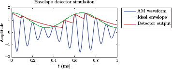
MATLAB graph for envelope detector simulation with fc = 10 kHz, fm = 1.5 kHz,μ = 0.6, and τ = 0.3 ms.
Observe how the envelope detector loses track of the envelope as a result of a time constant that is too large.
Software resources:
matex_11_8a.m
matex_11_8b.m
Problems
11.1. Consider the single-tone modulated AM signal xAM (t) given by Eqn. (11.07). For each set of parameters listed below, determine the missing parameter value.
- Am = 2, μ = 0.7, Ac = ?
- Am = 3, μ = 0.85, Ac = ?
- Ac = 2, μ = 0.9, Am = ?
- Ac = 3, Am = 2.5, μ = ?
11.2. Manually sketch each single-tone modulated AM signal, the parameters of which are given below. Indicate critical values on each axis.
- Ac = 3, μ = 0.6, fc = 10 Hz, fm = 2 Hz
- Ac = 3, μ = 1.3, fc = 10 Hz, fm = 2 Hz
- Ac = 5, Am = 4, fc = 25 Hz, fm = 8 Hz
11.3. A sinusoidal carrier is in the form
For each modulating signal listed below, the modulation index is required to be μ = 0.7. Determine the parameter Ac in each case.
- m (t)= cos(4πt) + 2 cos(6πt)
- m (t)= cos(4πt) + 3 sin(6πt)
- m (t)= 3 sin(4πt) + 2 cos(6πt − π/3)
11.4. Refer to the tone-modulated AM signals, the parameters of which are listed below. For each, draw the phasors Xcar, and at the time instant indicated.
- Ac = 3, μ = 0.6, fc = 10 Hz, fm = 2 Hz, t = 0.35 s
- Ac = 3, μ = 1.3, fc = 10 Hz, fm = 2 Hz, t = 0.6 s
- Ac = 5, Am = 4, fc = 25 Hz, fm = 8 Hz, t = 150 ms
11.5. Refer to the tone-modulated AM signals the parameters of which are listed in Problem 11.1. Compute and graph the frequency spectrum of each signal.
11.6. Refer to Problem 11.3. For each modulating signal determine and sketch the frequency spectrum of xAM (t). Afterwards determine the modulation efficiency η. (Use the value of Ac computed in Problem 11.2 for each case.)
11.7. The frequency spectrum M (f) of a message signal m (t) is shown in Fig. P.11.7.
The signal m (t) is used as input to the AM modulator shown in Fig. 11.14. The carrier amplitude is Ac = 1.5 and the carrier frequency is fc = 10 kHz. Sketch the frequency spectrum of the signal xAM (t).
11.8. Refer to the message signal m (t) the spectrum of which is shown in Fig. P.11.7. Assume that this signal is used as input to the AM modulator shown in Fig. 11.20. The carrier amplitude is Bc = 1.5 and the carrier frequency is fc = 10 kHz. The nonlinear device has the input-output characteristic
- Determine and sketch the frequency spectrum of the signal at the output of the nonlinear device.
- Specify the appropriate bandpass filter to produce the AM signal xAM (t).
11.9. A single-tone modulated signal is shown in Fig. P.11.9.
Estimate the following from the figure:
- Carrier frequency fc
- Single-tone message frequency fm
- Modulation index
- Efficiency of modulation
11.10. Refer to Problem 11.3. For each modulating signal determine the efficiency of modulation using the value of Ac computed in Problem 11.3.
11.11. Consider the switching modulator shown in Fig. 11.15. Let the message signal be the single tone
The carrier amplitude is Bc = 5, and the carrier frequency is fc = 800 Hz.
- Sketch the signal vin (t).
- Assuming the diode is ideal, sketch the signal vout (t).
- Determine the magnitude characteristic of an ideal bandpass filter that would be appropriate for use in this switching modulator.
11.12. Consider the balanced modulator block diagram shown in Fig. P.11.12 which can be used for producing DSB with suppressed carrier without the need for filtering.
Determine the intermediate signals w1 (t) and w2 (t). Show that the output signal is the proper DSB-modulated signal with the carrier suppressed.
11.13. Refer to the message signal m (t) the frequency spectrum M (f) of which is shown in Fig. P.11.7. A sinusoidal carrier with amplitude Ac = 1.5 and the carrier frequency fc = 10 kHz is to be used in conjunction with this signal.
- If the signal m (t) is used for modulating a sinusoidal carrier using DSB, sketch the frequency spectrum of the signal xDSB (t).
- Repeat part (a) using SSB with the upper sideband retained.
- Repeat part (a) using SSB with the lower sideband retained.
11.14. A single-tone modulated AM signal given by
is applied to the envelope detector shown in Fig. 11.21. Determine an appropriate time constant for the envelope detector so that the single-tone message signal is recovered correctly. Based on the time constant found, pick practical values for R and C.
11.15. Refer to the coherent demodulator shown in Fig. P.11.15. Assume that the local oscillator signal is not perfectly synchronized with the original carrier, but rather has a phase error θ as shown.
Determine the signal r (t) and the bandpass filter output . Explain the effect of the phase error on these signals.
11.16. Refer to the coherent demodulator shown in Fig. P.11.16. Assume that the local oscillator signal is not perfectly synchronized with the original carrier, but rather has a frequency error so that the local carrier frequency is fc + Δf.
Determine the signal r (t) and the bandpass filter output . Explain the effect of the frequency error on these signals.

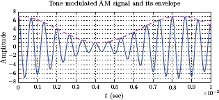
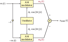


MATLAB Problems
11.17. Refer to Problem 11.2. For each set of parameters given, develop a MATLAB script to compute and graph the corresponding AM signal. In each case choose an appropriate sampling interval and produce a graph that spans at least three periods of the modulating tone.
11.18. Refer to Problem 11.3. For each modulating signal write a script to compute and graph xAM (t). Choose the sampling interval appropriately, and graph the corresponding signal in a time interval sufficient to show relevant details.
11.19. Refer to Problem 11.3. Determine the fundamental frequency and the fundamental period for each multi-tone-modulated AM signal. Write a script for each case to produce 1024 samples of exactly one period. Compute and graph the approximate EFS spectrum using the function ss_efsapprox(..).
11.20. Refer to Problem 11.11. Write a MATLAB script to
- Compute and graph the signal vin (t).
- Compute and sketch the signal vout (t) assuming that the diode is ideal.
- Use the function ss_switchmod(..) developed in MATLAB Exercise 11.3 to compute the output signal xAM (t). Graph the result.
11.21. Using the ss_switchmod(..) as the starting point, develop a new MATLAB function ss_switchmod2(..) to simulate a switching modulator that uses the more realistic diode model shown in Fig. P.11.21 instead of the ideal diode model.
Afterwards rework Problem 11.20 using the function ss_switchmod2(..) instead of ss_switchmod(..). Compare the results.
11.22. Refer to Problem 11.14. Write a MATLAB script to generate samples of the signal xAM (t) and then to simulate the envelope detector using the function ss_envdet(..) developed in MATLAB Exercise 11.7. First, use the value of τ found in Problem 11.14. Afterwards repeat with half the value found and with twice the value found. Graph the envelope detector output signal for each case and compare the results.
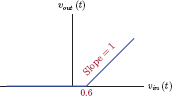
MATLAB Projects
11.23. A mystery AM signal has been saved into the data file “ch11data.mat”. It can be loaded into MATLAB workspace with the statement
>> load ch11data. matcreating two vectors named “t” and “xAM” in the workspace.
- Graph the signal xAM (t).
- Determine the sampling rate used in creating the vector “xAM” by inspecting the elements of the vector “t”. Compute the FFT of the signal, and graph the spectrum using actual frequencies in Hz based on the sampling rate used.
- Inspect the spectrum graph obtained in part (b). What seems to be the carrier frequency? How many tones are in the modulating signal m (t), and what are their frequencies?
- Using function cheby1(..) design a Chebyshev type-I band-reject filter to remove the carrier frequency. Adjust the passband cutoff frequencies so that the sideband frequencies are kept and the carrier frequency is removed. A ninth-order filter with a passband ripple of 0.5 dB may be an appropriate starting point. Compute and graph the magnitude response of the designed filter using the function freqz(..) Adjust design parameters and repeat the design as necessary.
- Use the function filter(..) to apply the AM signal to the Chebyshev type-I filter designed in part (d). Create a vector “x2” with the samples of the Chebyshev filter output signal. Graph the output signal.
- Compute and graph the frequency spectrum of the output signal using the FFT. Is the carrier frequency gone?
- Estimate the power in the original AM signal and in the signal at the output of the Chebyshev band-reject filter. (Hint: Scalar product operator can be used in MATLAB with some scaling afterwards to estimate the power in a signal.) Using these two power estimates, compute an estimate of modulation efficiency.
-
Develop a MATLAB function ss_coherent(..) to simulate the coherent demodulator shown in Fig. 11.24. The syntax of the function should be as follows:
>> mhat = ss_coherent (xAM,Ts,fc,theta,deltaf)The input arguments to the function are
xAM:
Vector holding samples of the AM signal.
Ts:
Sampling intetrval used for signal in vector “xAM”.
fc:
Carrier frequency in Hz.
theta:
Phase error of the local carrier (in radians).
deltaf:
Frequency error of the local carrier (in Hz).
The vector “mhat” holds samples of the output signal. Internally, implement the bandpass filter as the cascade of two filters: A fifth-order Butterworth lowpass filter with the appropriate cutoff frequency, and a sixth-order Chebyshev type-I highpass filter to remove frequencies less than 2 percent of the carrier frequency.
Test the function ss_coherent(..) with the signal
using a sampling rate of fs = 25 kHz. Set phase and frequency errors equal to zero. Generate samples of the AM signal for t = 0,..., 100 ms. Compute and graph the simulated output signal .
- Repeat part (b) using a phase error of θ = π/10 radians.
- Repeat part (b) using a frequency error of Δf = 60 Hz.
11.25. A SSB-modulated signal with lower sideband retained was given by Eqn. (11.100) and is repeated here:
The term represents the Hilbert transform of m (t)
Using the fdatool program in MATLAB, design a length-55 FIR filter to approximate an ideal Hilbert transform filter. Export the impulse response of the designed filter to a data file.
-
and use the carrier frequency fc = 1000 Hz. Write a script to compute the signal xSSB,L (t) as given above. Your script should
- Load the length-55 Hilbert transform filter impulse from data file.
- Generate samples of m (t) usingasamplingrateof fc = 25 kHz.
- Process m (t) through the FIR filter designed to obtain an approximation to the Hilbert transform .
- Compute an approximation to xSSB,L (t) as specified. Hint: Keep in mind that the length-55 FIR filter has a delay of (55 − 1)/2 = 27 samples, so it produces an approximation to a delayed version of .
1 This is actually an oversimplification. In an actual communication channel, the signal is not necessarily distorted first and contaminated by noise afterwards; distortion and contamination take place simultaneously in a distributed fashion, resulting in a much more difficult model for analysis.
2 cos (a) cos(b) = ½ cos (a + b)+ ½ cos (a − b).
3 sin (a) = cos(a − π/2).
4 cos 2 (a) = ½ [1 + cos (2a)].