
Laplace Transform for Continuous-Time Signals and Systems
Chapter Objectives
- Learn the Laplace transform as a more generalized version of the Fourier transform studied in Chapter 4.
- Understand the convergence characteristics of the Laplace transform and the concept of region of convergence.
- Explore the properties of the Laplace transform.
- Understand the use of the Laplace transform for modeling CTLTI systems. Learn the s-domain system function and its use for solving signal-system interaction problems.
- Learn techniques for obtaining simulation diagrams for CTLTI systems based on the s-domain system function.
- Learn the use of the unilateral Laplace transform for solving differential equations with specified initial conditions.
7.1 Introduction
In earlier chapters we have studied Fourier analysis techniques for understanding characteristics of continuous-time signals and systems. Chapter 4 focused on representing continuous-time signals in the frequency domain through the use of Fourier series and Fourier transform. We have also adapted frequency domain analysis techniques for use with linear and time-invariant systems in the form of a system function.
Some limitations exist in the use of Fourier series and Fourier transform for analyzing signals and systems. A signal must be absolute integrable to have a representation based on Fourier series or Fourier transform. Consider, for example, a ramp signal in the form x (t) = tu (t). Such a signal cannot be analyzed using the Fourier transform since it is not absolute integrable. Similarly, a system function based on the Fourier transform is only available for systems for which the impulse response is absolute integrable. Consequently, Fourier transform techniques are usable only with stable systems.
Laplace transform, named after the French mathematician Pierre Simon Laplace (1749-1827), overcomes these limitations. It can be seen as an extension, or a generalization, of the Fourier transform. In contrast, the Fourier transform is a special case, or a limited view, of the Laplace transform. A signal that does not have a Fourier transform may still have a Laplace transform for a certain range of the transform variable. Similarly, an unstable system that does not have a system function based on the Fourier transform may still have a system function based on the Laplace transform.
The Fourier transform of a signal, if it exists, can be obtained from its Laplace transform while the reverse is not generally true. In addition to analysis of signals and systems, block diagram and signal flow graph structures for simulating continuous-time systems can be developed using Laplace transform techniques. The unilateral variant of the Laplace transform can be used for solving differential equations subject to specified initial conditions.
We begin with the basic definition of the Laplace transform and its application to some simple signals. The significance of the issue of convergence of the Laplace transform will become apparent throughout this discussion. Section 7.2 is dedicated to the convergence properties of the Laplace transform, and to the concept of region of convergence. We cover the fundamental properties of the Laplace transform in Section 7.3. These properties will prove useful in working with the Laplace transform for analyzing signals and systems, for understanding system characteristics, and for working with signal-system interaction problems. Proofs of significant Laplace transform properties are given not just for the sake of providing proofs, but also to provide further insight and experience on working with transforms. Techniques for computing the inverse Laplace transform are presented in Section 7.4. Use of the Laplace transform for the analysis of linear and time-invariant systems is discussed in Section 7.5, and the s-domain system function concept is introduced. Derivations of block diagram structures for the simulation of continuous-time systems based on the s-domain system function are covered in Section 7.6. In Section 7.7 the unilateral variant of the Laplace transform is introduced, and it is shown that it is useful in solving differential equations with specified initial conditions.
The Laplace transform of a continuous-time signal x (t) is defined as
where s, the independent variable of the transform, is a complex variable.
Notationally, the relationship between the signal x (t) and the transform X (s) can be expressed in the form
or in the form
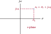
Since the parameter s is a complex variable, we will represent it graphically as a point in the complex s-plane. It is customary to draw the s-plane with σ as its real axis and ω as its imaginary axis. Based on this convention the complex variable s is written in Cartesian form as
A specific value s1 = σ1 + jω1 of the variable s can be shown as a point in the s-plane as illustrated in Fig. 7.1 with σ1 equal to the horizontal displacement of the point from the origin and ω1 as the vertical displacement from the origin. If the Laplace transform converges at the point s = s1, its value can be computed by evaluating the integral in Eqn. (7.1) at that point.
Using the Cartesian form of the variable s given by Eqn. (7.4), the transform of the signal x(t) becomes
At this point it would be interesting to let the value of σ, the real part of s, be fixed at σ = σ1. Thus, we have s = σ1 + jω. If the imaginary part ω is allowed to vary in the range −∞ < ω < ∞, the trajectory of the points s in the complex plane would be a vertical line with a horizontal displacement of σ1 from the origin, that is, a vertical line that passes through the point s = σ1 + j0. This is illustrated in Fig. 7.2.

If the transform in Eqn. (7.5) is evaluated at points on the vertical line represented by the trajectory s = σ1 + jω, we get
Comparison of the result in Eqn. (7.6) with the definition of the Fourier transform in Eqn. (4.127) in Chapter 4 suggests that the Laplace transform X (s) evaluated on the trajectory s = σ1 + ω is identical to the Fourier transform of the signal .
This important conclusion can be summarized as follows:
In the s-plane consider a vertical line passing through the point s = σ1 for a fixed value of σ1. The Laplace transform of a signal x (t) evaluated on this line as the parameter ω is varied from ω = −∞ to ω = ∞ is the same as the Fourier transform of the signal .
If we choose σ1 = 0 then the vertical line in Fig. 7.2 coincides with the jω axis of the s-plane, and the Laplace transform evaluated on that trajectory becomes
Consider the Laplace transform of a signal x (t) evaluated at all points on the jω axis of the s-plane as ω is varied from ω = −∞ to ω = ∞. The result is the same as the Fourier transform X (ω) of the signal.
An easy way to visualize the relationship between the Laplace transform and the Fourier transform is the following: Imagine that the Laplace transform evaluated at every point in the s-plane results in a three-dimensional surface. The transform X (s) is complex-valued in general; therefore, it may be difficult to visualize it as a surface unless we are willing to accept the notion of a complex-valued surface. Alternatively, we may split the complex function X (s) into its magnitude and phase, each defining a surface. In any case, if we were to take the surface represented by the Laplace transform and cut it the through the length of the jω axis, the profile of the cross-section would be the same as the Fourier transform of the signal. This relationship is illustrated graphically in Fig. 7.3.
Consider a particular transform in the form
which is complex-valued. We will choose to graph only its magnitude |X (s)| as a three-dimensional surface which is shown in Fig. 7.3(a). Also shown in the figure is the set of values of |X (s)| computed at points on the jω axis of the s-plane. In Fig. 7.3(b) the magnitude of the Fourier transform X (ω) of the same signal is graphed as a function of the radian frequency ω. Notice how the jω axis of the s-plane becomes the frequency axis for the Fourier transform.
For the same transform under consideration, Fig. 7.4 shows the values on the trajectory s = 0.5 + jω. Recall that the values of |X (s)| on this trajectory are the same as the magnitude of the Fourier transform of the modified signal [x (t)e−0.5t].
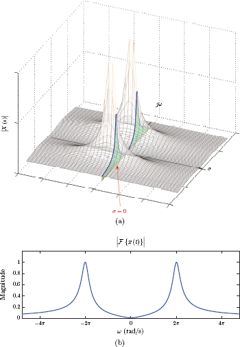
(a) The magnitude |X (s)| shown as a surface plot along with the the magnitude computed on the jω axis of the s-plane, (b) the magnitude of the Fourier transform as a function of ω.
The Laplace transform as defined by Eqn. (7.1) is referred to as the bilateral (two-sided) Laplace transform. A variant of the Laplace transform known as the unilateral (one-sided) Laplace transform will be introduced in Section 7.7 as an alternative analysis tool. In this text, when we refer to Laplace transform without the qualifier word “bilateral” or “unilateral”, we will always imply the more general bilateral Laplace transform as defined in Eqn. (7.1).
Interactive Demo: lap_demol.m
The demo program “lap_demo1.m” is based on the Laplace transform given by Eqn. (7.8). The magnitude of the transform in question is shown in Fig. 7.3(a). The demo program computes this magnitude and graphs it as a three-dimensional mesh. It can be rotated freely for viewing from any angle by using the rotation tool in the toolbar. The magnitude of the transform is also evaluated on the vertical line s = σ1 + jω in the s-plane, and displayed as a two-dimensional graph. The value σ1 may be varied through the use of a slider control.
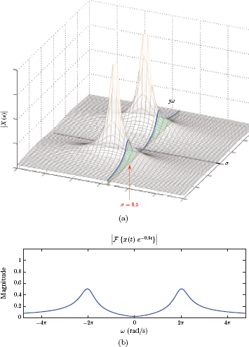
(a) The magnitude |X (s)| shown as a surface plot along with the the magnitude computed on the trajectory s = 0.5 + jω on the s-plane, (b) the magnitude of the Fourier transform of x (t) e−0.5t.
Software resources:
lap_demol.m
Software resources: |
See MATLAB Exercises 7.1 and 7.2. |
Example 7.1: Laplace transform of the unit impulse
Find the Laplace transform of the unit-impulse signal
Solution: Applying the definition of the Laplace transform given by Eqn. (7.1) we get
using the sifting property of the unit-impulse function. Therefore, the Laplace transform of the unit-impulse signal is constant and equal to unity. Since it does not depend on the value of s, it converges at every point in the s-plane with no exceptions.
Example 7.2: Laplace Transform of a time-shifted unit impulse
Find the Laplace transform of the time-shifted unit-impulse signal
Solution: Applying the Laplace transform definition we obtain
Again we have used the sifting property of the unit-impulse function. If s = σ + jω, then Eqn. (7.10) becomes
The transform obtained in Eqn. (7.10) converges as long as σ = Re {s} > −∞.
Example 7.3: Laplace transform of the unit-step signal
Find the Laplace transform of the unit-step signal
Solution: Substituting x (t) = u (t) into the Laplace transform definition we obtain
Since u (t) = 1 for t > 0 and u (t) = 0 for t < 0, the lower limit of the integral can be changed to t = 0 and the unit-step term can be dropped to yield
To evaluate the integral of Eqn. (7.11) for the specified limits we will use the Cartesian form of the complex variable s. Substituting s = σ + jω
It is obvious that, for the exponential term eσt to converge as t → ∞, we need σ > 0:
The transform expression found in Eqn. (7.12) is valid only for points in the right half of the s-plane. This region is shown shaded in Fig. 7.5. Note that the transform does not converge at points on the jω axis. It converges at any point to the right of the jω axis regardless of how close to the axis it might be.

Example 7.4: Laplace transform of a time-shifted unit-step signal
Find the Laplace transform of the time-shifted unit-step signal
Solution: Using x (t) = u (t − τ) in the Laplace transform definition we get
Since u (t − τ) = 1 for t > τ and u (t − τ) = 0 for t < τ, the lower limit of the integral can be changed to t = τ and the unit-step function can be dropped without affecting the result.
As in Example 7.3, the integral can be evaluated only for σ = Re {s} > 0, and its value is
Convergence conditions for the the transform of u (t − τ) are the same as those found in Example 7.3 for the transform of u (t).
We observe from the last two examples that, when we find the Laplace transform X (s) of a signal, we also need to specify the region in which the transform is valid. The collection of all points in the s-plane for which the Laplace transform converges is called the region of convergence (ROC).
Recall that in Eqn. (7.7) we have represented the Laplace transform of a signal x (t) as equivalent to the Fourier transform of the modified signal [x (t) e−σt]. Consequently, the conditions for the convergence of the Laplace transform of x (t) are identical to the conditions for the convergence of the Fourier transform of [x (t) e−σt]. Using Dirichlet conditions for the latter, we need the signal [x (t) e−σt] to be absolute integrable for the transform to exist, that is,
The convergence condition stated in Eqn. (7.14) highlights the versatility of the Laplace transform over the Fourier transform. The Fourier transform of a signal x (t) exists is the signal is absolute integrable, and does not exist otherwise. Therefore, the existence of the Fourier transform is a binary question; the answer to it is either yes or no. In contrast, if the signal x (t) is not absolute integrable, we may still be able to find values of σ for which the modified signal [x (t) e−σt] is absolute integrable. Therefore, the Laplace transform of the signal x (t) may exist for some values of σ. The question of existence for the Laplace transform is not a binary one; it is a question of which values of σ allow the transform to converge.
The next two examples will further highlight the significance of the region of convergence for the Laplace transform. The fundamental characteristics of the region of convergence will be discussed in detail in Section 7.2.
Example 7.5: Laplace transform of a causal exponential signal
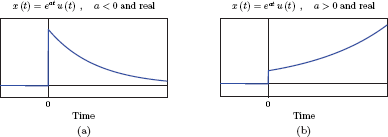
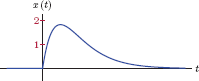
Find the Laplace transform of the signal
where a is any real or complex constant.
Solution: The signal x (t) is causal since x (t) = 0 for t < 0. Applying the Laplace transform definition to x (t) results in
Changing the lower limit of the integral to t = 0 and dropping the factor u (t) we get
The parameter a may be real or complex-valued. Let us assume that it is in the form a = ar + jai to keep the results general. For the purpose of evaluating the integral in Eqn. (7.15) we will substitute s = σ + jω and write the transform as
For the result of Eqn. (7.16) to converge at the upper limit, we need
which establishes the ROC for the transform. With the condition in Eqn. (7.17) satisfied, the exponential term in Eqn. (7.16) becomes zero as t → ∞, and we obtain
The ROC is the region to the right of the vertical line that goes through the point s = ar + jai as shown in Fig. 7.6.

It is interesting to look at the shape of the signal x (t) in conjunction with the ROC.
- Fig. 7.7 shows the signal for the case where a is real-valued. The signal x (t) is a decaying exponential for a < 0, and a growing exponential for a > 0.
- Real and imaginary parts of the signal x (t) are shown in Figs. 7.8 and 7.9 for the case of parameter a being complex-valued. Fig. 7.8 illustrates the possibility of Re {a} < 0. Real and imaginary parts of x (t) exhibit oscillatory behavior with exponential damping. In contrast, if Re {a} > 0, both real and imaginary parts of x (t) grow exponentially as shown in Fig. 7.9.
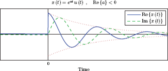

Since the ROC is to the right of a vertical line, for the case Re {a} < 0 the jω axis is part of the ROC whereas, for the case Re {a} > 0, it is not.
Recall from the previous discussion that the Fourier transform of the signal x (t) is equal to the Laplace transform evaluated on the jω axis of the s-plane. Consequently, the Fourier transform of the signal exists only if the region of convergence includes the jω axis. We conclude that, for the Fourier transform of the signal x (t) to exist, we need Re {a} < 0. Signals in Figs. 7.7(a) and 7.8 have Fourier transforms whereas signals in Figs. 7.7(b) and 7.9 do not. This is consistent with the existence conditions discussed in Chapter 4.
Software resources:
ex_7_5a.m
ex_7_5b. m
Example 7.6: Laplace transform of an anti-causal exponential signal
Find the Laplace transform of the signal
where a is any real or complex constant.
Solution: In this case the signal x (t) is anti-causal since it is equal to zero for t > 0. Substituting x (t) into the Laplace transform definition we get
Since u (−t) = 1 for t < 0 and u (−t) = 0 for t > 0, changing the upper limit of the integral to t = 0 and dropping the factor u (−t) would have no effect on the result. Therefore
The parameter a may be real or complex valued. We will assume that it is in the general form a = ar + jai. For the purpose of evaluating the integral in Eqn. (7.19) let us substitute s = σ + jω and write the transform as
In contrast with Example 7.5, the critical end of the integral with respect to convergence is its lower limit. To evaluate the result of Eqn. (7.20) at the lower limit, we need
or equivalently
which establishes the ROC for the transform. With the condition in Eqn. (7.21) satisfied, the exponential term in Eqn. (7.20) becomes zero as t → −∞, and we obtain
The ROC is the region to the left of the vertical line that goes through the point s = ar + jai as shown in Fig. 7.10.

As in Example 7.5 we will look at the shape of the signal x (t) in conjunction with the ROC.
Fig. 7.11 shows the signal for the case where a is real-valued. For a < 0, the signal grows exponentially as t → −∞. In contrast, for a > 0 the signal decays exponentially.
For complex a, real and imaginary parts of x (t) exhibit oscillatory behavior. For Re {a} < 0 the signal grows exponentially as shown in Fig. 7.12. In contrast, oscillations are damped exponentially for Re {a} > 0. This is shown in Fig. 7.13.
x (t) = —eat u (—t) , a < 0 and real x (t) = —eat u (—t) , a > 0 and real

The signal x (t) of Example 7.6 for the real-valued parameter a and (a) a < 0 and (b) a > 0.
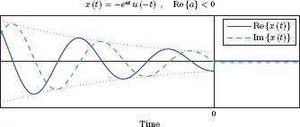
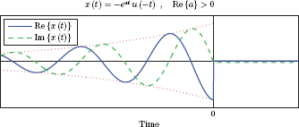
For the case Re {a} > 0 the jω axis of the s-plane is part of the ROC. For the case Re {a} < 0, however, it is not. Thus, the Fourier transform of the signal x (t) exists only when Re {a} > 0.
Software resources:
ex_7_6a.m
ex_7_6b.m
Examples 7.5 and 7.6 demonstrate a fundamental concept for the Laplace transform: It is possible for two different signals to have the same transform expression for X (s). In both of the examples above we have found the transform
What separates the two results apart is the ROC. In order for us to uniquely identify which signal among the two led to a particular transform, the ROC must be specified along with the transform. The following two transform pairs will be fundamental in determining to which signal a given transform corresponds:
Sometimes we need to solve the inverse problem of finding the signal x (t) with a given Laplace transform X (s). Given a transform
we need to know the ROC to determine if the signal x (t) is the one in Eqn. (7.22) or the one in Eqn. (7.23). This will be very important when we work with inverse Laplace transform in Section 7.4 later in this chapter. In order to avoid ambiguity, we will adopt the convention that the ROC is an integral part of the Laplace transform. It must be specified explicitly, or implied by means of another property of the signal or the system under consideration every time a transform is given.
In each of the Examples 7.3, 7.5 and 7.6 we have obtained the Laplace transform of the specified signal in the form of a rational function of s, that is, a ratio of two polynomials in s. In the general case, a rational transform X (s) is expressed in the form
where the numerator B (s) and the denominator A (s) are polynomials of s. Let the numerator polynomial be written in factored form as
where z1, z2,..., zM are its roots. Similarly, let p1, p2,..., pN be the roots of the denominator polynomial so that
The transform can be written as
In Eqns. (7.26) and (7.27) the parameters M and N are the numerator order and the denominator order respectively. The larger of M and N is the order of the transform X (s). The roots of the numerator polynomial are referred to as the zeros of X (s). In contrast, the roots of the denominator polynomial are the poles of X (s). The transform does not converge at a pole; therefore, the ROC cannot contain any poles. In the next section we will see that the poles of the transform also determine the boundaries of the ROC.
Software resources: |
See MATLAB Exercises 7.3. |
Example 7.7: Laplace transform of a pulse signal
Determine the Laplace transform of the pulse signal
which is shown in Fig. 7.14.

Solution: The Laplace transform of the signal x (t) is computed as
At a first glance we may be tempted to think that the transform X (s) might not converge at s = 0 since the denominator of X (s) becomes equal to zero at s = 0. We must realize, however, that the numerator of X (s) is also equal to zero at s = 0. Using L’Hospital’s rule on X (s) we obtain its value at s = 0 as
confirming the fact that X (s) does indeed converge at s = 0. As a matter of fact, X (s) converges everywhere on the s-plane with the exception of s = −∞±jω. In order to observe this, let us write the Taylor series representation of the exponential term e−sτ:
The numerator of X (s) can be written as
and the transform X (s) can be written in series form
Thus, the transform X (s) has an infinite number of zeros and no finite poles. Its ROC is
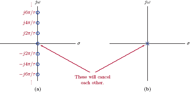
It will be interesting to determine the zeros of the transform. The roots of the numerator are found by solving the equation
The value S = 0 is a solution for Eqn. (7.29), however, there must be other solutions as well. Realizing that ej2πk = 1 for all integer values of k, Eqn. (7.29) can be written as
which leads to the set of solutions
The numerator of X (s) has an infinite number of roots, all on the jω-axis of the s-plane. The roots are uniformly spaced, and occur at integer multiples of j2π/τ. The denominator polynomial of X (s) is just equal to s, and has only one root at s = 0. This single root of the denominator cancels the root of the numerator at s = 0, so that there is neither a zero nor a pole at the origin of the s-plane. We are left with zeros at
Numerator and denominator roots are shown in Fig. 7.15. The pole-zero diagram for X (s) is shown in Fig. 7.16.

To get a sense of what the transform looks like in the s-plane, we will compute and graph the magnitude |X (s)| of the transform as a three-dimensional surface (recall that the transform X (s) is complex-valued, so we can only graph part of it as a surface, that is, we can graph magnitude, phase, real part or imaginary part). Let s = σ + jω, and write the transform as
The squared magnitude of a complex function is computed by multiplying it with its own complex conjugate; therefore
and the magnitude of the transform is
which is shown in Fig. 7.17(a) as a surface graph. Note how the zeros equally spaced on the jω-axis cause the magnitude surface to dip down. In addition to the surface graph, magnitude values computed at points on the jω-axis of the s-plane are marked on the surface in Fig. 7.17(a). For comparison, the magnitude of the Fourier transform of the signal x (t) computed for the range of angular frequency values −10π/τ < ω < 10π/τ is shown in Fig. 7.17(b). It should be compared to the values marked on the surface graph that correspond to the magnitude of the Laplace transform evaluated on the jω-axis.

(a) The magnitude |X (s)| for Example 7.7 shown as a surface plot along with the jω-axis of the s-plane and the magnitude of the transform computed on that axis, (b) the magnitude of the Fourier transform of x (t) as a function of ω.
ex_7_7a.m
ex_7_7b.m
Interactive Demo: lap_demo2.m
The demo program “lap_demo2.m” is based on the Laplace transform of the pulse signal analyzed in Example 7.7. The magnitude of the transform in question was shown in Fig. 7.17(a). The demo program computes this magnitude and graphs it as a three-dimensional mesh. It can be rotated freely for viewing from any angle by using the rotation tool in the toolbar. The magnitude of the transform is also evaluated on the vertical line s = σ1 + jω in the s-plane, and displayed as a two-dimensional graph. This corresponds to the Fourier transform of the modified signal . The value σ1 and the pulse width τ may be varied through the use of slider controls.
lap_demo2.m
Example 7.8: Laplace Transform of complex exponential signal
Find the Laplace transform of the signal
The parameter ω0 is real and positive, and is in radians.
Solution: Applying the Laplace transform definition directly to the signal x (t) leads to
Since x (t) is causal, the lower limit of the summation can be set to t = 0, and the u (t) term can be dropped to yield
The upper limit is critical in Eqn. (7.32). To be able to evaluate the expression at s → ∞ we need
and therefore
Provided that this condition is satisfied, the transform in Eqn. (7.32) is computed as
The transform X (s) has one pole at s = jω0, and its ROC is the region to the right of the vertical line that passes through its pole. This is illustrated in Fig. 7.18.

7.2 Characteristics of the Region of Convergence
Through the examples we have worked on so far, we have observed that the Laplace transform of a continuous-time signal always needs to be considered in conjunction with its region of convergence, that is, the region in the s-plane in which the transform converges. In this section we will summarize and justify the fundamental characteristics of the region of convergence.
For a finite-duration signal the ROC is the entire s-plane provided that the signal is absolute integrable. The extreme points such as Re {s} → ±∞ need to be checked separately.
Let the signal x (t) be equal to zero outside the interval t1 < t < t2. The Laplace transform is
If the signal x (t) is absolute integrable, then the transform given by Eqn. (7.33) converges on the vertical line s = jω. Since the limits of the integral are finite, it also converges for all other values of s.
2. For a general signal the ROC is in the form of a vertical strip. It is either to the right of a vertical line, to the left of a vertical line, or between two vertical lines as shown in Fig. 7.19.
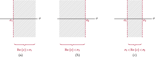
This property is easy to justify. We have established in Eqn. (7.7) of the previous section that, for s = σ + jω, the values of the Laplace transform of the signal x (t) are identical to the values of the Fourier transform of the signal x (t) e−σt. Therefore, the convergence of the Laplace transform for s = σ + jω is equivalent to the convergence of the Fourier transform of the signal x (t) e−σt, and it requires that
Thus, the ROC depends only on σ and not on ω, explaining why the region is in the form of a vertical strip. Following are the possibilities for the ROC:
3. For a rational transform X (s) the ROC cannot contain any poles.
By definition, poles of X (s) are values of s that make the transform infinitely large. For rational Laplace transforms, poles are the roots of the denominator polynomial. Since the transform does not converge at a pole, the ROC must naturally exclude all poles of the transform.
4. The ROC for the Laplace transform of a causal signal is the region to the right of a vertical line, and is expressed as
Since a causal signal equals zero for all t < 0, its Laplace transform can be written as
Using s = σ + jω and remembering that the convergence of the Laplace transform is equivalent to the signal x (t) e−σt being absolute integrable leads to the convergence condition
If we can find a value of σ for which Eqn. (7.35) is satisfied, then any larger value of σ will satisfy Eqn. (7.35) as well. All we need to do is find the value σ = σ1 for the boundary, and the ROC will be the region to the right of the vertical line that passes through the point s = σ1.
5. The ROC for the Laplace transform of an anti-causal signal is the region to the left of a vertical line, and is expressed as
The justification of this property will be similar to that of the previous one. Since an anti-causal signal is equal to zero for all t > 0, its Laplace transform can be written as
Using s = σ + jω the condition for the convergence of the Laplace transform can be expressed through the equivalent condition for the absolute integrability of the signal x (t) e−σt as
If we can find a value of σ for which Eqn. (7.36) is satisfied, then any smaller value of σ will satisfy Eqn. (7.36) as well. Once a value σ = σ2 is found for the boundary, the ROC will be the region to the left of the vertical line that passes through the point s = σ2.
6. The ROC for the Laplace transform of a signal that is neither causal nor anti-causal is a strip between two vertical lines, and can be expressed as
Any signal x (t) can be written as the sum of a causal signal and an anti-causal signal. Let the two signals xR (t) and xL (t) be defined in terms of the signal x (t) as
and
so that xR (t) is causal, xL (t) is anti-causal, and
Let the Laplace transforms of these two signals be
The Laplace transform of the signal x (t) is
The ROC for X (s) is at least the overlap of the two regions, that is,
provided that σ2 > σ1 (otherwise there may be no overlap, and the Laplace transform may not exist at any point in the s-plane).
In some cases the ROC may actually be larger than the overlap in Eqn. (7.38) if the addition of the two transforms in Eqn. (7.37) results in the cancellation of a pole that sets one of the boundaries.
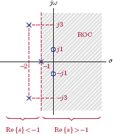
Example 7.9: Laplace transform of two-sided exponential signal
Find the Laplace transform of the signal
Solution: The specified signal exists for all t, and can be written as
Thus, x (t) is the sum of a causal signal xR (t) and an anti-causal signal xL (t):
Two components of x (t) are
When we discuss the properties of the Laplace transform later in Section 7.3 we will show that the Laplace transform is linear. Consequently, the transform of the sum of two signals is equal to the sum of their respective transforms, and X (s) can be written as
The individual transforms that make up X (s) in Eqn. (7.39) can be determined by adapting the results obtained earlier in Eqns. (7.22) and (7.23) as:
The ROC for XR (s) and XL (s) are shown in Fig. 7.20.

The transform X (s) can be computed as
X (s) has a two poles at s = ±1. For this transform to converge both XR (s) and XL (s) must converge. Therefore, the ROC for X (s) is the overlap of the ROCs of XR (s) and XL (s)
and is shown in Fig. 7.21.

Software resources:
ex_7_9.m
7.3 Properties of the Laplace Transform
The important properties of the Laplace transform will be summarized in this section, and the proof of each will be given. The use of these properties greatly simplifies the application of the Laplace transform to problems involving the analysis of continuous-time signals and systems.
7.3.1 Linearity
Laplace transform is linear. For any two transforms x1 (t) and x2 (t) with their respective transforms
and any two constants α1 and α2, it can be shown that the following relationship holds:
Linearity of the Laplace transform:
Proof: The proof is straightforward using the Laplace transform definition given by Eqn. (7.1). Substituting x (t) = α1x1 (t) + α2x2 (t) into Eqn. (7.1) we get
The integral in Eqn. (7.43) can be separated into two integrals as
The Laplace transform of a weighted sum of two signals is equal to the same weighted sum of their respective transforms X1 (s) and X2 (s). The ROC for the resulting transform is at least the overlap of the two individual transforms, if such an overlap exists. The ROC may be greater than the overlap of the two regions if the addition of the two transforms results in the cancellation of a pole.
The linearity property proven above for two signals can be generalized to any arbitrary number of signals. The Laplace transform of a weighted sum of any number of signals is equal to the same weighted sum of their respective transforms.
Example 7.10: Using the linearity property of the Laplace transform
Determine the Laplace transform of the signal
Solution: A general expression for the Laplace transform of the causal exponential signal was found in Example 7.5 as
Applying this result to the exponential terms in x (t) we get
and
Combining the results in Eqns. (7.45) and (7.46) and using the linearity property we arrive at the desired result:
The ROC for X (s) is the overlap of the two regions in Eqns. (7.45) and (7.46), namely
Fig. 7.22 illustrates the poles and the ROCs of the individual terms X1 (s) and X2 (s) as well as the ROC of the transform X (s) obtained as the overlap of the two.
Example 7.11: Laplace transform of a cosine signal
Find the Laplace transform of the signal
Solution: Using Euler’s formula for the cos (ω0t) term, the signal x (t) can be written as
and its Laplace transform is
Using the linearity property of the Laplace transform Eqn. (7.47) can be written as
Combining the terms of Eqn. (7.48) under a common denominator we have
The transform X (s) has a zero at s = 0 and a pair of complex conjugate poles at s = ±jω0. The ROC is the region to the right of the jω-axis of the s-plane, as illustrated in Fig. 7.23. The jω-axis itself is not included in the ROC since there are poles on it.

Example 7.12: Laplace transform of a sine signal
Find the Laplace transform of the signal
Solution: This problem is quite similar to that in Example 7.11. Using Euler’s formula for the signal x (t) we get
and its Laplace transform is
Combining the terms of Eqn. (7.50) under a common denominator we have
The transform X (s) has a pair of complex conjugate poles at s = ±jω0. The ROC of the transform is Re {s} > 0 as in the previous example.
7.3.2 Time shifting
Given the transform pair
the following is also a valid transform pair:
Time shifting the signal x (t) in the time domain by τ corresponds to multiplication of the transform X (s) by e−Sτ.
Proof: The Laplace transform of x (t − τ) is
Let us define a new variable λ = t − τ, and write the integral in Eqn. (7.52) in terms of this new variable:
The ROC for the resulting transform e−sτ X (s) is the generally same as that of X (s).1
Example 7.13: Laplace transform of a pulse signal revisited
The Laplace transform of the pulse signal
was determined earlier in Example 7.7. Find the same transform through the use of linearity and time-shifting properties.
Solution: The signal x (t) can be expressed as the difference of a unit-step signal and a time-shifted unit-step signal in the form
Using the linearity of the Laplace transform, X (s) can be expressed as
The Laplace transform of the unit-step function was found in Example 7.3 to be
Using the time-shifting property of the Laplace transform, we find the transform of the time-shifted unit-step signal as
Subtracting the transform in Eqn. (7.56) from the transform in Eqn. (7.55) yields
which matches the earlier result found in Example 7.7. Since x (t) is a finite-duration signal, the ROC is the entire s-plane with the exception of s = −∞. This is one example of the possibility mentioned earlier regarding the boundaries. The ROC for X (s) is larger than the overlap of the two regions given by Eqns. (7.55) and (7.56). The individual transforms ℒ{u (t)} and ℒ{u (t − τ)} each have a pole at s = 0, and therefore the individual ROCs are to the right of the jω-axis. When the two terms are added to construct X (s), however, the pole at s = 0 is canceled, resulting in the ROC for X (s) being larger than the overlap of the individual regions.
Example 7.14: Laplace transform of a truncated sine function
Determine the Laplace transform of the signal
which is graphed in Fig. 7.24.

Solution: We will solve this problem first by direct application of the Laplace transform definition, and then through the use of linearity and shifting properties of the Laplace transform. Applying the definition of the Laplace transform we get
Writing sin(πt) using Euler’s formula leads to
and substituting this result into Eqn. (7.57) yields
which can be evaluated as
In Eqn. (7.58) we have used the fact that e±jπ = 1. Since the signal x (t) is of finite duration, the ROC of the transform is the entire s-plane with just the exception of points where Re {s} → −∞.
The solution can be simplified by clever use of the properties of the Laplace transform. The first step is to recognize that the signal x (t) can be expressed as the sum of a causal sinusoidal signal and its time-shifted version as shown in Fig. 7.25.
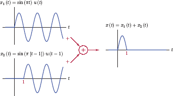
Mathematically we have
Recall that the Laplace transform of a causal sinusoidal signal was found in Example 7.12 as
Using this result with ω0 = π along with the linearity of the Laplace transform and the time-shifting property, we obtain the transform as
which matches the result found earlier.
Software resources:
ex_7_14.m
7.3.3 Shifting in the s-domain
Proof: Through direct application of the Laplace transform definition given by Eqn. (7.1) we get
Let the ROC for original transform X (s) be
For X (s − s0) to converge, we need
Therefore, the ROC for X (s − s0) is
The ROC for X (s − s0) is a shifted version of the ROC for X (s), shifted horizontally by an amount equal to the real part of the parameter s0. This is illustrated in Fig. 7.26.

The effect of s-domain shifting on the ROC: (a) the ROC for X (s), (b) the ROC for X (s − s0).
Example 7.15: Laplace transform of exponentially damped sinusoidal signal
Determine the Laplace transform of the signal
Solution: The transform can be found easily by the use of the s-domain shifting property. Let the signal x1 (t) be defined as
so that
The Laplace transform of a causal cosine signal was derived in Example 7.11. Using the result found in that example with ω0 = 3 yields
We are now ready to apply the s-domain shifting property.
The resulting transform has a zero at s = −2 and a pair of complex conjugate poles at s = −2 ± j3 as shown in Fig. 7.27. The boundary for the ROC is set by the two poles, therefore the ROC is

7.3.4 Scaling in time and s-domains
Given the transform pair
and a real-valued parameter a, the following is also a valid transform pair:
Proof: Once again, we will begin by applying the Laplace transform definition given by Eqn. (7.1) to obtain
If a > 0, employing a variable change λ = at and its consequence dλ = a dt on the integral of Eqn. (7.63) leads to
On the other hand, if a < 0, the same variable change leads to
The reason for the negative sign in Eqn. (7.65) is that, for a < 0, the integration limits for t → ±∞ translate to limits λ → ±∞. In order to account for both possibilities of a > 0 and a < 0, the results in Eqns. (7.64) and (7.65) may be combined to yield
The use of the absolute value on the scale factor eliminates the need for the negative sign when a < 0. This completes the proof of the scaling property given by Eqn. (7.62).
The ROC of the result still needs to be related to the ROC for the original transform X (s). Let the latter be
For the term X (s/a) in Eqn. (7.66) to converge, we need
Since the parameter a is real-valued, the ROC in Eqn. (7.67) can be written as
Depending on the sign of the parameter a, two possibilities need to be considered for the ROC of ℒ{x (at)}:
Example 7.16: Using the scaling property of the Laplace transform
Use the scaling property to find the Laplace transform of the signal
from the knowledge of the transform pair
Solution: It is obvious from a comparison of the signals x (t) and g (t) that
so that the scaling property given by Eqn. (7.62) can be used with the scale factor a = −1 to yield
and the ROC is
The result found is consistent with Eqn. (7.23).
7.3.5 Differentiation in the time domain
Given the transform pair
the following is also a valid transform pair:
Proof: Using the Laplace transform definition in Eqn. (7.1), the transform of dx (t) /dt is
Integrating Eqn. (7.70) by parts yields
The term x (t) e−st must evaluate to zero for t → ± ∞ for the transform X (s) to exist. Therefore, Eqn. (7.71) reduces to
completing the proof.
The ROC for the transform of dx (t) /dt is at least equal to the ROC of the original transform. If the original transform X (s) has a single pole at s = 0 that sets the boundary of its ROC, then the cancellation of that pole due to multiplication by s causes the ROC of the new transform sX (s) to be larger.
Example 7.17: Using the time-domain differentiation property of the Laplace transform
Use the time-domain differentiation property to find the Laplace transform of the signal
from the knowledge of the transform pair
Solution: Let us differentiate the signal g (t):
Based on the result in Eqn. (7.73), the signal x (t) can be written as
and its Laplace transform is
as expected. The ROC of X (s) is
7.3.6 Differentiation in the s-domain
Given the transform pair
the following is also a valid transform pair:
Proof: The proof is straightforward by differentiating both sides of the Laplace transform definition given by Eqn. (7.1):
Interchanging the order of integration and differentiation on the right side of Eqn. (7.75) leads to
Eqn. (7.74) follows from Eqn. ((7.76).
The ROC for the transform of tx (t) is the same as the ROC for the original transform X (s).
Example 7.18: Using the s-domain differentiation property of the Laplace transform
Determine the Laplace transform of the unit-ramp signal
Solution: The Laplace transform of the unit-step function is
Using the s-domain differentiation property, the Laplace transform of the unit-ramp signal is
and the ROC of the transform is
Example 7.19: Transform of a signal using multiple ramp functions
Determine the Laplace transform of the signal x (t) shown in Fig. 7.28.
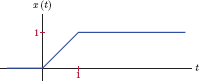
Solution: The signal x (t) can be expressed in terms of a unit-ramp function and its delayed version as
The transform of the unit-ramp function was determined in Example 7.18. Using the result in Eqn. (7.77) along with the time-shifting property we obtain
with the ROC
Example 7.20: Transform of an exponentially damped ramp function
Determine the Laplace transform of the signal
which is shown in Fig. 7.29.
Solution: The transform of the causal exponential signal e−2t u (t) is
Using the s-domain differentiation property
with the ROC
7.3.7 Convolution property
For any two signals x1 (t) and x2 (t) with their respective transforms
and
it can be shown that the following transform relationship holds:
Convolution property of the Laplace transform is fundamental in its application to CTLTI systems.
Proof: The proof will be carried out by using the convolution result inside the Laplace transform definition. The convolution of two continuous-time signals x1 (t) and x2 (t) is given by
Substituting Eqn. (7.79) into the Laplace transform definition leads to
Interchanging the order of the two integrals, Eqn. (7.80) can be written as
We will focus our attention on the inner integral in Eqn. (7.81). Using the time-shifting property it follows that
Substituting Eqn. (7.82) into Eqn. (7.81) we obtain
As before, the ROC for the resulting transform is at least the overlap of the ROCs of two individual transforms, if such an overlap exists. It may be greater than the overlap of the two ROCs if the multiplication of X1 (s) and X2 (s) results in the cancellation of a pole that determines the boundary of one of the ROCs.
Convolution property of the Laplace transform is very useful in the sense that it provides an alternative to computing the convolution of two signals directly in the time-domain. Instead, the convolution result x (t) = x1 (t) * x2 (t) can be obtained using the procedure outlined below:
Finding convolution result through the Laplace transform:
To compute x (t) = x1 (t) * x2 (t):
Find the Laplace transforms of the two signals.
Multiply the two transforms to obtain X (s).
Compute x (t) as the inverse Laplace transform of X (s).
Example 7.21: Using the convolution property of the Laplace transform
Consider two signals x1 (t) and x2 (t) given by
and
Determine
using Laplace transform techniques.
Solution: Individual transforms of the signals x1 (t) and x2 (t) are
and
Applying the convolution property, the transform of x (t) is the product of the two transforms:
The overlap of the two ROCs in Eqns. (7.84) and (7.85) would be Re {s} > −1; however, the pole at s = −1 is cancelled in the process of multiplying the two transforms. Consequently, the ROC for X (s) is
as shown in Fig. 7.30.

The signal x (t) is the inverse Laplace transform of X (s):
7.3.8 Integration property
Given the transform pair
the following is also a valid transform pair:
Proof: Let a new signal be defined from x (t) as
Using the definition of the Laplace transform in conjunction with the signal w (t) we get
which would be difficult to evaluate directly. Instead, we will make use of other properties of the Laplace transform discussed earlier. Differentiating both sides of Eqn. (7.87) we get
Using the time-domain differentiation property of the Laplace transform, Eqn. (7.88) leads to the relationship
from which the desired result is obtained:
An alternative method of proving the integration property will be presented to provide further insight. Let us write the convolution of x (t) with the unit-step function:
We know that
Therefore, we can set the upper limit of the integral in Eqn. (7.90) to λ = t and drop the unit-step function without changing the integration result. Doing so leads to
Since w (t) is equal to the convolution of x (t) and the unit-step function, its Laplace transform must be equal to the product of the respective transforms:
The ROC may need to be adjusted. Let the ROC of the original transform X (s) be
The ROC for the Laplace transform of the unit-step function is
Therefore, the ROC of the transform W (s) must be at least the overlap of these regions. It may be larger than the overlap if X (s) has a zero at s = 0 to counter the pole at s = 0 introduced by the transform of the unit-step function.
7.4 Inverse Laplace Transform
Consider a transform pair
If X (s) is given, the signal x (t) can be found using the inverse Laplace transform
The contour C is a vertical line within the ROC of the transform as shown in Fig. 7.31.

Even though the contour integral in Eqn. (7.93) will not be used in this text for the actual computation of the inverse Laplace transform, it will be explored a bit further to provide insight.
Consider the Laplace transform X (s) evaluated at s = σ + jω, first given by Eqn. (7.5) and repeated below.
The integral on the right side represents the Fourier transform of the modified signal x (t) e−σt provided that it exists. Let us assume that the point s = σ + jω is in the ROC of X (s) to satisfy the existence condition. The signal x (t) e−σt can be found using the inverse Fourier transform:
Multiplying both sides of Eqn. (7.94) by eσt yields
Substituting
into Eqn. (7.95) we obtain
which is the contour integral given by Eqn. (7.93). The integral needs to be carried out at points on a vertical line in the ROC of the transform.
For a rational function X (s) it is usually easier to compute the inverse Laplace transform through the use of partial fraction expansion (PFE).
7.4.1 Partial fraction expansion with simple poles
Consider a rational transform in the form
where the poles p1,p2,... ,p N are distinct. Furthermore, let the order of the numerator polynomial B (s) be less than N, the order of the denominator polynomial. The transform X (s) can be expanded into partial fractions in the form
The coefficients k1,k2,...,k N are called the residues of the partial fraction expansion. They can be computed by (see Appendix E)
Once the residues are determined, the inverse transform of each term in the partial fraction expansion is determined using either Eqn. (7.22) or Eqn. (7.23), depending on the placement of each pole relative to the ROC.
This will be illustrated in the next several examples.
Software resources: See MATLAB Exercise 7.4.
Example 7.22: Inverse Laplace transform using PFE
A causal signal x (t) has the Laplace transform
Determine x (t) using partial fraction expansion.
Solution: Since x (t) is specified to be causal, the ROC of the transform must be to the right of a vertical line. X (s) has poles at s = −2 and s = 0, therefore the ROC is
Partial fraction expansion of X (s) is in the form
Residues are found by the application of residue formulas:
Using the values found, X (s) is
Both terms of X (s) in Eqn. (7.101) correspond to causal terms in the time domain. Use of the transform pair given by Eqn. (7.22) for both terms yields
Software resources:
ex_7_22a.m
ex_7_22b.m
Example 7.23: Using PFE with complex poles
The Laplace transform of a signal x (t) is
with the ROC specified as
Determine x (t).
Solution: The transform X (s) can be written in factored form as
and expanded into partial fractions as
The residues are determined using the residue formulas. The residues associated with complex poles at ±j3 will be complex-valued, however, the method used for computing them is the same.
The residue k3 can be computed using the same method, however, there is a shortcut available. Since the transform X (s) is a rational function with real coefficients, residues of complex conjugate poles must be complex conjugates of each other. Therefore
Based on the specified ROC, the signal x (t) is causal. Using Eqn. (7.22) for inverting each term of the partial fraction expansion we get
which can be simplified as
An alternative approach would be to combine the two partial fractions with complex poles into a second-order term and write Eqn. (7.102) as
Afterwards the transform pairs
can be used for arriving at the same result.
Software resources:
ex_7_23a.m
ex_7_23b.m
Example 7.24: Using PFE in conjunction with the ROC
The Laplace transform of a signal x (t) is
with the ROC specified as
Determine x (t).
Solution: We will first find the partial fraction expansion of X (s). The ROC will be taken into consideration in the next step. Partial fraction expansion of X (s) is in the form
The residues are
The completed form of the partial fraction expansion is
Next we need to pay attention to the ROC which is a vertical strip in the s-plane between the poles at s = −1 and s = 2 as shown in Fig. 7.32.
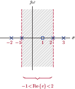
The shape of the ROC indicates a two-sided signal. Accordingly, we will write the transform as the sum of two transforms belonging to causal and anti-causal components of x (t):
The poles at s = −1 and s = −2 are associated with xR (t), the causal component of x (t). Therefore XR (s) can be written as
Conversely the poles at s = 2 and s = 3 are associated with xL (t), the anti-causal component of x (t).
The individual ROCs of the transforms XR (s) and XL (s) are shown in Fig. 7.33(a) and (b).

The signal xR (t) is found by using Eqn. (7.22) on the terms of XR (s):
The signal xL (t) is found by using Eqn. (7.23) on the terms of XL (s):
The signal x (t) is the sum of these two components:
Software resources:
ex_7_24a.m
ex_7_24b.m
If the order of the numerator polynomial B (s) in Eqn. (7.97) is equal to or greater than the order of the denominator polynomial, special precautions need to be taken before partial fraction expansion can be used. In this case X (s) must be written as
where C (s) is a polynomial of S, and the order of the new numerator polynomial is N − 1.
Example 7.25: Using PFE when numerator order is not less than denominator order
The Laplace transform of a causal signal is
Determine x (t).
Solution: Since the numerator order is equal to the denominator order, X (s) cannot be expanded into partial fractions directly. Let us first multiply numerator and denominator
Let X1 (s) be defined as
so that X (s) = 1 + X1 (s). Expanding X1 (s) into partial fractions yields
Consequently we have
and
Software resources:
ex_7_25a.m
ex_7_25b.m
7.4.2 Partial fraction expansion with multiple poles
If the transform X (s) has repeated roots, residue calculations become a bit more complicated. Consider a rational transform in the form
The pole of multiplicity r at s = p1 requires r terms in the partial fraction expansion:
The residues of single poles at p2,...,pN are still computed using the residue formulas discussed earlier in the previous section. The residue k1,r is also easy to compute:
The residue k1,r−1 for the partial fraction with (s − p1)r − 1 in its denominator requires more work, and is computed as
The residue k1, r−2 is
and so on. See Appendix E for details.
Example 7.26: Multiple-order poles
A causal signal x (t) has the Laplace transform
Determine x (t) using partial fraction expansion.
Solution: The partial fraction expansion for X (s) is in the form
The residue k2 for the single pole at s = 2 is easily determined using the residue formula:
The residues of the third-order pole at s = −1 are found using Eqns. (7.107) through
and the partial fraction expansion of X (s) is
Using the transform pairs
and
to invert the terms of the partial fraction expansion, we arrive at the solution
Software resources:
ex_7_26.m
See MATLAB Exercises 7.4 and 7.5. |
7.5 Using the Laplace Transform with CTLTI Systems
We have shown in Chapter 2 that the output signal of a CTLTI system can be computed from its input signal and its impulse response through the use of the convolution integral. If the impulse response of a CTLTI system is h (t), and if the signal x (t) is applied to the system as input, the output signal y (t) is found as
Based on the convolution property of the Laplace transform introduced in Eqn. (7.78) in Section 7.3.7, the transform of the convolution of two signals is equal to the product of their individual transforms. Therefore, the transform of the output signal is
As an alternative to computing the output signal by direct application of the convolution integral, we could
- Find the Laplace transforms of the input signal x (t) and the impulse response h (t).
- Multiply the two transforms to obtain the transform Y (s).
- Determine the output signal y (t) from Y (s) by means of the inverse Laplace transform.
Solving Eqn. (7.110) for H (s) we get
The function H (s) is the s-domain system function of the system under consideration.
If the input and the output signals x (t) and y (t) are specified, the impulse response of the CTLTI system can be found by
Finding the Laplace transform of each.
Finding the transform H (s) as the ratio of the two, as given by Eqn. (7.111).
Using the inverse Laplace transform operation on H (s).
We already know that a CTLTI system can be completely and uniquely described by means of its impulse response h (t). Since the system function H (s) is just the Laplace transform of the impulse response h (t), it also represents a complete description of the CTLTI system.
7.5.1 Relating the system function to the differential equation
As discussed in Section 2.4 of Chapter 2, the input-output relationship of a CTLTI system can be modeled by a constant-coefficient linear differential equation given in the standard form
The order of the CTLTI system is the larger of M and N. Up to this point we have considered three different forms of modeling for a CTLTI system, namely the differential equation, the impulse response and the system function. (A fourth method, state-space modeling, will be introduced in Chapter 9.) It must be possible to obtain any of the three models from the knowledge of any other. In this section we will focus on the problem of determining the system function from the differential equation. If we take the Laplace transform of both sides of Eqn. (7.112) the equality would still be valid:
Laplace transform is linear; therefore, the transform of a summation is equal to the sum of individual terms, allowing us to write Eqn. (7.113) as
and subsequently as
Using the time-domain differentiation property of the Laplace transform, given by Eqn. (7.69), in Eqn. (7.115) yields
The transforms X (s) and Y (s) do not depend on the summation indices k, and can therefore be factored out of the summations in Eqn. (7.116) resulting in
The system function can now be obtained from Eqn. (7.117) as
Finding the system function from the differential equation:
Separate the terms of the differential equation so that y (t) and its derivatives are on the left of the equal sign, and x (t) and its derivatives are on the right of the equal sign, as in Eqn. (7.112).
Take the Laplace transform of each side of the differential equation, and use the time-differentiation property of the Laplace transform as in Eqn. (7.116).
Determine the system function as the ratio of Y (s) to X (s) as in Eqn. (7.118).
If the impulse response is needed, it can now be determined as the inverse Laplace transform of H (s).
System function, linearity, and initial conditions
Two important observations will be made at this point:
The development leading up to the s-domain system function in Eqn. (7.111) has relied heavily on the convolution operation and the convolution property of the Laplace transform. We know from Chapter 2 that the convolution operation is only applicable to problems involving linear and time-invariant systems. Therefore it follows that the system function concept is meaningful only for systems that are both linear and time-invariant. This notion was introduced in earlier discussions involving system functions as well.
Furthermore, it was justified in Section 2.4 of Chapter 2 that a constant-coefficient differential equation corresponds to a linear and time-invariant system only if all initial conditions are set equal to zero.
We conclude that, in determining the system function from the differential equation, all initial conditions must be assumed to be zero.
If we need to use Laplace transform-based techniques to solve a differential equation subject to non-zero initial conditions, that can be done through the use of the unilateral Laplace transform, but not through the use of the system function. The unilateral Laplace transform and its use for solving differential equations will be discussed in Section 7.7.
Example 7.27: Finding the system function from the differential equation
A CTLTI system is defined by means of the differential equation
Find the system function H (s) for this system.
Solution: We will assume that all initial conditions are equal to zero, and take the Laplace transform of each side of the differential equation to obtain
The system function can be obtained from Eqn. (7.119) as
Characteristic polynomial vs. the denominator of the system function
Another important observation will be made based on the result obtained in Example 7.27: The characteristic equation for the system considered in Example 7.27 is
and the solutions of the characteristic equation are the modes of the system as defined in Section 2.5.3 of Chapter 2. When we find the system function H (s) from the differential equation we see that its denominator polynomial is identical to the characteristic polynomial. The roots of the denominator polynomial are the poles of the system function in the s-domain, and consequently, they are identical to the modes of the differential equation of the system.
Recall that in Section 2.5.3 we have reached some conclusions about the relationship between the modes of the differential equation and the natural response of the corresponding system. The same conclusions would apply to the poles of the system function. Specifically, if all poles of the system are real-valued and distinct, then the transient response of the system is in the form
Complex poles appear in conjugate pairs provided that all denominator coefficients of the system function are real-valued. A pair of complex conjugate poles
yields a response of the type
Finally, a pole of multiplicity m at s = p1 leads to a response in the form
regardless of whether p1 is real or complex-valued. Justifications for these relationships were given in Section 2.5.3 of Chapter 2 through the use of the modes of the differential equation, and will not be repeated here.
Sometimes we need to reverse the problem represented in Example 7.27 and find the differential equation from the knowledge of the system function. The next three examples will demonstrate this.
Software resources: See MATLAB Exercises 7.5.
Example 7.28: Finding the differential equation from the system function
A causal CTLTI system is defined by the system function
Find a differential equation for this system.
Solution: The system function is the ratio of the output transform to the input transform, that is,
Therefore we can write
The differential equation follows from Eqn. (7.120) as
Example 7.29: Finding the differential equation from input and output signals
The unit-step response of a CTLTI system is
Find a differential equation for this system.
Solution: Since the input signal is a unit-step function, that is, x (t) = u (t), its Laplace transform is
The Laplace transform of the output signal is found as
The system function can be obtained as the ratio of the output transform to the input transform:
The differential equation follows from the system function as
Software resources:
ex_7_29.m
Example 7.30: Finding the impulse response from input and output signals
Determine the impulse response of the CTLTI system system the unit-step response of which was given in Example 7.29.
Solution: The system function was found in Example 7.29 to be
which can be expanded into partial fractions to yield
It can be easily verified that the unit-step response specified in Example 7.29 for this system is indeed the convolution of h (t) found above with the unit-step function.
Software resources:
ex_7_30.m
7.5.2 Response of a CTLTI system to a complex exponential signal
In this section we will consider the response of a CTLTI system to a complex exponential input signal. This will help us gain further insight into the system function concept.
Let a CTLTI system with impulse response h (t) be driven by a complex exponential input signal in the form
where s0 represents a point in the s-plane within the ROC of the system function. The output signal can be determined through the use of the convolution integral
Substituting into Eqn. (7.121) and simplifying the resulting integral we obtain
The integral in Eqn. (7.122) should be recognized as the system function H (s) evaluated at the point s = s0 in the s-plane. Therefore, we reach the following important conclusion:
The response of the CTLTI system to the input signal is
The CTLTI system responds to the complex exponential signal by scaling it with the (generally complex) value of the system function at the point s = s0.
In Eqn. (7.123) the complex exponential input signal is assumed to have been in existence forever; it is not turned on at a specific time instant. Therefore, the response found is the steady-state response of the system.
Example 7.31: Response to a complex exponential signal
A CTLTI system with the system function
is driven by the complex exponential input signal
Determine the steady-state response of the system.
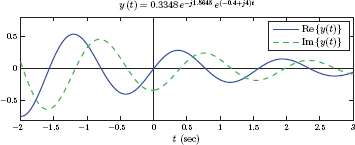
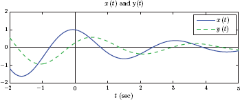
Solution: The input signal is complex-valued, and can be written in Cartesian form using Euler’s formula:
Real and imaginary parts of x (t) are shown in Fig. 7.34.

The value of the system function at s = s0 = −0.4 + j4 is
The output signal is found using Eqn. (7.123) as
or, in Cartesian form as
Real and imaginary parts of the output signal y (t) are shown in Fig. 7.35.
Software resources:
ex_7_31.m
7.5.3 Response of a CTLTI system to an exponentially damped sinusoid
Next we will consider an input signal in the form of an exponentially damped sinusoid
In order to find the response of a CTLTI system to this signal, let us write x (t) using Euler’s formula:
Let the parameter s0 be defined as
so that Eqn. (7.127) becomes
Using the linearity of the system, its response to x (t) can be written as
We already know that the response of the system to the term is
The response to the term is found similarly:
Using Eqns. (7.130) and (7.131) in Eqn. (7.129) the output signal is
It is possible to further simplify the result obtained in Eqn. (7.132). Let the value of the system function evaluated at the point s = s0 be written in polar complex form as
where H0 and θ0 represent the magnitude and the phase of the system function at the point s = s0 respectively:
and
For a real-valued impulse response it can be shown (see Problem 7.27 at the end of this chapter) that the value of the system function at the point is the complex conjugate of its value at the point s = s0, that is,
Using Eqns. (7.133) and (7.136) in Eqn. (7.132), the output signal y (t) becomes
The derivation outlined in Eqns. (7.127) through (7.137) can be summarized as shown in Fig. 7.36.
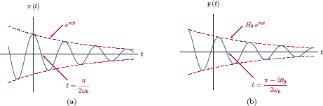
The response of a CTLTI system to an exponentially damped sinusoid: (a) input signal, (b) output signal.
Comparison of the input signal in Eqn. (7.126) and the output signal Eqn. (7.137) reveals the following:
The amplitude of the signal is multiplied by the magnitude of the system function evaluated at the point s = s0 = σ0 + jω0.
The phase of the cosine function is incremented by an amount equal to the phase of the system function evaluated at the point s = s0 = σ0 + jω0.
Example 7.32: Response to an exponentially damped sinusoid
Consider again the system function used in Example 7.31. Determine the response of the system to the input signal
Solution: Let s0 be defined as
The system function evaluated at s = s0 is
or in polar form
The output signal is found using Eqn. (7.137):
The input and the output signals are shown in Fig. 7.37.
Software resources:
ex_7_32.m
7.5.4 Pole-zero plot for a system function
A rational system function H (s) can be expressed in pole-zero form as
The parameters M and N are the numerator order and the denominator order respectively. The larger of M and N is the order of the system. The roots z1,..., zM of the numerator polynomial are referred to as the zeros of the system function. In contrast, the roots of the denominator polynomial are the poles of the system function. A pole-zero plot for a system function is obtained by marking the poles and the zeros of the system function on the s-plane. It is customary to use “x” and “o” to mark each pole and each zero respectively.
Example 7.33: Pole-zero plot for system function
Construct a pole-zero plot for a CTLTI system with system function
Solution: The zeros of the system function are the roots of the numerator polynomial, and are found by solving the equation
which yields z1 = j and z2 = −j. The poles of the system function are the roots of the denominator polynomial or, equivalently, the solutions of the equation
The three poles are at p1 = −1, p2 = −2 + j3 and p3 = −2 − j3. The pole-zero diagram for the system function is shown in Fig. 7.38.

Software resources:
ex_7_33.m
Example 7.34: ROC and the pole-zero plot
Assume that the system function used in Example 7.33 represents a causal system. Indicate the ROC on the pole-zero plot.
Solution: Following is the knowledge we possess:
For a causal system, the ROC of the system function must be the area to the right of a vertical line.
The ROC must be bound by one or more poles.
There may be no poles within the ROC.
Consequently, the ROC of the system function must be
which is shown in Fig. 7.39.
7.5.5 Graphical interpretation of the pole-zero plot
In this section we will explore the significance of the geometric placement of poles and zeros of the system function. The pole-zero plot, introduced in Section 7.5.4, can be used for understanding the behavior characteristics of a CTLTI system, especially in terms of the magnitude and the phase of the system function. The relationship between the locations of the poles and the zeros of the system function and the frequency-domain behavior of the system is significant.
Let us begin by considering the pole-zero form of the system function given by Eqn. (7.138). Assuming the system is stable, the Fourier transform-based system function H (ω) exists, and can be found by evaluating H (s) for s = jω:
The numerator of Eqn. (7.139) has M factors each in the form
Similarly, the denominator of Eqn. (7.139) consists of factors in the form
In a sense, the function Bi (ω) describes the contribution of the zero at s = zi to the frequency response of the system. Similarly, the function Ai (ω) describes the contribution of the pole at s = pi. Using the definitions in Eqns. (7.140) and (7.141), H (ω) becomes
If we wanted to compute the frequency response of the system at a specific frequency ω = ω0 we would get
The magnitude of the frequency response at ω = ω0 is found by computing the magnitude of each complex function Bi (ω0) and Ai (ω0), and forming the ratio
The phase of the frequency response is computed as the algebraic sum of the phases of numerator and denominator factors:
We would like to gain a graphical understanding of the computations in Eqns. (7.144) and (7.145). Let us focus on one of the numerator terms, Bi (ω0):
Clearly, B (ω0) is a complex quantity. Its two terms zi and jω0 are shown in Fig. 7.40(a) as points in the s-plane. It is also possible to represent the terms in Eqn. (7.146) with vectors. Treating each term in Eqn. (7.146) as a vector, we obtain the corresponding vector expression
which can be written in alternative form

(a) The zero s = zi and the point s = jω0 in the complex plane, (b) the vectors for zi and jω0 in the complex plane, (c) the relationship expressed by Eqn. (7.148).
We will draw the vector starting at the origin and ending at the point s = zi. Similarly the vector will be drawn starting at the origin and ending at the point s = jω0. These two vectors are shown in Fig. 7.40(b). The relationship expressed by Eqn. (7.148) is illustrated in Fig. 7.40(c). The following important conclusions can be drawn from Fig. 7.40(c):
- The vector is drawn starting at the zero at s = zi and ending at the point s = jω0 on the jω-axis.
- The magnitude is equal to the norm of the vector .
- The phase is equal to the angle that the vector makes with the positive real axis, measured counterclockwise.
If Fig. 7.40(c) is drawn to scale, the norm and the angle of the vector could simply be measured to determine the contributions of the zero at s = zi to the magnitude and the phase expressions for and in Eqns. (7.144) and (7.145).
What if we need to determine the contributions of the zero at s = zi to the magnitude and phase not just for a specific frequency ω0 but for all frequencies ω? Imagine the vector to be a piece of rubber band, the tail end of which is permanently attached to the point s = zi. Assume that, as the frequency ω varies, the tip of the rubber band vector moves on the jω-axis. The length of the rubber band and its angle with the positive real axis vary as the tip is moved. The contributions of the zero at s = zi to the magnitude and the phase of the frequency response H (ω) can be graphed by tracking these variations as shown in Fig. 7.41.
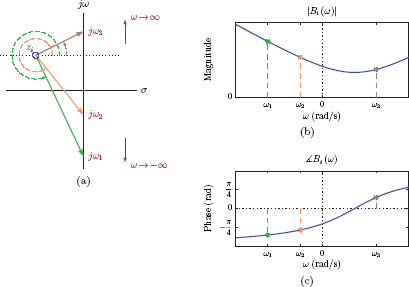
(a) Moving the tip of the vector for Bi (ω) on the jω-axis using the rubber band analogy, (b) contribution of the zero at s = zi to the magnitude of the frequency response, (c) contribution of the zero at s = zi to the phase of the frequency response.
Similar analysis can be carried out for determining the contribution of a pole pi to magnitude and phase characteristics of the system. Fig. 7.42 illustrates the effect of a pole on the frequency response.

(a) Moving the tip of the vector for Ai (ω) on the jω-axis using the rubber band analogy, (b) contribution of the pole at s = pi to the magnitude of the frequency response, (c) contribution of the pole at s = pi to the phase of the frequency response.
For a system with M zeros and N poles, magnitude and phase of the system function at ω = ω0 are found by taking into account the contributions of each zero and pole. The next example will illustrate this.
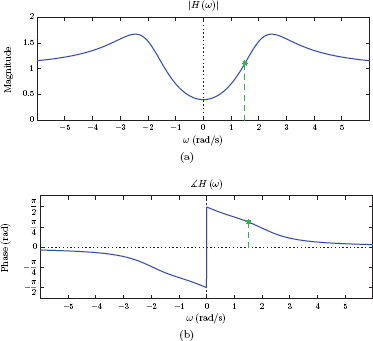
Example 7.35: Frequency response from pole-zero plot
A CTLTI system is described by the system function
Construct a pole-zero plot and use it to determine the magnitude and the phase of the frequency response of the system at the frequency ω0 = 1.5 rad/s.
Solution: The system has two zeros and two poles. The zeros of the system function are at
and the poles are at
Vector forms of the contribution of each zero and pole to the system function at ω = ω0
can be written using Eqns. (7.140) and (7.141) as
The vectors , , , and are shown in Fig.7.43.

The norm and the phase of each vector are
Based on the values measured, the magnitude of the frequency response at ω0 is computed as
The phase of the frequency response is computed as
Complete magnitude and phase characteristics for the system can be obtained by repeating this process for all values of ω that are of interest. Fig. 7.44 shows the magnitude and the phase of the system. The values at ω0 = 1.5 rad/s are marked on magnitude and phase plots.
Software resources:
ex_7_35.m
Software resources: |
See MATLAB Exercises 7.6 and 7.7. |
Interactive Demo: pz_demo1.m
The pole-zero explorer demo program “pz_demol.m” allows experimentation with the placement of poles and zeros of the system function. Before using it two vectors should be created in MATLAB workspace: one containing the poles of the system and one containing its zeros. In the pole-zero explorer user interface, the “import” button is used for importing these vectors. Pole-zero layout in the s-plane is displayed along with the magnitude and the phase of the system function. The vectors from each zero and each pole to a point on the jω-axis may optionally be displayed. Individual poles and zeros may be moved, and the effects on magnitude and phase may be observed. Complex conjugate poles and zeros move together to keep the conjugate relationship.
As an example, the system in Example 7.32 may be duplicated by creating and importing the two vectors
Software resources:
pz_demo1.m
7.5.6 System function and causality
Causality in linear and time-invariant systems was discussed in Section 2.8 of Chapter 2. For a CTLTI system to be causal, its impulse response h (t) needs to be equal to zero for t < 0. Thus, by changing the lower limit of the integral to t = 0 in the definition of the Laplace transform, the s-domain system function for a causal CTLTI system can be written as
As we have discussed in Section 7.2 of this chapter, the ROC for the system function of a causal system is to the right of a vertical line in the s-plane. As a consequence, the system function must also converge at Re {s} → ∞. Consider a system function in the form
For the system described by H (s) to be causal we need
which requires that M − N ≤ 0 and consequently M ≤ N. Thus we arrive at an important conclusion:
Causality condition:
In the s-domain system function of a causal CTLTI system the order of the numerator must not be greater than the order of the denominator.
Note that this condition is necessary for a system to be causal, but it is not sufficient. It is also possible for a non-causal system to have a system function with M ≤ N.
7.5.7 System function and stability
In Section 2.9 of Chapter 2 we have concluded that for a CTLTI system to be stable its impulse response must be absolute integrable, that is,
Furthermore, we have established in Section 4.3.2 of Chapter 4 that the Fourier transform of a signal exists if the signal is absolute integrable. But the Fourier transform of the impulse response is equal to the s-domain system function evaluated on the jω-axis of the s-plane, that is,
provided that the jω-axis of the s-plane is within the ROC.
Stability condition:
Therefore, it follows that, for a CTLTI system to be stable, the ROC of its s-domain system function must include the jω-axis.
What are the corresponding conditions that must be imposed on the locations of poles and zeros for stability? We will answer this question by taking three-separate cases into account:
Causal system:
The ROC for the system function of a causal system is to the right of a vertical line in the s-plane, and is expressed in the form
For the ROC to include the jω-axis we need σ1 < 0. Since the ROC cannot have any poles in it, all the poles of the system function must be on or to the left of the vertical line σ = σ1.
For a causal system to be stable, the system function must not have any poles on the jω-axis or in the right half s-plane.
Anti-causal system:
If the system is anti-causal, its impulse response is equal to zero for t ≥ 0. The ROC for the system function is to the left of a vertical line in the s-plane, and is expressed in the form
For the ROC to include the jω-axis we need σ2 > 0. All the poles of the system function must reside on or to the right of the vertical line σ = σ2.
For an anti-causal system to be stable, the system function must not have any poles on the jω-axis or in the left half s-plane.
Neither causal nor anti-causal system:
In this case the ROC for the system function, if it exists, is the region between two vertical lines at σ = σ1 and σ = σ2, and is expressed in the form
For stability we need σ1 < 0 and σ2 > 0. The poles of the system function may be either
- On or to the left of the vertical line σ = σ1
- On or to the right of the vertical line σ = σ2
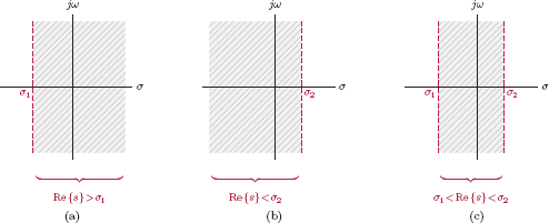
The ROC for a stable system that is (a) causal, (b) anti-causal, (c) neither causal nor anti-causal.
Example 7.36: Impulse response of a stable system
A stable system is characterized by the system function
Determine the ROC of the system function. Afterwards find the impulse response of the system.
Solution: The ROC for the system function is not directly stated; however, we are given enough information to deduce it. The three poles of the system function are at s = −3, 1, 2. Since the system is known to be stable, its ROC must include the jω-axis of the s-plane. The only possible choice is
as shown in Fig. 7.46(a). Partial fraction expansion of H (s) is

Based on the ROC determined above, the first term in the partial fraction expansion corresponds to a causal signal, and the other two terms correspond to anti-causal signals. The impulse response of the system is
which is shown in Fig. 7.46(b). We observe that h (t) tends to zero as t is increased in both directions, consistent with the fact that h (t) must be absolute summable for a stable system.
Software resources:
ex_7_36a.m
ex_7_36b.m
Example 7.37: Stability of a system described by a differential equation
A causal CTLTI system is characterized by the differential equation
Determine if the system is stable.
Solution: The ROC for the system function is not directly stated. On the other hand, we are told that the system is causal. This bit of information should allow us to determine the ROC. Taking the Laplace transform of both sides of the differential equation and using the time differentiation property we have
The system function is found by forming the ratio of the output and the input transforms.
The system has a zero at s = −1 and a pair of complex conjugate poles at s = −1 ± j1. Since it is causal, the ROC must be to the right of a vertical line going through σ = −1, that is
Since the ROC includes the jω-axis of the s-plane, the system is stable. The impulse response can be determined easily by writing the H (s) in the form
Using s-domain shifting property of the Laplace transform it follows that

(a) Pole-zero diagram and ROC for the system of Example 7.37, (b) impulse response h (t).
Software resources:
ex_7_37a.m
ex_7_37b.m
7.5.8 Allpass systems
A system the magnitude characteristic of which is constant across all frequencies is called an allpass system. For a system to be considered an allpass system we need
Consider a first-order CTLTI system with a pole at p1 = −σi + j0 and a zero at z1 = σ1 + j0 so that the system function is
For the system to be causal and stable the parameter σ1 needs to be positive so that the resulting pole is in the left half s-plane. The magnitude and the phase of the system function can be expressed using the conventions established in Section 7.5.5. The frequency response H (ω) is found by substituting s = jω:
The magnitude of the frequency response is
The phases of numerator and denominator terms are
and the phase of the frequency response is
The pole-zero diagram and the vector representation of the system function are shown in Fig. 7.48(a) along with the vectors

(a) Pole-zero diagram for first-order allpass system in Eqn. (7.156), (b) phase response of the first-order allpass system.
Fig. 7.48(b) shows the phase characteristics for σ1 = 1, σ1 = 2 and σ1 = 3.
Since the shape of the phase response can be controlled by the choice of parameter σ1 while keeping the magnitude response constant, an allpass system is also referred to as a phase-shifter. Increased versatility in controlling the phase response can be obtained by choosing the pole and the zero to be complex-valued. Consider a first-order system with a pole at p1 = −α1 + jω1 and a zero at z1 = σ1 + jω1. Again we choose σ1 > 0 to obtain a system that is both causal and stable. The corresponding system function is
The frequency response of the system, found by substituting s = jω into the system function, is
It is a trivial matter to show that the magnitude of H (ω) is still equal to unity. Its phase
The pole-zero diagram and the vector representation of the system function are shown in Fig. 7.49(a) along with the vectors

(a) Pole-zero diagram for first-order allpass system in Eqn. (7.162), (b) phase response of the first-order allpass system.
The phase response is shown in Fig. 7.49(b) for ω1 = 1.5 rad/s and for three different values of σ1, namely σ1 = 1, σ1 = 2 and σ1 = 3.
Naturally, the system function in Eqn. (7.162) has complex coefficients. If an allpass system with real coefficients is desired, complex poles and zeros must occur in conjugate pairs. A second-order system with zeros at z1, 2 = σ1 ± jω1 and poles at p1, 2 = −σ1 ± jω1 has allpass characteristics. As before, σ1 > 0 for a causal and stable system. The system function is
The pole-zero diagram for a second-order allpass system is shown in Fig. 7.50(a). The phase response is shown in Fig. 7.50(b) for ω1 = 1.5 rad/s and for three different values of σ1.
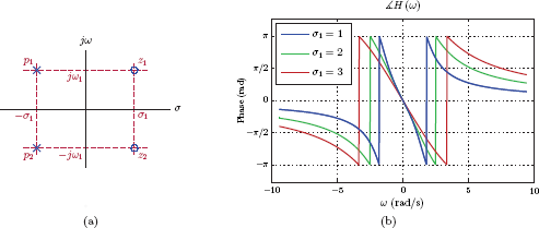
(a) Pole-zero diagram for second-order allpass system in Eqn. (7.166), (b) phase response of the second-order allpass system.
7.5.9 Inverse systems
The inverse of a system is another system which, when connected in cascade with the original system, forms an identity system. This relationship is depicted in Fig. 7.51.

The output signal of the original system is
We require the inverse system to recover the original input signal x (t) from the output signal y (t), therefore
Combining Eqns. (7.166) and (7.166) yields
Let the original system and its inverse be both CTLTI systems with impulse responses h (t) and hi (t) respectively as shown in Fig. 7.52. For the output signal of the inverse system to be identical to the input signal of the original system, the impulse response of the cascade combination must be equal to δ (t), that is,
or, using the convolution integral
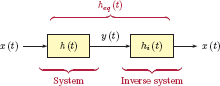
The corresponding relationship between the system functions of the original system and the inverse system is found by taking the Laplace transform of Eqn. (7.169):
Consequently, the system function of the inverse system is
Two important characteristics of the inverse system are causality and stability. We will first focus on causality. Consider the system H (s) function in the form
The system function for the inverse system is
If the original system with system function H (s) is causal then M ≤ N as we have established in Section 7.5.6. By the same token, causality of the inverse system with system function Hi (s) requires N ≤ M. Hence we need N = M if both the original system and its inverse are required to be causal.
To analyze the stability of the inverse system we will find it more convenient to write the system function H (s) in pole-zero form. Using M = N we have
If the original system is both causal and stable, all its poles must be in the left half s-plane (see Section 7.5.7), therefore
The system function of the inverse system, written in pole-zero form, is
For the inverse system to be stable, its poles must also lie in the left half s-plane. The poles of the inverse system are the zeros of the original system. Therefore, for the inverse system to be stable, both zeros and poles of the original system must be in the left half s-plane. In addition to Eqn. (7.175) we also need
A causal CTLTI system that has all of its zeros and poles in the left half s-plane is referred to as a minimum-phase system. A minimum-phase system and its inverse are both causal and stable.
Example 7.38: Inverse of a system described by a differential equation
A causal CTLTI system is described by a differential equation
Determine if a causal and stable inverse can be found for this system. If yes, find a differential equation for the inverse system.
Solution: Taking the Laplace transform of both sides of the differential equation we get
The system function for the original system is
The system function for the inverse system is found as the reciprocal of H (s):
The inverse system is also causal and stable. It leads to the differential equation
7.5.10 Bode plots
Bode plots of the frequency response are used in the analysis and design of feedback control systems. A Bode plot consists of the dB magnitude and the phase , each graphed as a function of . Because of the use of the logarithm, individual contributions of the zeros and the poles of H (s) to the magnitude of the frequency response are additive rather than multiplicative. Also, since is used for the horizontal axis, only positive values of ω are of interest.
Consider again the pole-zero form of the system function H (s) given by Eqn. (7.138). A slightly modified form of it will be more convenient for use in deriving the Bode plot. Let us scale each factor in the numerator and the denominator, and write Eqn. (7.138) as
The new gain factor K1 is chosen to compensate for all the scale factors used in individual terms. The dB magnitude of H (ω) is obtained as
and the phase is
To facilitate the analysis of individual contributions from zeros and poles of the system function, let us write H (s) as a cascade combination of M + N subsystems such that
and
The Bode plot for magnitude and phase can be constructed by computing the contribution of each term in Eqns. (7.182) and (7.183). We will consider four different cases.
Zero at the origin
Let Hk (s) = s. Corresponding dB magnitude and phase are computed as
and
The magnitude characteristic, when graphed as a function of , is a straight line that goes through 0 dB at ω = 1. Its slope is 20 dB per decade.2 This is illustrated in Fig. 7.53(a).
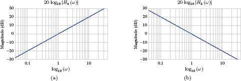
Pole at the origin
Let Hk (s) = 1/s. Corresponding dB magnitude and phase are computed as
and
The magnitude characteristic, when graphed as a function of , is a straight line that goes through 0 dB at ω = 1. Its slope is −20 dB per decade. This is illustrated in Fig. 7.53(b).
Single real zero
Let zk be a real-valued zero of the system. Substituting s = jω into Eqn. (7.182) we obtain
Corresponding dB magnitude is
and the corresponding phase characteristic is
Keep in mind that we need to graph and as functions of , and we are only interested in positive values of ω.
If we have
The magnitude in Eqn. (7.189) can be approximated as
The phase angle can be approximated as
At the opposite extreme, for we have
The magnitude in Eqn. (7.189) can be approximated as
which can also be written in the form
In this case the phase angle depends on the sign of zk:
At the frequency the magnitude is
The phase angle depends on the sign of zk:
The conclusions obtained above can be summarized as follows:
For the term Hk (s) = 1 − s/zk with real-valued zk:
- Magnitude: For the magnitude characteristic is asymptotic to 0 dB. For it becomes asymptotic to a straight line with a slope of 20 dB per decade, which intersects the horizontal axis at . At the frequency the actual magnitude is approximately equal to 3 dB; therefore, the characteristic passes 3 dB above the intersection of the two asymptotes.
- Phase: For the phase is asymptotic to 0 degrees. For the phase is 90 degrees for zk < 0 and −90 degrees for zk > 0. At ω = zk the phase is 45 degrees for zk < 0 and −45 degrees for zk > 0.
This is illustrated in Figs. 7.54 and 7.55.
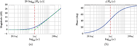
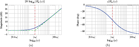
Single real pole
Derivation of the Bode plot for a single real pole is similar. Let pk be a real-valued pole of the system. Substituting s = jω into Eqn. (7.183) yields
and the corresponding phase characteristic is
If we have
The magnitude in Eqn. (7.201) can be approximated as
The phase angle can be approximated as
At the opposite extreme, for we have
The magnitude in Eqn. (7.201) can be approximated as
which can also be written in the form
In this case the phase angle depends on the sign of pk:
At the frequency the magnitude is
The phase angle depends on the sign of pk:
The conclusions obtained above can be summarized as follows:
For the term Hk (s) = 1/(1 − s/pk) with real-valued pk:
Magnitude: For the magnitude characteristic is asymptotic to 0 dB. For it becomes asymptotic to a straight line with a slope of −20 dB per decade, which intersects the 0-dB axis at . At the frequency the actual magnitude is approximately equal to −3 dB, therefore the characteristic passes 3 dB below the intersection of the two asymptotes.
Phase: For the phase is asymptotic to 0 degrees. For the phase is −90 degrees for pk < 0 and 90 degrees for pk > 0. At ω = pk the phase is −45 degrees for pk < 0 and 45 degrees for pk > 0.
This is illustrated in Figs. 7.56 and 7.57.

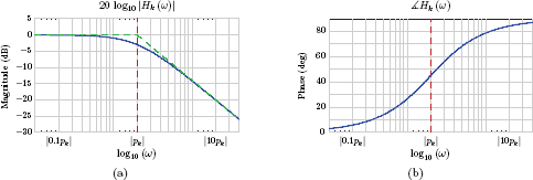
Example 7.39: Constructing a Bode plot
A CTLTI system is described by the system function
Plot the Bode magnitude and the phase characteristics of the system.
Solution: Let us express the system function in the form of four subsystems connected in cascade:
Magnitude and phase contributions of the four subsystems are shown in Fig. 7.58.

Bode plot for the magnitude of the system function is obtained by adding the magnitude contributions in Fig. 7.58(a), (c), (e) and (g). Asymptote lines of the magnitude characteristics can also be added together. Four sections of asymptotes are shown in Fig. 7.59(a) numbered 1 through 4.

Section 1 covers frequencies up to ω = 5 rad/s, and has a slope of 20 dB per decade which is the sum of slopes of all four contributing asymptote lines up to that point. At ω = 5 rad/s, its value is 13.98 dB (see Problem 7.43 at the end of this chapter).
Section 2 covers frequencies from ω = 5 rad/s to ω = 40 rad/s, and has a slope of zero (20 dB per decade from Hi and −20 dB per decade from H3.)
Section 3 covers frequencies from ω = 40 rad/s to ω = 300 rad/s, and has a slope of −20 dB per decade (20 dB per decade from Hi; −20 dB per decade each from H3 and H4). At the endpoint ω = 300 rad/s, its value is −3.52 dB (see Problem 7.43 at the end of this chapter).
Section 4 covers frequencies greater than ω = 300 rad/s, and has a slope of zero (20 dB per decade each from Hi and H2; −20 dB per decade each from H3 and H4).
The actual Bode magnitude plot is also shown in Fig. 7.59. Notice how it passes approximately 3 dB above or below each corner point depending on whether it belongs to a zero or a pole.
Bode plot for the phase of the system function is obtained by adding the phase contributions in Fig. 7.58(b), (d), (f) and (h), and is shown in Fig. 7.59(b).
Software resources:
ex_7_39a.m
ex_7_39b.m
Conjugate pair of poles
Consider a causal and stable second-order system with a pair of complex conjugate poles, that is, . The system function is in the form
H (s) can be written in a slightly different form by multiplying both the numerator and the denominator of Eqn. (7.212) with the product ():
Let us put H (s) into the standard form
with
It follows from Eqn. (7.215) that
Since the system is causal and stable, Re {p1} < 0. Consequently, when the poles of the system form a complex conjugate pair, we have 0 < ζ < 1.
Analysis of the second-order system
The form of the second-order system function given by Eqn. (7.214) can be used for a system with either two real poles or a complex conjugate pair. Let us write H (s) using two poles p1 and p2:
Equating H (s) in Eqn. (7.217) with the form given in Eqn. (7.214) we obtain the relationships
The parameter is called the natural undamped frequency of the system. The parameter ζ is called the damping ratio, and is computed as
The poles of the system function can be related to the parameters ω0 and ζ as
Since the system is causal and stable, both poles are in the left half of the s-plane. As a result the numerator of Eqn. (7.219) is positive, and therefore the damping ratio ζ must be positive. Locations of the poles depend on the value of ζ. We will observe three distinct possibilities:
ζ > 1: The poles p1 and p2 are real-valued and distinct. The system is said to be over-damped.
ζ = 1: The expression in square root in Eqn. (7.220) equals zero. The two poles of the system function are both at p1 = p2 = −ζω0. In this case the system is said to be critically damped.
ζ < 1: The expression in square root in Eqn. (7.220) is negative. The two poles of the system function are a complex conjugate pair:
In this case the system is said to be underdamped.
Fig. 7.60 illustrates the placement of the two poles based on the values of the parameters ζ and ω0.
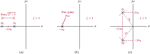
Poles of the second-order system function for (a) ζ > 1, overdamped, (b) ζ = 1, critically damped, (c) ζ < 1, underdamped.
It is also interesting to look at the movement of the two poles as the parameter ζ is changed. Fig. 7.61 illustrates the trajectories of pi and p2.

Let us determine the magnitude and phase responses of the system. Substituting s = jω into Eqn. (7.214) yields
The dB magnitude of the system function is
and the phase characteristic is
If ω ≪ ω0 then we have
If ω ≫ ω0, the dB magnitude becomes
and the phase becomes
It will also be interesting to check the magnitude and the phase at the corner frequency. Substituting ω = ω0 into Eqn. (7.221) we obtain
In this case the phase angle is . Before we compute the dB magnitude at the corner frequency we will define the quality factor as
so that H (ω0) = −jQ. The dB magnitude at ω = ω0 is
The conclusions obtained above can be summarized as follows:
For the second-order system function of Eqn. (7.214):
1.Magnitude: For ω ≪ ω0 the magnitude characteristic is asymptotic to 0 dB. For ω ≫ ω0 it becomes asymptotic to a straight line with a slope of −40 dB per decade, which intersects the 0-dB axis at ω0. At the corner frequency ω = ω0 the actual magnitude is .
2.Phase: For ω ≪ ω0 the phase is asymptotic to 0 degrees. For ω ≫ ω0 it becomes asymptotic to −180 degrees. At the corner frequency ω = ω0 the phase is −90 degrees.
The asymptotic behavior of the dB magnitude characteristic is illustrated in Fig. 7.62 for ω0 = 3 rad/s and for two different values of ζ, namely ζ = 0.1 and ζ = 1.2.
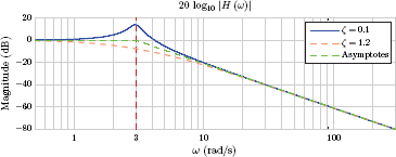
The definitions of overdamped, critically damped and underdamped systems can be related to the new parameter Q as follows:
Bode plots for dB magnitude and phase of the second-order system are shown in Fig. 7.63 for several values of Q.
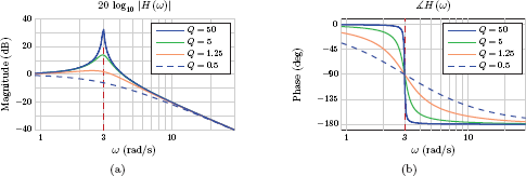
Decibel magnitude and phase characteristics of the second-order system of Eqn. (7.214) for ω0 = 3 rad/s and several values of Q.
The responses of the second-order system to unit-impulse and unit-step input signals are also of interest. Let us use partial fraction expansion to find the impulse response h (t). For the case of two distinct poles (real or complex) the system function H (s) in partial fraction form is
The residues in Eqn. (7.225) are found as
If ζ < 1, the result in Eqn. (7.226) becomes
If ζ = 1 then the expression in Eqn. (7.226) or the one in Eqn. (7.227) will not work since p1 = p2, and the partial fraction expansion in Eqn. (7.225) is not valid in this case. For ζ = 1 we have
Using the s-domain differentiation property of the Laplace transform it can be shown that
The unit-step response can be found by convolving the impulse response found with the unit-step input signal:
For ζ ≠ 1 the use of Eqn. (7.226) in Eqn. (7.229) yields
If ζ = 1, the unit-step response is found by integrating the result Eqn. (7.228):
Impulse response of the system is shown in Fig. 7.64(a) for several values of the damping ratio ζ. Fig. 7.64(b) shows the unit-step response of the system for the same set of values for ζ.

(a) Impulse responses of second-order systems with varying damping ratios, (b) unit-step responses of second-order systems with varying damping ratios.
7.6. Simulation Structures for CTLTI Systems
Development of simulation structures for continuous-time systems was discussed briefly in Section 2.6 of Chapter 2 in the context of obtaining a block diagram from a differential equation. Our discussion in this section will parallel that of Section 2.6, and will utilize the s-domain system function as the starting point.
7.6.1 Direct-form implementation
The method of obtaining a block diagram from an s-domain system function will be derived using a third-order system, but its generalization to higher-order system functions is quite straightforward. Consider a CTLTI system described by a system function H (s).
X (s) and Y (s) are the Laplace transforms of the input and the output signals respectively. Let us use an intermediate function ω (s) and express the system function as
where we have also multiplied both the numerator and the denominator of the system function with s−3 to ensure that no positive powers of s appear. The relationships described by Eqns. (7.232) and (7.233) are illustrated in Fig. 7.65.
![]()
(a) CTLTI system with system function H (s), (b) cascade form using an intermediate function W (s).
If we choose to associate W (s) /X (s) with the denominator of Eqn. (7.233), that is,
then we have
to satisfy Eqn. (7.233). Rearranging the terms in Eqn. (7.234) yields
The relationship in Eqn. (7.236) can easily be translated to a simulation diagram as shown in Fig. 7.66.
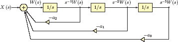
Solving Eqn. (7.235) for the output transform y (s) yields
The terms s−1W (s), s−2W (s) and s−3W (s) are already available in the simulation diagram of Fig. 7.66. Utilizing them to implement the relationship described by Eqn. (7.237), the diagram can be completed as shown in Fig. 7.67.

Using the integration property of the Laplace transform stated by Eqn. (7.86), multiplication by s−1 in the transform domain corresponds to integration of the signal in the time domain. Consequently, the blocks with system function 1/s in the diagram of Fig. 7.67 represent integrators.
It should be noted that the diagram in Fig. 7.67 could easily have been obtained directly from the system function in Eqn. (7.233) by inspection, using the following set of rules:
- Begin by ordering terms of numerator and denominator polynomials from highest to lowest order of s.
- Ensure that the leading coefficient in the denominator, that is, the coefficient of the highest order term, is equal to unity. (If it is not equal to unity, simply scale all coefficients to satisfy this rule.)
- Set gain factors of feed-forward branches equal to the numerator coefficients.
- Set gain factors of feedback branches equal to the negatives of the denominator coefficients.
- Be careful to account for any missing powers of s in either polynomial, and treat them as terms with their coefficients equal to zero.
Example 7.40: Obtaining a block diagram from system function
A CTLTI system is described through the system function
Draw a block diagram for simulating this system.
Solution: Using the technique outlined above, the block diagram shown in Fig. 7.69 is obtained.
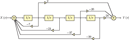
7.6.2 Cascade and parallel forms
Instead of simulating a system with the direct-form block diagram discussed in the previous section, it is also possible to express the system function as either the product or the sum of lower order sections, and base the block diagram on cascade or parallel combination smaller diagrams. Consider a system function of order M that can be expressed in the form
One method of simulating this system would be to build a diagram for each of the subsections Hi (s) using the direct-form approach discussed previously, and then to connect those sections in cascade as shown in Fig. 7.70.
An easy method of sectioning a system function in the style of Eqn. (7.238) would be to determine the poles and the zeros of the system function, and to use them for factoring numerator and denominator polynomials. Afterwards, each section may be constructed by using one of the poles. Each zero is incorporated into one of the sections, and some sections may have constant numerators. If some poles and zeros are complex-valued, we may choose to keep conjugate pairs together in second-order sections to avoid the need for complex gain factors in the diagram. The next example will illustrate this process.
Example 7.41: Cascade form block diagram
Develop a cascade form block diagram for simulating the system used in Example 7.40.
Solution: The system function specified in Example 7.40 can be factored into the form
The roots can be found easily using MATLAB (see MATLAB Exercise 7.3). Let us write H (s) as
by choosing
The cascade form simulation diagram is shown in Fig. 7.71.

It is also possible to consolidate the neighboring adders although this would cause the intermediate signals W1 (s) and W2 (s) to be lost. The resulting diagram is shown in Fig. 7.72.
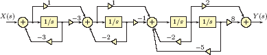
An alternative to the cascade form simulation diagram is a parallel form diagram which is based on writing the system function as a sum of lower-order functions:
A simulation diagram can be constructed by implementing each term in Eqn. (7.239) using the direct-form approach, and then connecting the resulting subsystems in a parallel configuration as shown in Fig. 7.73.

A rational system function H (s) can be sectioned in the form of Eqn. (7.239) using partial fraction expansion. If some poles and zeros are complex-valued, we may choose to keep conjugate pairs together in second-order sections to avoid the need for complex gain factors in the diagram. This process will be illustrated in the next example.
Example 7.42: Parallel form block diagram
Develop a parallel form block diagram for simulating the system used in Example 7.40.
Solution: The system function specified in Example 7.40 can be expanded into partial fractions as
Since the first two terms have complex poles and complex conjugate residues, we will combine them back into a second-order section to avoid the need for complex gain factors in the diagram. This results in
with
The parallel form simulation diagram is shown in Fig. 7.74.

7.7 Unilateral Laplace Transform
It was mentioned in earlier discussion that the Laplace transform as defined by Eqn. (7.1) is sometimes referred to as the bilateral Laplace transform.
An alternative version of the Laplace transform, known as the unilateral Laplace transform, is defined by
We use the subscript “u” to distinguish the unilateral Laplace transform from its bilateral counterpart. Comparing the definition in Eqn. (7.240) with the definition of the bilateral transform given by Eqn. (7.1) it is clear that the only difference is the lower limit of the integral. In fact, if the signal x (t) is causal, that is, if x (t) = 0 for t < 0, then both definitions of the Laplace transform produce the same result.
In many engineering applications we work with causal signals, and may not need to pay attention to which Laplace transform definition we use. On the other hand, for a non-causal signal, the two definitions produce different results. Consider a signal x (t) that is non-causal. The unilateral Laplace transform of x (t) is
Thus, the unilateral Laplace transform of a signal x (t) is the same as the bilateral Laplace transform of the signal [x (t) u (t)].
Because of the way Xu (s) is defined, its region of convergence is always to the right of a vertical line in the s-plane, and does not have to be explicitly stated. The ambiguity that we have observed with the bilateral Laplace transform in Eqns. (7.22) and (7.23) does not exist with the unilateral transform.
Most of the properties discussed in Section 7.3 for the bilateral Laplace transform apply to the unilateral Laplace transform as well. A few of the properties need to be modified, and a few new ones need to be introduced. These will be discussed briefly.
7.7.1 Time shifting
The use of the time shifting property with the unilateral Laplace transform requires special care. Recall the time shifting property derived in Eqn. (7.52) and repeated here:
Using Eqn. (7.242), the unilateral Laplace transform of x (t − τ) is
Correspondingly, the time shifting property will work for the unilateral Laplace transform only if the shift by τ does not cause any signal components to move from the negative time territory to positive time territory or vice versa. Mathematically we have the following:
Fig. 7.75 depicts a signal x (t) and three of its shifted versions. It can be shown that the time shifting property in Eqn. (7.244) holds for x1 (t) and x2 (t), but not for x3 (t).

(a) The signal x (t), (b) the signal xi (t) = x (t − 1), (c) the signal x2 (t) = x (t + 1), (d) the signal x3 (t) = x (ts + 2).
In contrast, the time shifting property does not hold for any amount of shift of the signal x (t) in Fig. 7.76 due to signal components that cross from left of the vertical axis to the right or vice versa.

(a) The signal x (t), (b) the signal x1 (t) = x (t − 1), (c) the signal x2 (t) = x (t + 1).
7.7.2 Differentiation in time
Given the transform pair
the following is also a valid transform pair
This property will be very important in using the unilateral Laplace transform for solving differential equations with initial conditions. The proof is similar to the proof of the corresponding property for the bilateral Laplace transform, and will be given here.
Proof: Using the Laplace transform definition in Eqn. (7.1), the transform of dx (t) /dt is
Integrating Eqn. (7.246) by parts yields
The term x (t) e−st must evaluate to zero for t → ∞ for the transform Xu (s) to exist. Therefore, Eqn. (7.247) reduces to
to complete the proof.
The unilateral Laplace transforms of higher-order derivatives can be found through repeated use of Eqn. (7.245). For example,
Using Eqn. (7.245) in Eqn. (7.249) yields
Similarly it can be shown that
and for the general case
As mentioned before, the primary utility of the unilateral Laplace transform is in solving differential equations with specified initial conditions. The next couple of examples will illustrate this.
Example 7.43: Using Laplace transform to solve a differential equation
Consider the circuit shown in Fig. 7.77(a) driven by the pulse signal shown in Fig. 7.77(b). Determine the output signal y (t) for t > 0 subject to the initial condition y (0+) = −2 V.
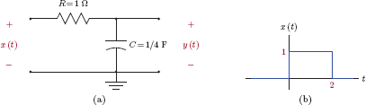
Solution: The system can be modeled with the following differential equation (see Example 2.9 in Chapter 2 for derivation):
Taking the unilateral Laplace transform of each side of the differential equation we obtain
The input signal x (t) can be written as
and its unilateral Laplace transform is
Using Eqn. (7.254) in Eqn. (7.253) and substituting the initial value y (0+) leads to
which can be written in the form
so that
and consequently
Using partial fraction expansion, we can write
The output signal is
and is shown in Fig. 7.78.
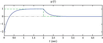
Software resources: |
Example 7.44: Solving second-order differential equation using Laplace transform
Find the solution of the second-order homogeneous differential equation
subject to initial conditions
Solution: Taking the unilateral Laplace transform of the differential equation leads to
Substituting initial conditions we obtain
which can be solved for Yu (s) to yield
The transform Yu (s) can be written in partial fraction form as
with residues
Therefore the solution is
The solution y(t) is shown in Fig. 7.79. It can easily be verified that y (t) satisfies the differential equation and the specified initial conditions.
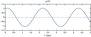
7.7.3 Initial and final value theorems
The initial value theorem is stated as follows:
Given the transform pair
we have
provided that the limit exists.
The initial value theorem does not apply to rational transforms in which the order of the numerator is equal to or greater than that of the denominator, since the limit in Eqn. (7.257) would not exist in that case.
The final value theorem is stated as follows:
Given the transform pair
we have
The final value theorem does not apply to a transform Xu (t) if the corresponding signal x (t) is unbounded, or if it has undamped oscillations. An unbounded signal indicates the presence of poles in the right half s-plane. Undamped oscillations are associated with poles on the jω axis of the s-plane other than at the origin s = 0. Consequently, the final value theorem should not be used with transforms that have poles on the jω axis or in the right half s-plane. A single pole at the origin s = 0 is permissible.
Example 7.45: Application of initial and final value theorems
Consider the transform
Can initial and final values be determined using initial and final value theorems?
Solution: Since the numerator order is lower than the denominator order, the initial value theorem can be used.
The final value theorem does not apply since Xu (s) has poles on the jω axis at s = ±j2. We may also recognize that Xu (s) is the Laplace transform of the signal
which does not have a final value due to the undamped oscillating term.
Example 7.46: Further exploring initial and final value theorems
Determine initial and final values of the signal with the Laplace transform
Solution: The numerator order is lower than the denominator order; therefore, the initial value theorem can be used.
The transform Xu (s) has a pair of complex conjugate poles at s = −2 ± j3 and a single pole at s = 0. Complex conjugate poles are in the left half s-plane. The single pole at the origin does not cause any problems in the use of the final value theorem since it is canceled by the factor s in Eqn. (7.258). The final value of x (t) is
7.5 Further Reading
[1] J. Bak and D.J. Newman. Complex Analysis. Undergraduate Texts in Mathematics. Springer, 2010.
[2] R.J. Beerends. Fourier and Laplace Transforms. Cambridge University Press, 2003.
[3] W.R.L. Page. Complex Variables and the Laplace Transform for Engineers. Dover Books on Electrical Engineering Series. Dover Publications, 1980.
[4] J.L. Schiff. The Laplace Transform: Theory and Applications. Springer Undergraduate Texts in Mathematics and Technology. Springer, 1999.
[5] J.L. Taylor. Complex Variables. Pure and Applied Undergraduate Texts. American Mathematical Society, 2011.
MATLAB Exercises
MATLAB Exercise 7.1: Three dimensional plot of Laplace transform
In Fig. 7.3 the magnitude of the transform
was graphed as a three-dimensional surface. In this exercise we will reproduce that figure using MATLAB, and display various cutouts of the Laplace transform surface on vertical lines s = σ + j0. The first step is to produce a set of complex values of s on a rectangular grid in the s-plane.
>> [sr,si] = meshgrid([-6:0.3:6] ,[-15:0.5:15]);
>> s = sr+j*si;
The next step is to compute the magnitude of the transform at each point on the grid. Additionally, values of magnitude that are greater than 2 will be clipped for graphing purposes.
>> Xs = @(s) (s+0.5)./((s+0.5).^2+4*pi*pi);
>> XsMag = abs(Xs(s));
>> XsMag = XsMag.*(XsMag<=2)+2.*(XsMag>2);
A three-dimensional mesh plot of X (s) can be generated with the following lines:
>> mesh(sr,si,XsMag);
>> axis([-6,6,-15,15]);
The script listed below produces a mesh plot complete with axis labels and color specifications.
1 % Script: matex_7_1a.m
2 %
3 [sr,si] = meshgrid([-6:0.3:6],[-15:0.5:15]);
4 s = sr+j*si;
5 Xs = @(s) (s+0.5)./((s+0.5).^2+4*pi*pi); % Eqn.(7.8)
6 XsMag = abs(Xs(s));
7 XsMag = XsMag,*(XsMag<=2)+2.*(XsMag>2);
8 shading interp; % Shading method: Interpolated
9 colormap copper; % Specify the color map used.
10 m1 = mesh(sr ,si , XsMag);
11 axis ([-6 ,6 ,-15 ,15]);
12 % Adjust transparency of surface lines.
13 set (m1 , ’ EdgeAlpha ’,0.6’,’ FaceAlpha ’ ,0.6);
14 % Specify x,y,z axis labels.
15 xlabel (’sigma’);
16 ylabel(’jomega’);
17 zlabel (’|X(s)|’);
18 % Specify viewing angles.
19 view(gca ,[23.5 ,38]);
In line 10 of the script, the handle returned by the function mesh(..) is assigned to the variable ml so that it can be used in line 13 for adjusting the transparency of the surface.
Alternatively, a contour plot of |X (s)| can be produced by slightly modifying the code. The script listed below gives a bird’s eye view of the magnitude of the transform by plotting points that have the same magnitude value as contours.
1% Script: matex_7_1b.m
2%
3 [sr,si] = meshgrid([-6:0.3:6],[-15:0.5:15]);
4 s = sr+j*si;
5 Xs = @(s) (s+0.5)./((s+0.5).~2+4*pi*pi); % Eqn.(7.8)
6 XsMag = abs(Xs(s));
7 XsMag = XsMag,*(XsMag<=2)+2.*(XsMag>2);
8 shading interp; % Shading method: Interpolated
9 colormap copper; % Specify the color map used.
10 values = [[0:0.04:0.2] ,[0.3:0.1:2]]; % z value for each contour.
11 m2 = contour (sr , si , XsMag , values) ; grid;
12 axis ([-6 ,6 ,-15 ,15]);
13 % Specify x,y axis labels.
14 xlabel (’sigma’);
15 ylabel (’jomega’);
The Fourier transform X (ω) is equal to the Laplace transform evaluated on the jω axis of the s-plane, that is,
Applying this relationship to the magnitudes of the two transforms, the magnitude of the Fourier transform is obtained by evaluating the magnitude of the Laplace transform on the jω axis. The script listed below demonstrates this.
1 % Script: matex_7_1c.m
2 %
3 [sr,si] = meshgrid([-6:0.3:6],[-15:0.5:15]);
4 s = sr+j*si;
5 Xs = @(s) (s+0.5)./((s+0.5).^2+4*pi*pi); % Eqn.(7.8)
6 XsMag = abs(Xs(s));
7 XsMag = XsMag,*(XsMag<=2)+2.*(XsMag>2);
8 % Define the trajectory s=j*omega
9 omega = [-15:0.01:15];
10 tr = j*omega;
11 % Produce a mesh plot and hold it.
12 shading interp;
13 colormap copper ;
14 m1 = mesh(sr ,si , XsMag);
15 hold on;
16 % Superimpose a plot of X(s) magnitude values evaluated on the
17 % trajectory using ’plot3’ function.
18 m2 = plot3(real(tr),imag(tr),abs(Xs(tr)), ’b-’,’LineWidth ’ ,1.5);
19 hold off ;
20 axis ([-6 ,6 ,-15 ,15]) ;
21 % Adjust transparency of surface lines.
22 set (m1 , ’EdgeAlpha’ ,0.6’, ’FaceAlpha’ ,0.6);
23 % Specify x,y,z axis labels.
24 xlabel (’sigma’);
25 ylabel (’jomega’);
26 zlabel (’|X(s)|’);
27 % Specify viewing angles.
28 view (gca ,[23.5 ,38]);
Lines 9 and 10 create a vector of s values on the jω axis. Line 18 graphs the values of |X (s)| along the jω axis using the plot3(..) function. It is also possible, with a few changes in the code, to cut the Laplace transform surface along the jω axis and display the profile of the cutout. The modified script to accomplish this is listed below:
1% Script: matex_7_1d.m
2%
3 [sr,si] = meshgrid([-6:0.3:6],[-15:0.5:15]);
4 s = sr+j*si;
5 Xs = @(s) (s+0.5)./((s+0.5).^2+4*pi*pi); % Eqn.(7.8)
6 XsMag = abs(Xs(s));
7 XsMag = XsMag,*(XsMag<=2)+2.*(XsMag>2);
8 % Define the trajectory s=j*omega
9 omega = [-15:0.01:15];
10 tr = j*omega;
11 % Produce a mesh plot and hold it.
12 shading interp;
13 colormap copper ;
14 % Set the surface equal to zero in the right half of the s-plane.
15 XsMag = XsMag .*(sr <=0);
16 m1 = mesh(sr ,si , XsMag);
17 hold on;
18 % Superimpose a plot of X(s) magnitude values evaluated on the
19 % trajectory using ’plot3’ function.
20 m2 = plot3(real(tr),imag(tr),abs(Xs(tr)), ’b-’,’LineWidth ’ ,1.5);
21 % Stem plot on the trajectory for a painted profile look.
22 m3 = stem3(real(tr([1:25:3000])) ,imag(tr([1:25:3000])) ,
23 abs(Xs(tr([1:25:3000]))));
24 hold off;
25 axis ([-6 ,6 ,-15 ,15]) ;
26 % Adjust transparency of surface lines.
27 set (m1 , ’ EdgeAlpha ’ ,0.6’, ’ FaceAlpha ’ ,0.6);
28 % Adjust color of cutout profile.
29 set(m3 , ’Marker’,’none’,’Color’ ,[0.01,0.74,0.25]);
30 % Specify x,y,z axis labels.
31 xlabel (’sigma’);
32 ylabel (’jomega’);
33 zlabel (’|X(s)|’);
34 % Specify viewing angles.
35 view(gca ,[23.5 ,38]);
Notice how the magnitude values in the right half of the s-plane are suppressed in line 15.
Software resources:
matex_7_la.m
matex_7_lb.m
matex_7_lc.m
matex_7_ld.m
MATLAB Exercise 7.2: Computing the Fourier transform from the Laplace transform
The Fourier transform of a signal is equal to its Laplace transform evaluated on the jω-axis of the s-plane.
Consider the Laplace transform
The first method of computing and graphing the Fourier transform of the signal is to use an anonymous function for X (s) and evaluate it on the jω-axis. The magnitude |X (ω) | is graphed using the following statements:
>> Xs = @(s) (s+0.5)./((s+0.5).^2+4*pi*pi);
>> omg = [-15:0.05:15];
>> Xomg = Xs(j*omg);
>> plot(omg,abs(Xomg)); grid;
If the phase is needed, it can be graphed using
>> plot(omg,angle(Xomg)); grid;
The second method is to use MATLAB function freqs(..). We will begin by writing X (s) in rational form with numerator and denominator polynomials ordered in descending powers of s.
Vectors “num” and “den” to hold numerator and denominator coefficients should be entered as
>> num = [1,0.5];
>> den = [1,1 ,39.7284];
Afterwards the magnitude and the phase of the Fourier transform may be computed and graphed with the statements
>> omg = [-15:0.05:15];
>> Xomg = freqs(num,den,omg);
>> plot(omg,abs(Xomg),’r’); grid;
>> plot(omg,angle(Xomg), ’r’); grid;
Software resources:
matex_7_2a.m
matex_7_2b.m
MATLAB Exercise 7.3: Graphing poles and zeros
Consider a CTLTI system described by the system function
Poles and zeros of the system function can be graphed on the s-plane by entering coefficients of numerator and denominator polynomials as vectors and then computing the roots.
>> num = [1,-1,-4,4];
>> den = [1 ,7 ,21 ,37 ,30];
>> z = roots(num);
>> p = roots(den);
To produce the graph we need
>> plot(real(z),imag(z), ’o’,real(p),imag(p),’x’);
which uses “o” for a zero and “x” for a pole. The graph produced does not display the real and imaginary axes in the s-plane. A more complete pole-zero plot may be generated with the following lines:
 >> plot(real(z),imag(z), ’o’,real(p),imag(p),’x’ ,...
   [-3, 3],[0,0],’k:’ , [0,0], [-3,3], ’k:’);
>> xlabel(’sigma’);
>> ylabel(’jomega’);
Software resources:
matex_7_3.m
MATLAB Exercise 7.4: Residue calculations
Consider the transform
In expanding X (s) to partial fractions, MATLAB function residue(..) can be used. Numerator and denominator polynomials are specified by means of two vectors that list the coefficients of these polynomials in the order of descending powers of s.
>> num = conv([1,0],[1,-2]);
>> den = [1 ,9 ,30 ,42 ,20];
>> [res,poles,qt] = residue(num,den)
res =
1.7000 - 1.9000 i
1.7000 + 1.9000 i
-4.0000
0.6000
poles =
-3.0000 +1.0000i
-3.0000 - 1.0000i
-2.0000
-1.0000
qt =
[]
Notice how the convolution function conv(..) is used for multiplying the numerator factors s and (s − 2) expressed through the vectors [1,0] and [1, −2] respectively. Returned vectors “res” and “poles” hold the residues and the poles of the partial fraction expansion. The vector “qt” is empty since the numerator order is less than the denominator order in this case. The order of residues and poles in these two vectors is important. We have
The partial fraction expansion we seek is in the form
Consider another transform
the residues for which can be computed through
>> num = [3,2,5];
>> den = [1 ,4 ,20];
>> [res,poles,qt] = residue(num,den)
res =
-5.0000 + 4.3750 i
-5.0000 - 4.3750 i
poles =
-2.0000 + 4.0000 i
-2.0000 - 4.0000 i
qt =
3
The vector “qt” has a single element, and corresponds to the quotient polynomial Q (s) = 3. The partial fraction expansion for X2 (s) is
matex_7_4a.m
matex_7_4b.m
MATLAB Exercise 7.5: Symbolic calculations for Laplace transform
It is also possible to do symbolic processing with MATLAB. As a first step we need to specify that “s” and “t” are symbolic variables rather than numeric variables. This is accomplished with the statement
>> syms s t
Notice that there is no comma, but rather just space, separating the two symbolic variables. The next step is to define the signal x (t) the Laplace transform of which we seek. For example, the signal
is defined with the statement
>> xt = exp(-t)*cos (2*t);
The resulting variable “xt” is also a symbolic variable since it utilizes “t” defined with the previous statement. The Laplace transform can be computed using the function laplace(..).
>> Xs = laplace(xt)
Xs =
(s + 1)/((s + 1)^2 + 4)
MATLAB returns the answer as a symbolic expression. To display the answer in a way closer to its natural form, use
>> pretty(Xs)
s + 1
------------
2
(s + 1) + 4
which corresponds to
Combining the statements listed above, the transform can be computed in a compact form as
>> syms s t;
>> Xs = laplace(exp(-t)*cos (2*t));
Some observations:
In using the function laplace(..) with just one argument we assume that the independent variable of the signal is named “t” and the independent variable of the transform is named “s”. If, for some reason, the names “v” and “w” need to be used in place of “t” and “s” respectively, then an alternative syntax of the function with three arguments can be employed:
>> Xs = laplace(xt,v,w)
The function iapiace(..) computes the Laplace transform integral starting with the lower limit t = 0. In other words, the transform computed is the unilateral Laplace transform discussed in Section 7.7.
Inverse Laplace transform can be computed symbolically using the function iiapiace(..). Consider the problem of finding the inverse Laplace transform of
which was solved in Example 7.22 through the use of partial fractions. The following set of statements produce the solution using symbolic processing in MATLAB:
>> syms s t
>> Xs = (s+1)/(s*(s+2));
>> xt = ilaplace(Xs)
xt =
1/(2* exp (2*t)) + 1/2
>> pretty(xt)
1 1
---------- + -
2 exp(2 t) 2
The result displayed corresponds to
The symbolic result obtained for the signal x (t) can be graphed using the function ezplot (..) as follows:
>> ezplot(xt,[0 ,5]); grid;
>> axis([0,5 ,0 ,1.2]);
The graph produced is shown in Fig. 7.80.

Software resources:
matex_7_5a.m
matex_7_5b.m
MATLAB Exercise 7.6: Computing frequency response of a system from pole-zero layout
The problem of obtaining the frequency response of a CTLTI system from the placement of its poles and zeros in the s-domain was discussed in Section 7.5.5. In this exercise we will use MATLAB to compute the frequency response for a system characterized by the system function
The system has one zero at s = 1 and one pole at s = −2. Suppose we need the frequency response of this system at the frequency ω = 3 rad/s, which is equal to the system function evaluated for s = j3:
Using vector notation
where we have defined the vectors and for notational convenience. The script listed below computes the vectors and and uses them for computing the magnitude and the phase of the system function at ω = 3 rad/s:
1 % Script: matex_7_6a.m
2 %
3 omega = 3;
4 s = j*omega;
5 B = s-1;
6 A = s+2;
7 mag = abs(B)/abs(A);
8 phs = angle(B)-angle(A);
This script computes the frequency response of the system at one specific frequency. It would be more interesting if we could use the same idea to compute the frequency response of the system at a large number of frequencies so that its magnitude and phase can be graphed as functions of w. Let us change the variable “omega” into a vector by editing line 1 of the script:
1 omega = [-5:0.01:5];
This change causes the variable “s” to become a complex vector with 1001 elements. Also, in line 5, the standard division operator “/” needs to be changed to the element-by-element division operator “./” to read
5 mag = abs(B)./abs(A);
The MATLAB script is listed below with these modifications and the addition of graphing statements:
1 % Script: matex_7_6b.m
2%
3 omega = [-5:0.01:5];
4 s = j*omega;
5 B = s-1;
6 A = s+2;
7 mag = abs(B)./abs(A);
8 phs = angle(B)-angle(A);
9 clf ;
10 subplot (2,1,1);
11 plot (omega , mag);
12 title(’Magnitude of the frequency response’);
13 xlabel(’omega (rad/s)’); grid;
14 subplot (2,1,2);
15 plot (omega , phs);
16 title(’Phase of the frequency response’);
17 xlabel(’omega (rad/s)’); grid;
Software resources:
matex_7_6a.m
matex_7_6b.m
MATLAB Exercise 7.7: Frequency response from pole-zero layout revisited
In MATLAB Exercise 7.6 we have explored a method of computing the frequency response of a CTLTI system based on the graphical interpretation of the pole-zero layout of the system function, discussed in Section 7.5.5. The idea can be generalized into the development of a MATLAB function ss_freqs(..) for computing the frequency response.
1 function [mag,phs] = ss_freqs(zrs,pls,gain,omega)
2 nz = length(zrs); % Number of zeros.
3 np = length(pls); % Number of poles.
4 nomg = length(omega); % Number of frequency points.
5 s = j*omega; % Get points on the imaginary axis.
6 mag = ones(1,nomg);
7 phs = zeros(1,nomg);
8 if (nz > 0) ,
9 for n = 1: nz
10 mag = mag .* abs (s-zrs (n));
11 phs = phs +angle (s-zrs (n));
12 end;
13 end;
14 if (np > 0) ,
15 for n = 1: np
16 mag = mag ./abs (s-pls (n));
17 phs = phs - angle (s-pls (n));
18 end;
19 end;
20 mag = mag*gain;
21 phs = wrapToPi (phs);
Line 21 of the function causes phase angles to be contained in the interval (-n,n). The script listed below may be used for testing ss_freqs (..) with the system function
1 % Script: matex_7_7.m
2 %
3 num = [1,0.5];
4 den = [1,1 ,39.7284];
5 zrs = roots(num); % Compute zeros .
6 pls = roots(den); % Compute poles.
7 omg = [-15:0.05:15]; % Vector of frequencies.
8 [mag,phs] = ss_freqs(zrs,pls,1,omg);
9 clf ;
10 subplot (2,1,1) ;
11 plot (omg ,mag); grid;
12 xlabel(’omega (rad/s)’);
13 subplot (2,1,2);
14 plot (omg ,phs); grid;
15 xlabel(’omega (rad/s)’);
Software resources:
ss_freqs.m
matex_7_7.m
MATLAB Exercise 7.8: System objects
MATLAB has some functions that create and work with objects to represent linear and time-invariant systems. Consider, for example, a CTLTI system described by the system function
An object named “sysl” representing this system can be created in MATLAB with the following lines:
>> num = [1,0,1];
>> den = [1 ,5,17 ,13];
>> sys1 = tf(num,den)
Transfer function:
s ^ 2 + 1
-----------------------
s^3 + 5 s^2 + 17 s + 13
The object “sysl” created with a call to the function tf(..) may be used with other functions that accept system objects. For example, a pole-zero plot can be generated through
>> pzmap(sys1)
The impulse response of the system may be graphed using the following code:
>> t = [0:0.01:5];
>> h = impulse(sys1,t);
>> plot(t,h); grid;
Similarly, the unit-step response is graphed using
>> t = [0:0.01:5];
>> y = step(sys1 ,t);
>> plot(t,y); grid;
A system can be specified in a variety of ways. An alternative to using the numerator and the denominator coefficients is to use the zeros and the poles of the system through the function zpk(..). For example, an object “sys2” for the system function
is created by
>> zrs = [0,1];
>> pls = [1,2,3];
>> sys2 = zpk(zrs,pls ,10)
Let the input signal to this system be
The response of the system may be computed and graphed with the following code:
>> t = [0:0.01:3];
>> x = cos(2*pi*2*t);
>> [y,t] = lsim(sys2,x,t);
>> plot(t,x,t,y);
Software resources:
matex_7_8a.m
matex_7_8b.m
matex_7_8c.m
MATLAB Exercise 7.9: Bode plots
Construct a Bode plot for the system with system function
Solution: The easiest method is to use system objects. The following code accomplishes this
>> zrs = [0,1];
>> pls = [-1,-2,-3];
>> sys = zpk(zrs,pls ,10);
>> bode(sys); grid;
Software resources:
matex_7_9.m
MATLAB Exercise 7.10: Solving a differential equation through Laplace transform
Two examples of using the unilateral Laplace transform for solving differential equations with specified initial conditions were given in Section 7.7. In this exercise we will explore the use of symbolic processing capabilities of MATLAB for solving similar problems. The functions laplace(..) and ilaplace(..) were explored in MATLAB Exercise 7.5. They compute the forward and the inverse Laplace transform with the assumption that the time-domain signal involved is causal. In effect they implement the unilateral variant of the Laplace transform.
Consider the RC circuit problem solved in Example 7.43. The governing differential equation is
with the initial value of the solution specified as y (0+) = −2 V. The input signal is a unit amplitude pulse with a duration of 2 seconds.
The following script can be used for solving the problem and graphing the result:
1 % Script: matex_7_10.m %
2 %
3 syms s t Ys
4 xt = heaviside(t)-heaviside(t-2); % x(t)=u(t)-u(t-2)
5 Xs = laplace(xt); % Laplace transform of x(t)
6 Y1 = s*Ys+2; % Laplace transform of dy/dt
7 Ys = solve(Y1+4*Ys-4*Xs % Solve for Y(s)
8 yt = ilaplace(Ys); % Inverse Laplace transform of Y(s)
9 ezplot(yt ,[0 ,5]); grid;
10 axis([0,5,-2.5,1.5]);
In line 3 we declare three symbolic variables. The variable “Ys” corresponds to the yet unknown transform Yu (s). In line 4 the input signal is specified in symbolic form. Note that we make use of the symbolic function heaviside(..) to represent the unit-step function. The symbolic result “Y1” represents the Laplace transform
Line 7 of the script uses the function solve (..) to solve the equation
for Yu (s). The graph produced by the function ezplot(..) on line 9 should match Fig. 7.78.
Software resources:
matex_7_10.m
Problems
7.1. Using the Laplace transform definition given by Eqn. (7.1) determine the transform of each signal listed below. For each transform construct a pole-zero diagram and specify the ROC.
- x (t)= e−2t u (t)
- x (t)= e−2t u (t − 1)
- x (t) = e2t u (−t)
- x (t) = e2t u (−t + 1)
7.2. Using the Laplace transform definition given by Eqn. (7.1) determine the transform of the signal
where a > 0 and t > 0. Put the transform into a closed form using the appropriate formula. Afterwards construct a pole-zero plot and indicate the ROC.
7.3. Pole-zero diagrams for four transforms are shown in Fig. P.7.3. For each, determine the ROC if it is known that the Fourier transform of x (t) exists.
7.4. Consider again the four transforms with pole-zero diagrams shown in Fig. P.7.3. Determine the ROC for each of the transforms if x (t) is known to be causal in each case.
7.5. Repeat Problem 7.3 if x (t) is known to be anti-causal for each case.
7.6. The Laplace transform of a signal x (t) is given by
Which of the following Fourier transforms can be obtained from X (s) without actually determining the signal x (t)? In each case, either determine the indicated Fourier transform or explain why it cannot be determined.
ℱ{xt)}
ℱ{xt) et}
ℱ{xt) e−3t}
7.7. The Laplace transform of a signal x (t) is given by
Which of the following Fourier transforms can be obtained from X (s) without actually determining the signal x (t)? In each case, either determine the indicated Fourier transform or explain why it cannot be determined.
7.8. Construct a pole-zero diagram and specify the ROC for each of the transforms given below. Also, determine the Fourier transform X (ω) if it exists.
7.9. Using the linearity property of the Laplace transform, determine X (s) for each of the signals listed below. Also indicate the ROC in each case.
x (t) = 3 e−t u (t) − 5 e−3t u (t)
x (t) = 3 e−t u (t) + 2 e3t u (−t)
x (t) = 5 (t) + 2 e−t u (t)
x (t) = (1 − e−t) u (t)
x (t) = cos (2t) u (t) + 2 sin (3t) u (t)
x (t) = e−2t cos (3t) u (t)
7.10. Using time shifting and linearity properties of the Laplace transform as needed, determine X (s) for each of the signals listed below. Also indicate the ROC in each case.
x (t) = e−2(t−1) u (t − 1)
x (t) = e−2t u (t − 1)
x (t) = e2(t+1) u (−t − 1)
x (t) = e2t u (−t − 1)
x (t) = e2t u (−t + 1)
7.11. Determine the Laplace transform of the signal
using two different methods as specified below. Show that the same result can be obtained through each.
Use a trigonometric identity to express x (t) as the sum of a cosine and a sine term. Afterwards use the entries for cos (3t) and sin (3t) from the Laplace transform table.
Use Euler’s formula to express x (t) as a sum of complex exponentials. Afterwards use the entry for eat from the Laplace transform table.
7.12. Determine the Laplace transform of each signal listed below. Specify the ROC in each case. Sketch each signal and justify the ROC based on the characteristics of each signal.
7.13. Using the linearity and time shifting properties, determine the Laplace transform of each signal shown graphically in Fig. P.7.13. Specify the ROC in each case.
7.14. Express each of the signals shown in Fig. P.7.14 in terms of the unit-ramp function and its scaled and/or time shifted versions. Afterwards, determine the Laplace transform of each signal using linearity and time shifting properties, Specify the ROC in each case.
7.15. The signal x (t) is in the form of one cycle of a sinusoidal waveform as shown in Fig. P.7.15.
Determine its Laplace transform using two different methods:
Apply Laplace transform definition directly. Hint: Express the sinusoidal signal using Euler’s formula.
Use the transform for x1 (t) = sin (ω0t) u (t) and then apply linearity and time shifting properties.
7.16. The transforms given below correspond to causal signals. Using the table of Laplace transforms, determine the inverse Laplace transform of each.
Hint: For each case find a similar entry in the table and adjust its parameters to obtain the desired result.
7.17. Determine the inverse Laplace transform of each function listed below using partial fraction expansion.
7.18. Use partial fraction expansion to find the inverse Laplace transform of each function listed below.
-
Construct a pole-zero diagram for X (s).
List all possibilities for the ROC.
For each choice of the ROC listed in part (b) determine the inverse transform x (t), and indicate whether it is square integrable or not.
7.20. For each Laplace transform given below, find all possible signals that might have led to that transform.
7.21. Use partial fraction expansion and the time shifting property to find the inverse Laplace transforms of functions listed below. Assume each transform corresponds to a causal signal.
7.22. Find a system function for each CTLTI system described below by means of a differential equation.
7.23. Find a differential equation for each CTLTI system described below by means of a system function.
7.24. Let yu (t) represent the response of a CTLTI system to a unit-step input signal x (t) = u (t). Determine the system function for each system the unit-step response of which is given below. Afterwards find a differential equation for each system.
yu (t) = e−t u (t)
yu (t) = (1 − e−t) u(t)
yu (t)= (e−t − e−2t) u (t)
yu (t)=(1 − e−t + 2 e−2t) u (t)
yu (t) = [1 − 0.3 e−t cos (2t)] u (t)
7.25. Let yr (t) represent the response of a CTLTI system to a unit-ramp input signal x (t) = tu(t). Determine the system function for each system the unit-step response of which is given below. Afterwards find a differential equation for each system.
yr (t) = (1 − e−t) u (t)
yr (t) = (e−t + 2 e−2t − 4 e−3t) u (t)
yr (t) = [1 − 0.3 e−t cos (2t)] u (t)
7.26. A CTLTI system is described by means of the system function
Determine the response of the system to the following signals:
x (t) = e−0.5t
x (t) = e(−0.5+j2)t
x(t) = ej3t
x (t) = e−j3t + ej3t
x (t) = ej2t + ej3t
7.27. Show that, for a CTLTI system with a real-valued impulse response, the value of the system function at the point is the complex conjugate of its value at the point s = s0. Given
where
and
prove that
Hint: Use the Laplace transform definition with the impulse response h (t) and evaluate the result at . Manipulate the resulting expression to obtain the desired proof.
7.28. A CTLTI system is described by means of the system function
Determine the response of the system to the following signals:
x (t) = cos (2t)
x (t) = e−0.5t cos (2t)
x (t) = e−t sin (2t)
7.29. A CTLTI system has the impulse response
Using Laplace transform techniques, determine the response of the system to each input signal listed below. Identify transient and steady-state components of the output signal in each case.
7.30. Determine the impulse response of each system specified below by means of a system function.
7.31. Consider again the system used in Problem 7.29. Using the Laplace transform, determine the response of the system to the signal
which is similar to the input signal in part (a) of Problem 7.29 except it exists for all t instead of being turned on at t = 0. Compare the output signal to that obtained in Problem 7.29(a) and comment on the result.
7.32. A CTLTI system has the impulse response
Using Laplace transform techniques, determine the response of the system to the input signal x (t) = e−0.5t cos (2t) u (t).
7.33. Construct a pole-zero diagram for each of the system functions given below.
7.34. Pole-zero diagrams for four system functions are shown in Fig. P.7.34. For each, determine the the system function H (s). Set |H (0)| = 1 for each system.
7.35. For each system function given below, sketch the magnitude and phase characteristics using the graphical method outlined in Section 7.5.5.
7.36. The system functions given below correspond to causal systems. For each system, construct a pole-zero plot and determine whether the system is stable or not.
7.37. Determine which of the system functions given below could represent a system that is both causal and stable.
7.38. A causal system is described by the differential equation
7.39. Consider a first-order allpass system with system function
Compute and sketch the phase response of this system.
Determine the response y (t) of the system to the input signal x (t) = e−t u (t).
Find analytical expressions for the magnitude responses X (ω) and Y (ω) of the input and the output signals.
Sketch each magnitude spectrum.
7.40. Repeat Problem 7.39 using the second-order allpass system with the system function
7.41. A CTLTI system has the system function
Does the system have an inverse that is both causal and stable?
Express the system function in the form of the product of two system functions
such that H1 (s) corresponds to a minimum-phase system and H2 (s) corresponds to a first-order allpass system.
Find the inverse system . Is it causal? Is it stable?
Find the overall system function of the cascade combination of H (s) and .
7.42. For each CTLTI system defined by means of a differential equation below, determine whether a causal and stable inverse exists. If the answer is yes, find a differential equation for the inverse system.
7.43. Refer to the Bode magnitude plot in Example 7.39.
Show that the value of the asymptote for the Bode magnitude plot is 13.98 dB at ω = 5 rad/s.
Also show that, at ω = 300 rad/s, the corner of the asymptote is at −3.52 dB.
7.44. Develop a direct-form block diagram for each system specified below by means of a system function. Assume that each system is causal and initially relaxed.
7.45. Develop a cascade-form block diagram for each system specified below by means of a system function. Assume that each system is causal and initially relaxed. Use first- and second-order cascade sections and ensure that all coefficients are real.
7.46. Develop a parallel-form block diagram for each system specified in Problem 7.45. Assume that each system is causal and initially relaxed. Use first- and second-order parallel sections and ensure that all coefficients are real.
7.47. Let Xu (s) be the unilateral Laplace transform of the signal x (t), that is
For each of the signals listed below, write the unilateral Laplace transform Gu (s) in terms of Xu (s). In each case, indicate the condition for obtaining the transform directly from Xu (s) without having to find x (t) first.
g (t) = x (t − 1)
g (t) = x (t + 2)
g (t) = x (2t)
g (t) = e−2t x (t)
g (t) = tx (t)
7.48. For the RLC circuit shown in Fig. P.7.48, the initial values are
7.49. For the circuit shown in Fig. P7.49, the initial values are
Find a differential equation between the input x (t) and the output y (t).
Obtain the system function H (s) from the differential equation found in part (a).
Using unilateral Laplace transform determine the output signal if x (t) = u (t).
Determine the output signal if x (t) = e−t u (t).

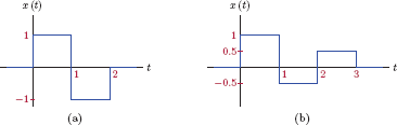
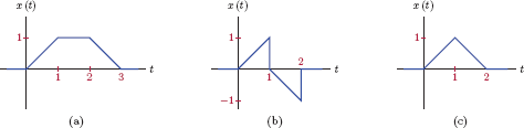
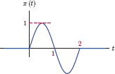


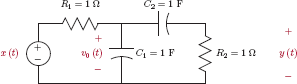
MATLAB Problems
-
Determine the poles and zeros of X (s). Manually construct a pole-zero diagram.
Write a MATLAB script to evaluate the magnitude of X (s) at a grid of complex points in the s-plane. Use the function meshgrid(..) to generate the grid of complex points within the ranges −5 < σ < 5 and −5 < ω < 5 with increments of 0.1 in each direction.
Use the function mesh(..) to produce a three dimensional mesh plot of |X (s)|.
Evaluate the Laplace transform for s = jω and use the function piot3(..) to plot it over the three-dimensional mesh plot.
7.51. Refer to Problem 7.8. Using MATLAB, construct a pole-zero plot for each transform listed.
7.52. Refer to Problem 7.8. For each signal that has a Fourier transform, write a script to compute X (ω) from the Laplace transform X (s) given, and to graph it in the frequency range −10 ≤ ω ≤ 10 rad/s.
7.53. Each transform given below corresponds to a causal signal x (t). Use symbolic mathematics capabilities of MATLAB to find the inverse Laplace transform of each. Refer to MATLAB Exercise 7.5 for an example of the solution technique.
7.54. A CTLTI system is described by means of the system function
Compute and graph the response of the system to the signal
using the following steps:
Define a system object “sys” for H (s).
Create a vector with samples of the input signal.
Use the function isim(..) to compute the output signal.
7.55. Using the function residue(..) obtain a partial fraction expansion for the transform X (s) given by
Use the results from MATLAB to write X(s) in partial fraction format.
7.56. Using system objects and the function bode(..), construct Bode magnitude and phase plots for the system functions given below:
7.57. Consider the second-order system function
Let ω0 = 5 rad/s. Using system objects and the function bode(..), construct Bode magnitude and phase plots for the system for ζ = 0.01, 0.1, 0.5, 1, 2.
7.58. Refer to Problem 7.41.
Using system objects of MATLAB, construct objects to represent H (s), H1 (s) and .
Compute and graph the frequency responses (magnitude and phase) for H (s), H1 (s), and .
Compute and graph the unit-step responses of H (s) and . Comment on the results.
7.59. Refer to the RLC circuit in Problem 7.48. Using symbolic mathematics capabilities of MATLAB, write a script to compute and graph the response of the circuit for the input signal and the initial conditions specified in the problem statement. Use MATLAB Exercise 7.10 for an example of the solution technique.
7.60. Refer to the RLC circuit in Problem 7.49. Using symbolic mathematics capabilities of MATLAB, write a script to compute and graph the response of the circuit for the input signal and the initial conditions specified in the problem statement. Use MATLAB Exercise 7.10 for an example of the solution technique.
MATLAB Projects
7.61. Consider the second-order system analyzed in Section 7.5.10. Its system function is
Let y (t) be the unit-step response of this system.
Determine the Laplace transform of the unit-step response y (t). Afterwards use the final value theorem to verify that the final value of the unit-step response is unity.
Develop a MATLAB script to compute the unit-step response of this system. Construct a system object for specified values of parameters ω0 and ζ. Use the function step(..) to compute the step response for 0 ≤ t ≤ 30 s with increments of T = 0.01 s.
One performance measure of the responsiveness of a system is the rise time which is defined as the time it takes for the unit-step response to progress from 10 percent to 90 percent of its final value. Investigate the dependency of the rise time (tr) on parameter ζ. Set ω0 = 1 rad/s, and use the script from part (b) repeatedly with varying values of ζ. Measure the rise time from the graph and/or the data vector for each ζ value. Roughly sketch the relationship between tr and ζ.
7.62. Refer to Problem 7.61. Another performance measure for a system is the settling time which is defined as the time it takes for the unit-step response to settle within a certain percentage of its final value. Let ts represent the 5 percent settling time, that is, the time it takes for the response to settle in the interval 0.95 < y (t) < 1.05 and stay. Using the MATLAB script developed in Problem 7.61 investigate the dependency of the settling time on parameter ζ. Use ω0 = 1 rad/s. Roughly sketch the relationship between ts and ζ.
1 Care must be taken in certain circumstances. If the time shift makes a causal signal non-causal then the points s = ∞ + jω would need to be excluded from the ROC. Similarly, if an anti-causal signal loses its anti-causal property as the result of a shift, then the points s = −∞ + jω need to be excluded.
2 One decade corresponds to a tenfold change in ω. If ω2 = 10ω1, then .