After having modelled individual claim sizes and the number of claims, the next step is now to aggregate the individual claims and determine the resulting distribution. Even if the claim sizes are assumed to be independent (and independent of the number of claims), this is already a challenging yet classical actuarial task. In this chapter we will review the main techniques available for this purpose and then also discuss implications for the methods under reinsurance. Section 6.6 then gives some numerical illustrations and in Section 6.7 we will discuss some general aspects of the aggregation of dependent risks.

6.1 General Formulas for Aggregating Independent Risks

For most of this chapter we will assume that the two processes {N(t);t ≥ 0} and are independent. Recall from Chapter 2 that the total or aggregate claim amount at time t is defined by

Under the independence assumption, its c.d.f. then is

(6.1.1)

Whereas (6.1.1) fully specifies the total claim distribution, in this form it is not a workable expression to numerically evaluate F_S(t) and we typically will have to look for ways to approximate F_S(t). Since convolutions can efficiently be handled by Laplace transforms, a first step to simplify the expression is to look at the Laplace transform of S(t):

(6.1.2)

where Q_t(z) is the generating function of the number of claims. From this expression one now obtains general formulas for the first few moments of S(t).

• The most essential quantity related to the total claim amount is its expected value. As a function of time it offers a global picture of what happens to the portfolio over time. Taking the derivative with respect to s at s = 0 in (6.1.2) one easily obtains
  (6.1.3)
  for the mean total claim amount. This expression illustrates the complementary role of the average claim size and the average claim number. Clearly, this formula is pleasant and helpful when pricing according to the expected value principle, as dealing with the claim sizes and claim frequency can be separated.
• For the variance, Faa di Bruno’s formula entails
  (6.1.4)
  The role of the two ingredients comes out even better if we look at the dispersion. It easily follows from the above that
  
  This illustrates that the variability is not only caused by the variability in claim sizes but also by that in the claim numbers. The above expression is useful in premium calculations that are based on the first two moments of S(t) (cf. Chapter 7).
• Higher‐order moments of S can be derived by taking the respective higher‐order derivatives of at s = 0. In general, the nth moment of S can be expressed through combinations of the first n moments of X and of N.

Note that for the special case of a homogeneous Poisson process Ñ_λ, one obtains

and more generally for the nth cumulant of S(t). The simplicity of these formulas is reason for the popularity of the compound Poisson model.¹

Another general property of the total claim amount shows its direct dependence on the claim size distribution. Since a sum of non‐negative random variables is always larger than the largest element in the sum, we note that and hence

Letting we notice that

The above relation shows how the tail behavior of the total claim amount crucially depends on the heaviness of the individual claim size distribution and on the expected number of claims.

6.2 Classical Approximations for the Total Claim Size

A useful aggregate claim approximation should give reasonably accurate estimates and at the same time clarify the specific role of the two ingredients, the claim size and the claim number. We will now deal with several approximations for F_S(t) that have been used in this context. In Section 6.6 we will implement these methods in R and compare their performance.

6.2.1 Approximations based on the First Few Moments

If the number of claims is large (which may be due to large t), then one can expect that for the sum of independent random variables, in case of finite variance Var(X), a central limit effect will be dominant. The normal approximation

(6.2.5)

may then be feasible. For this approximation to be useful, the number of terms in the sum should indeed be large, and it has to be the larger, the more skewed the distribution of the individual risks X_i is. Whereas this may work sufficiently well for large time horizons, within the typical one‐year timeframe and appropriate choice of F_X, approximation (6.2.5) is usually too coarse in the regions of interest. If the skewness coefficient ν_S(t) is available, then a classical correction of (6.2.5) is the normal‐power approximation

(6.2.6)

for z ≥ 1.

Alternatively, if the first three moments of S = S(t) are available, it has also been suggested that S can be approximated by a shifted gamma distribution with the same first three moments, that is,

Clearly, this can only be done if the skewness coefficient ν_S is positive.

Whenever there are higher moments available, one can use the rather elegant theory of orthogonal polynomial expansions to improve the approximation. For that purpose, starting from a reference density function f_r(x) (defined on interval I) which one suspects to already be a reasonable approximation for the density f_S(x) of the aggregate claim distribution, one adds correction terms based on moments of S. Concretely, if all moments for f_r exist, then the Gram–Schmidt orthogonalization identifies a set (π_i)_i≥0, where π_i is a polynomial of degree i, for which

(6.2.7)

If for some α > 0, then this set of orthonormal polynomials is complete in the respective L² space, and hence if , one can express f_S(x)/f_r(x) as , where

If K moments of S are available, one can correspondingly determine coefficients A₀, …, A_K and approximate f_S by

If the reference density f_r has m parameters, one can choose them in such a way that the first m moments corresponding to f_r coincide with those of S(t). Let us consider two concrete examples:

• If we want to improve the normal approximation above, we can choose f_r(x) to be the density of a normal random variable. Here and the resulting polynomial family is
  
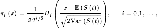
  where H_i(x) = ϕ⁽ⁱ⁾(x)/ϕ(x) are the Hermite polynomials, with ϕ(x) denoting the density of the standard normal distribution. This is also known as the Gram–Charlier approximation. If we have (estimates for) the skewness ν_S(t) and the excess kurtosis of S(t) available, the resulting approximation is
  (6.2.8)
  where . That is, we get a refinement of (6.2.5) using the third and fourth moment. The three terms of (6.2.8) in fact coincide with the first three terms of the so‐called Edgeworth expansion, which builds on saddlepoint approximations and also enjoys some popularity in actuarial circles.
• Choosing f_r(x) to be a gamma(α, β) density, one can improve on the gamma approximation for S(t). Here and the respective orthogonal polynomial family is
  
  where denote the generalized Laguerre polynomials. Furthermore and . By construction, again A₁ = A₂ = 0. The resulting approximation is referred to as Bower’s gamma approximation. Observe that if we truncate the approximation after K terms, the tail of f_S(t) is approximated by the dominant order x^Kf_{Γ(α, β)}(x), which is itself a gamma‐type decay. It will turn out that such a tail behavior is in fact quite appropriate under rather general conditions (cf. Section 6.2.2).
• For situations with heavy tails, it is tempting to choose a heavy‐tailed reference density f_r and then improve the approximation of S(t) with higher moments according to the recipe above. For a log‐normal density f_r, the corresponding family of orthonormal polynomials has recently been worked out in Asmussen et al. [60]. Note, however, that the resulting family is not complete in the respective L² space, so that f_S(t)(x) cannot be represented by the infinite series . This is of course related to the fact that the log‐normal distribution is not determined by its moments. Nevertheless, an approximation based on a few terms can be useful (see [60] for an in‐depth study of this and for further aspects of orthonormal approximations in general). Since Pareto distributions have only finitely many moments (and for many realistic parameter settings even only a few), the approach via orthonormal approximation lacks mathematical justification in that case.

Some further approximations with a similar flavor will be discussed in the Notes at the end of the chapter. In some of the mentioned approximations, it may happen that some probability mass is assigned to the negative half‐line. However, since the focus usually is on large values of x, this problem may be considered negligible.

Approximations based on a few moments have the advantage that the simple expressions allow the influence of the individual moments (for both claim sizes and numbers) on the overall result to be assessed. This can be particularly useful if the estimates for those moments are not very reliable (therefore such, albeit rough, approximations can be a good complement to exact numerical values for the c.d.f. of S(t), as determined in Sections 6.3 and 6.4, which do not give immediate insight to sensitivities). At the same time, moment‐based approximations can perform quite poorly if one goes further into the tail (cf. Section 6.6 for illustrations), but these tail regions are of substantial importance in reinsurance applications. Moreover, if the number of claims that de facto determine the distribution of the entire portfolio is small (which is the case for large claims), a centralization of the claims is practically absent and approximations in the spirit of central limit theory will be inaccurate. In what follows we discuss as an alternative some asymptotic approximations which become increasingly accurate the further one goes into the tail. For that purpose, we have to distinguish the cases of light‐ and heavy‐tailed claims.

6.2.2 Asymptotic Approximations for Light‐tailed Claims

One of the important features of super‐exponential distributions that distinguishes them from heavy‐tailed ones is the existence of a family of associated distributions with arguments s < 0. These will enable a general procedure that leads to exponential estimates for the tail of F_S(t)(x).

Recall from Chapter 3 that the Laplace transform of a light‐tailed claim has a strictly negative abscissa of convergence σ_F. Take any s > σ_F and define

Then it is easy to prove that F_s is a proper distribution on . The full family of such distributions {F_s; s > σ_F} is called the class of distributions associated to F (also referred to as exponential tilting or Esscher transform). For each associated distribution one can compute its Laplace transform. It is easy to see that

(6.2.9)

This equation can be raised to the nth power where , but is the Laplace transform of . By the uniqueness of the Laplace transform the relation

easily yields that for all x ≥ 0

Integration over the interval (y, ) gives the relation

(6.2.10)

The important feature of the above expression is that on the right‐hand side there is a parameter s which is only restricted by the inequality s > σ_F. In practical applications a judicious choice of this parameter may rewrite intractable formulas into simpler ones. Up to now the sign of σ_F has been unimportant. In the super‐exponential case, however, σ_F < 0 and one still can go a bit further in the above analysis. It is not hard to see that if σ_F < θ < 0, then

(6.2.11)

which gives a rather explicit expression for the tail of the n‐fold convolution of F in terms of a decreasing exponential.

As , we get

(6.2.12)

for the so‐called weighted renewal function

(6.2.13)

The goal is now to get an asymptotic approximation of (6.2.12) for . There is a generalization of Blackwell’s theorem from renewal theory stating that for any weighted renewal function , under appropriate conditions on the function a(x) := a_[x] as , for any one has

(6.2.14)

where μ_K is the (finite) mean of K. Among the many possible sufficient conditions on a(x) we mention those given by Embrechts et al. [331]. There it is assumed that

where ℓ is slowly varying and in addition one of the following conditions has to hold (for weaker conditions and related results see Omey et al. [595]):

• ρ > 0
• ρ = 0 and for some when
• ρ < 0 and 1 − K(x) = O(a(x)).

In the applications below, the regular variation of a(x) will be easily guaranteed, and the extra condition on K(x) = F_θ(x) is satisfied as well for , since then the tail of 1 − F_θ(x) is still bounded above by a decreasing exponential. So the approximation (6.2.14) can then be applied and Lebesgue’s theorem allows the limit to be brought inside the integral in (6.2.12), as the difference M_θ(x + v) − M_θ(x) is bounded above by a regularly varying function which itself is integrable with respect to . That is, under the condition on a(x) (which essentially translates into a condition on the decay of the claim number distribution) we obtain

(6.2.15)

where and . The formula holds for an entire range of θ values, and the idea is to pick a value for which the desired asymptotic condition on a(x) can be achieved.

Formula (6.2.15) is remarkable in several ways. First, if it is applicable, it shows that the exponentially bounded decay of the individual claim size distribution carries over to an essentially exponentially bounded decay of the total claim size distribution, and this explicit first‐order term quantifies by how much the heaviness of the tail increases through the aggregation. Second, for regularly varying a(x) one sees that the shape of the tail is essentially an exponentially decreasing term multiplied by a power term, which is the decay pattern of a gamma random variable. This gives an additional motivation to consider the Laguerre series expansion discussed in Section 6.2.1.

6.2.2.1 Examples

1. Consider first the negative binomial distribution with
   
   One observes that the sequence indeed is of regularly varying type, if we choose θ = θ^* in such a way that the geometric terms disappear, which is the case for
   (6.2.16)

   For this value θ^* one then gets , while . Correspondingly, (6.2.15) leads to

   (6.2.17)

   This estimate can be found in Embrechts et al. [332]. By elaborating on further refinements one even can give a sharpening of the above estimate of the form

   

   where C₁ is the constant resulting from the first approximation while C₂ is another constant depending on the variance of the associated distribution .

   From (6.2.16) we see that the determination of θ^* can still be tricky, in practice one may need a rather precise information on the empirical Laplace transform corresponding to . Note at the same time that the influence of the time horizon t on the estimate appears rather explicitly.

2. The logarithmic distribution has appeared as a candidate in the (a, b, 1) class. It can be treated similarly to the negative binomial distribution and is actually technically simpler. Recall from (5.4.26) that
   
   where a < 1. Here the essential power factor can again be removed by a choice of θ through . We then get
   
3. The Paris–Kestemont distribution appeared as an example of a claim counting process of the infinitely divisible type. More explicitly, the generating function for the number of claims is
   
   From asymptotic analysis one can derive the following asymptotic expression for the probabilities
   
   As before we need θ = θ^* to satisfy the condition . A little algebra then yields the expression
   
4. Take a Sichel distribution with probability mass function
   
   In the asymptotic theory for Bessel functions we find an approximation for the modified Bessel function which leads to the asymptotic expression
   
   Following the same path as in the previous examples, we are forced to take θ in such a way that . It then follows that
   
   For the special case when η = −1/2 we have
   
   a result due to Willmot [783].

While these expressions are simple and transparent, one should keep in mind that they only apply for large x values. Their appeal lies in the fact that one gets a first rough impression on the sensitivity of the aggregate claim size distribution with respect to the model parameters for regions far in the tail (whereas the approximations of Section 6.2.1 are more appropriate around the mean). This can help to quantitatively support the intuition, particularly in terms of robustness with respect to parameter uncertainty.

Note that the above approach does not apply for Poisson claim numbers, as the factorial term in the denominator of its probability function cannot be removed by some choice of θ, so that the condition on a(x) is not fulfilled. In the Notes at the end of this chapter we mention other methods to derive exponential estimates for cases where the above method does not apply.

6.2.3 Asymptotic Approximations for Heavy‐tailed Claims

Recall that for sub‐exponential claims one has the asymptotic equivalence

as , which signifies that the largest claim asymptotically dominates an independent sum of n claims. One would hope that for a stochastic number N(t) for the number of summands it is possible to simply shift the limiting operation through the summation to obtain the exceptionally simple result

(6.2.18)

This is indeed the case if the generating function Q_t(z) is analytic in a neighborhood of the point z = 1. This simple condition of analyticity essentially means that |p_n(t)| ≤ r⁻ⁿ for some value r > 1, that is, p_n(t) has to decay geometrically fast with n. The asymptotic result (6.2.18) is very elegant and also rather robust with respect to variations in the model assumptions (even with respect to certain dependence among risks), which contributes to its enormous popularity in academic research (see the references at the end of the chapter). It also certainly adds to the intuition of dealing with large claims. However, for practical use the important question is whether for relevant finite magnitudes of x, the first‐order asymptotic approximation (6.2.18) is already sufficiently accurate for practical purposes, and unfortunately this is typically not the case (see also Section 6.6).

One way to improve the approximation is to add higher‐order terms in the asymptotic expansion. A classical result by Omey and Willekens [596, 597] establishes that if F_X has a density f_X with finite mean μ, Q_t(z) is analytic at z = 1, and the refined asymptotic behavior holds, then this implies

(6.2.19)

More generally, under suitable conditions and if the respective quantities exist, higher‐order correction terms are of the form

Determining, however, the exact conditions under which such higher‐order expansions are justified is a challenging research topic and has been studied intensively in the academic literature (e.g., see Grübel [410], Willekens and Teugels [780], Barbe and McCormick [81], and Albrecher et al. [23] for a recent account). In the latter reference it is also shown how additional higher‐order terms can be replaced by adding the degree of freedom of shifting the argument x. For instance, the expression

achieves (roughly) the same accuracy as (6.2.19). For Poisson claim numbers this simplifies to the intuitive formula

and this shift by the mean total claim has indeed been used sometimes as a rough approximation in practice, even before the mathematical justification in [23].

6.3 Panjer Recursion

When the claim sizes are discrete integers, then the expression (6.1.1) for the aggregate claim size can be calculated explicitly, determining the convolutions directly. For an aggregate claim of size m one needs to go up to n = m. However, this is extremely inefficient and leads to a computational complexity of order O(m³).

If, however, the claim number distribution p_n = p_n(t) = P(N(t) = n) is of (a, b, 1) type (5.4.22), that is, it satisfies the recurrence relation

with a and b constants (which contains the Poisson and the negative binomial distribution, see Chapter 5), then the famous Panjer recursion can be applied: for m = 1, 2, … one has

(6.3.20)

initiated by . Here we exceptionally allow to be positive, for reasons that become clear below (in any case, for one gets ). The recursion (6.3.20) speeds up the computations considerably, leading to a computational complexity O(m²), and is popular in practice still today.

As discussed in Chapter 3, in many situations the use of a continuous claim size distribution F_X is preferred. In that case, one can discretize F_X according to

for some Δ > 0, so that the resulting c.d.f. (with H(0) = 0) provides a lower bound for F_X(x). Likewise,

with c.d.f. ,, which provides an upper bound for F_X(x) (cf. Figure 6.1).

One can now use the Panjer recursion for the discrete bounds H(x) and , leading to a lower and upper bound for the true value F_S(x):

By decreasing Δ one can then bring the upper and lower bound together with arbitrary accuracy. This approach is very popular in practice, and there is a tradeoff between sharpness of the bounds and increased computation time (for choosing smaller Δ). Employing the estimate

(6.3.21)

in fact can give a quite satisfactory estimate already for medium‐range values of M. There is an enormous literature on problems with this numerical approach and suggestions how to resolve them (for a survey paper including many references on the history, refer to Sundt [720]). When F_X is heavy tailed, an efficient implementation can be quite tricky (e.g., see Hipp [443, 445] and also Gerhold et al. [388] for a recent treatment).

6.4 Fast Fourier Transform

As before, consider a discretized claim size random variable X with probability function f_X(x_j), j = 0, …, M − 1 for some fixed M. Since the goal is to obtain the total claim distribution f_S(x_j) = P(S = x_j) (j = 0,.., M − 1), one could also start with the explicit form of the characteristic function of S (cf. (6.1.2))

where is the imaginary unit, and aim to obtain f_S directly by numerically inverting this characteristic function. This can in fact be done very efficiently using fast Fourier transform (FFT), the origin of which can be traced back to Gauss in 1805 before it was popularized and developed further by Cooley and Tukey [225].

Consider the discrete Fourier transform of the probability function f_S(x_j) with x_j = jΔ for some Δ > 0:

and the respective inverse transform

(6.4.22)

The quantities are given by for all i = 0,.., M − 1, where , that is, one needs to calculate (6.4.22). By using symmetries in the complex plane, these computations can now be speeded up. If one chooses M a power of 2, then the inverse transform of length M in (6.4.22) can be written as two Fourier transforms of length M/2, etc. The resulting computational complexity is O(M log M), which is much faster than the Panjer algorithm for large values of M (see Section 6.6 for an illustration).

This method is nowadays the fastest available tool to determine total claim size distributions numerically, but the implementation of the algorithm is not straightforward, and there can be numerical challenges with this method when M is not large (for the aliasing problem, see Embrechts et al. [327] and Grübel and Hermesmeier [411]). A nice discussion of the advantages and disadvantages of the method and comparisons to the Panjer algorithm can be found in Embrechts and Frei [325].

A further numerical method to obtain an estimate for the aggregate claim distribution is stochastic simulation (see Chapter 9).

6.5 Total Claim Amount under Reinsurance

Since we have discussed in Chapters 2 and 5 how the claim size and claim number distributions, respectively, change under the respective reinsurance contracts, one can apply the techniques discussed in Sections 6.1–6.4 to the respective new distributions. We discuss some aspects in this context in more detail here.

6.5.1 Proportional Reinsurance

For a QS contract, as already indicated in (2.1.1), it is straightforward to translate a result on the distribution of S(t) into the corresponding one for R(t):

and correspondingly for the retained total claim amount D(t).

For surplus reinsurance, in principle it is also conceptually simple to write down the distribution of individual reinsured and retained claims for a given sum insured (see (2.2.2)). The formulas for the aggregation to R(t) and D(t) are now, however, more involved, and as discussed in Section 2.2 the most transparent approach may be to treat the insured sum Q as a random variable (i.e., apply a collective view), cf. (2.2.3) and (2.2.4).

6.5.2 Excess‐loss Reinsurance

For an L xs M reinsurance contract, we discussed already in Chapter 2 that the total claim size is given by

(6.5.23)

for the two parties (cf. (2.3.7)). In Section 2.3.1 it was also given that

Note that an alternative approach for the reinsurer is to only count those claims that lead to a positive reinsurance claim. Define  by its tail

then one can write

(6.5.24)

(cf. Section 5.6.1). Recall that in this case, the (a, b, 1) class for N(t) is particularly attractive, since N_R(t) is then of the same kind, just with modified parameters ã and .

Sticking to the formulation (6.5.23) and assuming i.i.d. claims independent of N(t), one immediately gets

(6.5.25)

and

(6.5.26)

where is given by (2.3.8).

Assume now, for illustration, that there is also a second reinsurer (third partner) involved who pays the excess of each claim above M + L (in the absence of such a second reinsurer, the sum of the first and third partners represents the situation for the first‐line insurer in the L xs M treaty). Denote by with U_i = (X_i−(M+L))₊ the aggregate claim size of that second reinsurer. Since , and , one immediately sees that the three covariances Cov(D_i, R_i), Cov(D_i, U_i) and Cov(R_i, U_i) are all positive. For the aggregate level, by iterated expectations,

and hence

In this equation one can replace the roles of D, R by D, U and R, U without any problem. Using the expressions for the individual covariances one finds the expressions

Let now A and B be any two distinct letters from the set {D, R, U}. For the variances, we get

and hence by a simple calculation

That is, there is an increase in variance if one combines different layers in the reinsurance chain.

The situation is different for the standard deviations. Since

one obtains

and therefore the standard deviation decreases by combining layers.

Let us look at the coefficient of variation of A(t). From general principles we know that

so that

or

(6.5.27)

Correspondingly, the coefficient of variation of the aggregate claim size differs among the partners only by the one of the single claim size entering the above formula in the last element.

6.5.3 Stop‐loss Reinsurance

In the case of an unbounded SL contract

it is again very simple to translate the tail of S(t) to the tail of R(t):

This formula neatly shows that good estimates for the tail 1 − F_S(t)(x) are immediately relevant for the reinsurer, especially if C is large. Also, for unbounded SL, the property of super‐exponentiality or sub‐exponentiality is passed on to the reinsurer.

Consider the stop‐loss premium (the expected reinsured amount under a SL contract with retention y) and the generalized stop‐loss premium

(6.5.28)

Note that

reduces to the tail of the total claim amount. Instead of (6.5.28) we can also use an alternative which is derived from an integration by parts. So assume that , then it easily follows that for m > 0

(6.5.29)

So if we know a way how to handle Π₀ (i.e., the tail of S(t)), then a simple additional integration gives all required insight into the generalized stop‐loss premium. This also applies to the asymptotic behavior (see below). For m = 1, detailed estimates have been obtained by Teugels et al. [740].

In Section 6.2.2 we could – for a number of situations – derive an estimate for of the form

(6.5.30)

where K∈L. Let us define a function K₁ by the relation

When we introduce this expression into (6.5.29), a simple calculation tells us that

Applying classical uniformity properties of functions from the class L we see that under the conditions for K∈L we get for

Alternatively, and for all m ≥ 0

This relationship can now be applied to all the cases discussed in Section 6.2.2.

Likewise, the sub‐exponential estimates from Section 6.2.3 lead to corresponding estimates for the generalized SL premium. For instance, start from

where

Introduce this into the expression for Π_m to find that

Now

Similar calculations lead to

and

We ultimately find that

6.6 Numerical Illustrations

In this section we illustrate the use of the Panjer recursion and FFT, and also look into the performance of the different approximations discussed earlier in this chapter. We also investigate the quantitative influence of the choice of counting process model on the distribution of the aggregate claim size for two of the case studies.

Note that on the basis of the splicing model conditional on the development period as given in Section 4.4.3, it is also possible to calculate the compound distribution for a particular accident year and development year. Here a thinning of the number of claims for accident year i towards a given development year d can then be based on Table 1.3.

6.7 Aggregation for Dependent Risks

In the above sections, the focus was on the aggregation of i.i.d. claim sizes, which are also independent from the claim number process. This is the classical and very popular approach and a natural benchmark for all alternatives. For a discussion of the assumption of identically distributed claim sizes, see the Notes at the end of the chapter. The independence assumption is, however, a more challenging one. While in many practical situations assuming independence will suffice the purpose, there will also often be situations in reinsurance practice where it is essential to consider dependence among the risks in the process of their aggregation. Dependence can enter in various ways:

• Dependence between claim sizes within a portfolio (line of business) It may happen that subsequent claims in a line of business (LoB) are dependent because their distribution is influenced by one or several shared external factor(s), but conditional on these factors the risks are independent (such factors could, for instance, be economic, weather or legal conditions). If such a dependence can be described explicitly, then the aggregation can be done for each choice of the factor under the independence assumption and the results then have to be mixed according to the distribution of the factor. If only some of the claims are affected by such a common factor, it may be appropriate to regroup (sum) them together to one large claim, which can then again be considered independent of all the other ones (like in the per‐event XL setting, where one does not consider individual claims, but the total claim due to each external event). In that case, the independent aggregation can again be applied for a correspondingly modified claim (and claim number) process.

  Another possibility could be a causal dependence, for example that a large claim size influences the distribution of the next claim size (like an afterquake claim after an earthquake claim, or a storm loss after a previous storm loss when buildings are already destroyed). In the presence of many data points, it may be possible to formalize such dependence structures and then the aggregation procedure has to be adapted according to the identified model.

  Finally, one may “statistically” see dependence in the claim data (like in an auto‐correlation function), but not be able to attribute this to a concrete reason. In such a case, great care is needed, as many of the statistical fitting procedures for marginal distributions crucially rely on independence of the data points, so that then the consideration of dependence should already enter the model formulation procedure.

• Dependence between claim numbers within an LoB The algorithms discussed above in fact only use the distribution of the final value N(t), so that dependence between claim numbers along the time interval is neither a problem nor a restriction (and most of the claim number processes discussed in Chapter 5 involve some sort of contagion or dependence). In fact, from the viewpoint of inter‐occurrence times between claims, only the renewal model (with the homogeneous Poisson process being a special case) exhibits independence.
• Dependence between claim sizes and frequency within an LoB It is easy to imagine situations where the distribution of claims depends on the frequency of their occurrence, indicating a different underlying nature or mechanism to cause them. In Chapter 5 we discussed some recent approaches to use such information in the model calibration in connection with GLM techniques. On a causal level, one can again think that the length of the time between claims has an influence on the next claim size (like in the above earthquake or storm scenario). The implications for the aggregation of such structures will depend on the particular assumption on the dependence. Particular examples are Shi et al. [698] and Garrido et al. [371].
• Dependence between claim sizes and claim numbers of different LoBs A scenario that will occur quite frequently in reinsurance practice is the occurrence of events that simultaneously trigger claims in several LoBs (leading to dependence between the respective claim number processes), and then the respective claim sizes will most likely also not be independent of each other. In Chapters 4 and 5 we discussed the fitting of multivariate models to claim data. It is indeed preferable that in the presence of dependence of claim sizes the fitting is directly done on the multivariate level. If this is not feasible, however, then one popular approach is to combine the fitted marginals through some copula (which may be chosen according to some structural understanding of the nature of the dependence like common risk drivers or based on previous empirical dependence patterns).

  The final goal is often to obtain the distribution of the aggregate sum of all claims of those dependent LoBs. If in fact all claim occurrence times in these LoBs coincide (i.e., N(t) represents the number of claims for all those LoBs), one can then first determine (or approximate) the distribution of the sum of the dependent components, and for this resulting (again scalar) claim distribution apply the techniques discussed in the above sections, particularly Panjer recursion and FFT.

• Dependence in the company level aggregation For solvency considerations, insurance and reinsurance companies finally have to aggregate the portfolios of different LoBs and of different countries to obtain one overall aggregate claim distribution. This is often done by determining the aggregate claim distribution S₁(t), …, S_n(t) of each of the n risk units using the above techniques under the independence assumption. In a second step the resulting (marginal) sums S₁(t), …, S_n(t) are combined with a copula, which is then used to determine the distribution of S₁(t) + ⋯ + S_n(t). This procedure may in fact be iterated several times within the company hierarchy, leading to hierarchical copula structures. Clearly the choice of copula function will be crucial for the outcome of this procedure.²

While independence is a well‐defined and unique concept, there is a (literally) infinitely large class of dependence models available and the choice is inevitably also a matter of purpose and taste. It is beyond the scope of this book to give a detailed exposition of concrete dependence models proposed and used in (re)insurance practice, but we point to comments and references in the Notes below.

6.8 Notes and Bibliography

The collective risk model with a random claim number N(t) already explicitly postulates the identical distribution of all claim sizes. For an originally heterogeneous portfolio one can think of F_X as a mixture distribution with respective weights (see the classical textbooks on risk theory mentioned in Chapter 1 for details). Correspondingly, the assumption of identically distributed claims (within the same LoB) is not that restrictive. When claim data are spread over longer time horizons, one needs, however, to be particularly careful to adjust them so as to make them comparable (e.g., corrections for inflation, market share, or – as in the case studies of aggregate storm and flood claims – normalization by total building value).

In individual risk models (where the aggregate claim is determined as the sum of losses of each policy and hence the number of summands is fixed), it is a decisive computational advantage if the chosen individual loss distribution is closed under convolution (like for the gamma and inverse Gaussian case). In the collective model we have seen in this chapter that this property is not essential (in most cases the distribution will anyway be discretized for the computational purposes of aggregation).

For surveys on classical aggregate claim approximations, see Teugels [739], Chaubey et al. [199] and Papush et al. [604]. An early reference to the method of orthogonal polynomials in actuarial science is Gerber [383].

Approximations in the spirit of Berry–Esseen theory but using compound Poisson distributions have, for example, been given in Panjer et al. [602] and Hipp [443]. Also, Stein’s method can be relevant for this purpose, see, for example, Barbour and Chen [82]. Further, the Wilson–Hilferty approximation and the Haldane approximation have been advocated by Pentikäinen in [611], where more references can be found. Refer also to Willmot [785], where even time‐dependent claims are used. For an alternative gamma series expansion, see [30].

We indicate briefly here some other methods of deriving exponential estimates for the tail of F_S(t)(x):

• A traditional approach to get exponential estimates relies on the saddle‐point method that probabilistically can be viewed as an approximation by a normal distribution whose mean and variance are chosen in some optimal way. This method is popular and its use is widespread. It also applies to the simple Poisson case (for which the procedure of Section 6.2.2 does not apply). An excellent source of information on this method is Jensen [464]. It should be mentioned that the asymptotic expressions obtained by the saddle‐point method can be slightly different from those obtained by the method described in Section 6.2.2. For example, for the Pólya model the saddle point method offers an analogous but different estimate for the total claim distribution (e.g., see Embrechts et al. [328]). For extensions of the saddle‐point approximation to other risk models, see Jensen [463].
• In Den Isefer et al. [272], projection pursuit methods are advocated to calculate the distribution of the aggregate claim amount. For approximations using Lévy processes, see Furrer et al. [363]. One may in fact interpret the use of a Lévy process as the opposite approach: whereas the classical actuarial approach is to model individual claims and aggregate them, in the Lévy setup one typically starts with the aggregate distribution and strives to ponder the implications on the jump behavior on smaller time intervals.
• An approximation of the distribution of the total claim amount by an inverse Gaussian distribution has been advocated in Chaubey et al. [199]. We briefly show how one may obtain results for specific distributions when the method of Section 6.2.2 fails. For a slightly different approach, see Gendron et al. [380]. Recall that the inverse Gaussian distribution has the Laplace transform
  
  Hence and (and due to the finiteness of this value there will not always exist an appropriate θ value to apply the method of Section 6.2.2). However, with the explicit form of the n‐fold convolution F_X, by reversing summation and integration, one finds with η := (βμ²)/2
  
  Write g(y) for the summation inside the integral. When x and henceforth y is large enough, one can expand the function g(y) around the point y⁻¹. We find where
  
  The latter quantities can of course be written in terms of the generating function Q_t(z). For example, c₀(t) = e^βμQ_t^′(e^βμ). After a couple of easy calculations one finally obtains for
  
  The above expansion is in contrast with an approximation suggested by Seal [692], where a moment fit is applied.
• If the claim number process is a mixed Poisson process, then Willmot developed another procedure that works very well if the mixing distribution has a certain asymptotic behavior (see [786]).

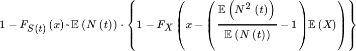
Early references to higher‐order asymptotic approximations for heavy tails are Embrechts et al. [326, 337] and Taylor [731], see also Willmot [785]. As illustrated in Section 6.6, the first‐order asymptotic approximation (6.2.18) is rather inaccurate for not extremely large values of x, but it also turns out to be remarkably robust with respect to dependence (e.g., see Asmussen et al. [66], Albrecher et al. [15]), which may be considered both an advantage and a disadvantage. Segers and Robert [651] show that if the claim number distribution is more heavy tailed than the claim size distribution, then in certain situations one can replace the claim size (rather than the claim number) by its mean in the first‐order approximation.

The mathematical principle underlying the Panjer recursion can be traced back all the way to Euler [341] and has also reappeared early in computer science (see Exercise 7.4 in Knuth [495]). For its first application in actuarial science, see Williams [781] and Panjer [600, 601]. For generalizations, see, for example, Willmot et al. [787] and Dhaene et al. [287]. For a detailed survey of recursive methods we refer to Klugman et al. [491] and Sundt and Vernic [722], who also discuss recursive methods in higher dimensions. For a recent contribution see Rudolph [658]. Numerical inversion of characteristic functions have a long history in risk theory (e.g., see Bohman [144] and Seal [693]). Early references for the FFT method in aggregate claim approximations are Bertram [131] and Bühlmann [167].

Chains of XL treaties are covered, for example, in Albrecher and Teugels [29].

We would like to emphasize that the calculation of the VaR values in Tables 6.1 and 6.2 here for simplicity was done for the fitted distribution, as if this fitted distribution is the true one. However, if the parameter uncertainty due to the estimation procedure were taken into account, the resulting VaR values would be different. In fact, in most applications this effect is overlooked or ignored. However, one should be aware that this can lead to systematic underestimation of VaR values and other risk measures. See Pitera and Schmidt [621] for a recent analysis and illustration.

For an embedding of risk models with causal dependence between claim sizes and their inter‐occurrence times into a semi‐Markovian framework, see, for example, Albrecher and Boxma [16]. Albrecher and Teugels [28] propose a dependence structure between claim sizes and inter‐occurrence times that still preserves a certain random walk structure and is hence quite tractable. For an illustration on how conditional independence of risks given a common random parameter can lead to Archimedean dependence structures, see Albrecher et al. [18] and Constantinescu et al. [224]. A possible source of dependence in data is also a hidden common trend (like neglected inflation etc.); for a study of the consequences of failing to detect such trends on quantiles of compound Poisson sums with heavy‐tailed summands, see Grandits et al. [407].

Classical references for copula techniques are Joe [467] and Nelsen [589] and for an early insurance application Frees and Valdez [359]. A rich source for the application of copulas in risk management is McNeil et al. [568]. For a general approach to a hierarchical pair‐copula construction, see, for example, Aas et al. [1]. Since particularly in the reinsurance context often the number of available data points is not sufficient to identify an appropriate copula for given marginal distributions, it is natural to look for best‐case and (particularly) worst‐case bounds for quantiles (the VaR) of the sum of dependent risks, see, for example, Embrechts et al. [334–336] and Bernard et al. [124]. For the practical computation of such bounds, Puccetti and Rüschendorf [635] developed the so‐called rearrangement algorithm. Since these bounds will in general be quite wide, there has been quite a lot of research activity in how to narrow these bounds under additional information such as higher moments of the sum, see, for example, Bernard et al. [121, 126, 128] and Puccetti et al. [636]. Bignozzi et al. [134] investigated the asymptotic behavior of the VaR of the sum of risks relative to the sum of the individual VaRs under dependence uncertainty. For an assessment of the robustness of VaR and ES with respect to dependence uncertainty, see Embrechts et al. [338] and also Cai et al. [177] for more general risk measures. The tradeoff between robustness and consistent risk ranking is investigated in Pesenti et al. [613]. Filipović [349] compares a bottom‐up approach for risk aggregation to the multi‐level aggregation structure inherent in some standard models of regulators.

In some situations with dependence one can avoid formulating and calibrating the dependence model directly. As an example, for storm risk modelling in Austria, Prettenthaler et al. [633] used a building‐value‐weighted wind index for each region for which aggregate claim data were available to relate the losses to wind speed during the storm. Using the suitably normalized claim data, and implementing a region‐specific correction factor (taking into account the topography and type of buildings of each region) as well as a storm‐specific correction factor (considering the different duration, torsion etc. of each storm), such a relationship could be established. One could then use previous wind field data (that go back in time much longer than the storms for which claim data are available) to create additional loss scenarios and then use resampling techniques to determine global and local loss quantiles. For flood loss modelling, one can alternatively sometimes use concrete risk zonings (produced by experts on‐site) that assign return periods of floods to each local region throughout a country (such zonings exist with remarkable resolution). Together with a map of buildings one can assign losses to each return period, and the dependence modelling then reduces to model the joint occurrence of return periods across these regions, see Prettenthaler et al. [631] for a case study in Austria.

Finally, note that for most of the models exhibiting some sort of dependence between the individual risks, the only way to approximate the aggregate claim distribution or, more particularly, its quantiles, is stochastic simulation, which is discussed in Chapter 9.