
4
Statistics for Claim Sizes
If there is any suspicion of heavy‐tailed distributions, then it is advisable that the actuary should make a number of different data plots. Modelling of large claims is quite an uncertain undertaking, and hence the more graphs considered the better in order to make a balanced conclusion.
As a baseline distribution one might depart from the exponential distribution and inspect for HTE tails. If the right tail of the distribution is obviously heavier than any exponential distribution, then Weibull, log‐normal or Pareto quantile plots offer potential improvements. Such a first step can be performed using different kinds of quantile plots (exponential, log‐normal, Weibull or Pareto) and their derivative plots.
After this large claims modelling using extreme value methodology comes into play. Here the maximum likelihood methodology applied to the peaks over threshold (POT) approach plays the central role. We also emphasize methods based on quantile plotting in order to allow for graphical validation of the models and results. We first discuss the classical case of independence and identically distributed data, followed by regression settings, censored and multivariate data. In reinsurance, the development of large claims can take several years. When evaluating a portfolio, not all the claims are fully developed and the indexed payments at the last available development year are an underestimation of the real final indexed payment. When historical incurred information per claim is available, this should assist in the estimation of the tails of the payment distribution.
It remains desirable to construct a distribution with an appropriate tail fit but which at the same time has enough parameters to fit also in the medium range. An early reference here is Albrecht [32], who pointed out that claim size data are often well described by a Pareto distribution for large claims, while the log‐normal distribution provides a good fit for medium‐sized claims. For a general review on the construction of mixture models with tail components, see Scarott and MacDonald [667]. Here we discuss the method of splicing different distributions in more detail, and in particular we propose combining a mixed Erlang distribution with a tail fit.
All of this material will be illustrated using the data sets introduced in Chapter 1. While the automobile liability data and the Dutch fire insurance data will be used throughout, we end the chapter by analysing the Austrian storm risk, European flood risk data, the Groningen earthquake data, and the Danish fire insurance case in order to illustrate statistical methods for tail estimation.
For a more general survey and statistical methods of extreme value theory see Embrechts et al. [329], Reiss et al. [645], Coles [221], and Beirlant et al. [100]. These references also contain more technical details that are omitted here.
4.1 Heavy or Light Tails: QQ‐ and Derivative Plots
As discussed in Section 3.4 the mean excess function offers a first tool to discriminate between HTE and LTE tails. In practice, based on a sample X1, X2, …, Xn, the mean excess function ![]() can be naively estimated when replacing the expectation by its empirical counterpart:
can be naively estimated when replacing the expectation by its empirical counterpart:

where for any set A, 1A(Xi) equals 1 if Xi ∈ A, and 0 otherwise. The value t is often taken equal to one of the data points, say the (k + 1)‐largest observation Xn−k, n for some k = 1, 2, …, n − 1. We then obtain

The mean excess values ek, n can be plotted as a function of the threshold xn−k, n or as a function of the inverse rank k.
There is an interesting link between the values ek, n and exponential QQ‐plots. For an exponential distribution the quantile values  stand in linear relationship to the corresponding quantiles of the standard exponential distribution
 ![]() :
:
Hence, when estimating  by the empirical quantiles Xj, n, we have that the exponential QQ‐plot, defined by

should exhibit a linear pattern which passes through the origin for the exponential model to be a plausible model. An estimator of the slope can then also be used as an estimator of 1/λ.
Now ek, n can be viewed as an estimate of the slope 1/λk of the exponential QQ‐plot to the right of an anchor point ![]() , and hence (xn−k, n, ek, n) or (k, ek, n) for k = 1, …, n, can be interpreted as a derivative plot of the exponential QQ‐plot. When fitting a regression line which passes through the anchor point using least squares regression minimizing
, and hence (xn−k, n, ek, n) or (k, ek, n) for k = 1, …, n, can be interpreted as a derivative plot of the exponential QQ‐plot. When fitting a regression line which passes through the anchor point using least squares regression minimizing

with respect to 1/λk, one indeed obtains

so that ![]() using the approximation
using the approximation ![]() , which is sharp even for small k.
, which is sharp even for small k.
Also, when the data come from a distribution with a tail heavier than exponential, the exponential QQ‐plot will ultimately be convex and ultimately upcross the fitted regression line for every k, so that the slopes ek, n will increase always with increasing Xn−k, n (or decreasing k), while for a tail lighter than exponential, the QQ‐plot will ultimately be concave, ultimately appearing under the fitted regression line for every k, and the slopes will decrease with increasing Xn−k, n (or decreasing k).
When modelling reinsurance claim data we expect convex exponential QQ‐plots linked with increasing mean excess plots (xn−k, n, ek, n). A popular second step is to inspect log‐normal or Pareto QQ‐plots. Note that the mean excess plots of a Pareto‐type distribution ultimately will be linear increasing with slope 1/(α − 1), as follows from (3.4.12). Again, log‐normal, respectively Pareto, tail fits appear appropriate when the right upper end of the corresponding QQ‐plot is linear from some point on. It is advisable to accompany the QQ‐plot with the corresponding derivative plots.
- Since log X is exponentially distributed with λ = α when X is strict Pareto(α) distributed, the Pareto QQ‐plot is defined aswith derivative plot
 whereHk, n is the estimator of 1/α introduced by Hill [442]. Indeed, if the data come from a Pareto distribution, then the Pareto QQ‐plot is linear and the derivative plot is horizontal at the level 1/α.
- The normal QQ‐plot based on the logarithms of the data provides the log‐normal QQ‐plotwhere Φ−1 denotes the standard normal quantile function. The derivative plot is then given by
 with
with since, with φ denoting the standard normal density,

- The quantile function of the Weibull distribution is given byso that for this model

 . Again taking
  (i = 1, …, n) and estimating Q(i/(n + 1)) by Xi, n leads to the definition of the Weibull QQ‐plotThe derivative plot is then given by
 with
with


Insurance claim data often exhibit different statistical behavior over various subsets of the outcome set which can be observed in mean excess plots, starting with components in the center of the data followed by a Pareto tail. Sometimes such Pareto tails then turn out to be upper‐truncated, as defined in Section 3.3.1.1.


Figure 4.1 Dutch fire insurance data: exponential QQ‐plot and mean excess plot (xn−k, n, ek, n) (top); Pareto QQ‐plot and Hill plot  (second line); log‐normal QQ‐plot and derivative plot
  (third line); Weibull QQ‐plot and derivative plot
  (bottom). For each QQ‐plot the regression line through Xn−99, n, …, Xn, n is plotted.


Figure 4.2 MTPL data for Company A, ultimate data values at evaluation: exponential QQ‐plot and mean excess plot (xn−k, n, ek, n) (top); Pareto QQ‐plot and Hill plot  (second line); log‐normal QQ‐plot and derivative plot
  (third line); Weibull QQ‐plot and derivative plot
  (bottom).


Figure 4.3 MTPL data for Company B, ultimate data values at evaluation: exponential QQ‐plot and mean excess plot (xn−k, n, ek, n) (top); Pareto QQ‐plot and Hill plot  (second line); log‐normal QQ‐plot and derivative plot
  (third line); Weibull QQ‐plot and derivative plot
  (bottom).
4.2 Large Claims Modelling through Extreme Value Analysis
4.2.1 EVA for Pareto‐type Tails
In order to model large claims, Pareto tail modelling is probably the most common approach. Here we use the subset of models with tails heavier than exponential for which the EVI γ is positive, as discussed in Section 3.3.2.2, which in fact equals the set of Pareto‐type models that can be defined through tail functions 1 − F, quantile functions Q, or tail quantile functions U(x) = Q(1 − 1/x). Indeed
where γ = 1/α > 0 and ℓU is a slowly varying function. Also (3.2.7) is equivalent to

for every u > 0. In this section we discuss the estimation of γ = 1/α, large quantiles Q(1 − p) = U(1/p), and small tail probabilities ![]() . We assume in this and the next subsection that the data are independent and identically distributed (i.i.d.). Moreover mathematical approximations of variances (AVar), bias (ABias), mean squared error (AMSE), and distributions of estimators using k largest observations of the n data will hold when
. We assume in this and the next subsection that the data are independent and identically distributed (i.i.d.). Moreover mathematical approximations of variances (AVar), bias (ABias), mean squared error (AMSE), and distributions of estimators using k largest observations of the n data will hold when ![]() and k/n → 0.
and k/n → 0.
4.2.1.1 Estimating a Positive EVI
The most popular estimator for γ is given by the Hill estimator Hk, n defined in (4.1.2), see [442]. In the preceeding section this estimator was retrieved through regression on the Pareto QQ‐plot. Here, we also show how the maximum likelihood method based on the so‐called POT approach leads to the same estimation method in the Pareto‐type case.
- In Section 4.1 the Hill estimator was motivated as an estimator of the slope of a linear Pareto QQ‐plot to the right of an anchor point
 . In fact, this interpretation can be carried over to the general case of Pareto‐type distributions since then ultimately for
  the Pareto QQ‐plot is still linear with slope γ for a small enough k or, equivalently, for a large enough Xn−k, n. Indeed, under (4.2.3),It can now be shown that for every slowly varying function ℓ
 as
as
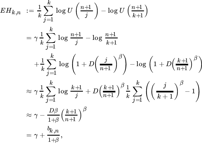
 . Hence, whereas Pareto QQ‐plots are hardly ever completely linear, they are ultimately linear at some set of largest values. The speed at which the linearity sets in depends on the underlying slowly varying function. Like many publications, following Hall [419], we assume here that for some C, β > 0, and D a real constant. This can, however, be generalized toas
 with b essentially a power function or, more correctly, a regularly varying function with index − β, and
  . Under (4.2.5) from which Hk, n follows taking x = (n + 1)/j (j = 1, …, k), estimating U((n + 1)/j) by Xn−j+1, n (j = 1, …, k + 1), and taking the average of both sides of (4.2.6) over j = 1, …, k after deleting the last term on the right‐hand side. Omitting this final term (or, equivalently, assuming a strict Pareto distribution with constant slowly varying function) causes a bias which will be more important with smaller β. Adverse situations for the Hill estimator are logarithmic slowly varying functions ℓU, as in case of the log‐gamma distribution. Such cases exhibit β = 0.
 - Alternatively, the Hill estimator is also a maximum likelihood estimator based on (4.2.4). Indeed, extreme value methodology proposes fitting the limiting Pareto distribution with distribution function 1 − x−1/γ to the POT values Y = X/t over a high threshold t conditionally on X > t. Note that the use of the mathematical limit in (4.2.4) to fit the exceedance data introduces an approximation error that leads to estimation bias. Let Nt denote the number of exceedances over t. Then the log‐likelihood equalswith
 leading to the maximum likelihood estimator
 Choosing an upper order statistic Xn−k, n for the threshold t (so that Nt = k) we obtain Hk, n.
- From Section 4.1 it also follows that the Hill statistic can be interpreted as an estimator of the mean excess function of the log‐transformed data, that is,
 , with the threshold value t substituted by Xn−k, n. As in (3.4.10) we here findEstimating F(u) using the empirical distribution function
 (4.2.7)with value
 over the interval [Xn−j, n, Xn−j+1, n) we are led to the estimator Using summation by parts one observes that this final expression equals the Hill estimator: with(with
 ).
).


To deduce approximate expressions for the variance and bias of the Hill estimator it is helpful to consider the preceding interpretation in terms of the scaled log‐spacings Zj. Thanks to the Rényi representation j(En−j+1, n − En−j, n) = d Ej (j = 1, …, n) concerning order statistics E1, n ≤ E2, n ≤ … ≤ En, n from a random sample E1, E2, …, En of n independent standard exponential random variables, we have in case of a strict Pareto distribution (i.e., with ℓU constant), that
This representation is based on the memoryless property of the exponential distribution and the fact that nE1, n is standard exponentially distributed. From (4.2.9) and (4.2.10) we expect that, as ![]() ,
,

Concerning the bias due to the approximation error, we confine ourselves to the model (4.2.5). Then the theoretical analogue of the Hill estimator is given by
with ![]() . Hence, the approximate mean squared error is given by
. Hence, the approximate mean squared error is given by

while in order to construct confidence bounds we have that, as ![]() with k/n → 0,
with k/n → 0,


Figure 4.4 Pareto QQ‐plot and Hill plot (k, Hk, n): Dutch fire insurance data with 95% confidence intervals for each k (top); MTPL data for Company A, ultimate values (middle); MTPL data for Company B, ultimate values (bottom).
4.2.1.2 Estimating Large Quantiles and Small Tail Probabilities
One of the most important applications of EVA is the estimation of extreme quantiles qp = Q(1 − p) with p small, also termed Value‐at‐Risk (VaR) in risk applications. Alternatively, the return period for a high claim amount x given by ![]() is another measure describing extreme risks.
is another measure describing extreme risks.
The estimation of a high quantile under Pareto‐type modelling can be performed by extrapolating along a fitted regression line on the Pareto QQ‐plot through the point ![]() with slope Hk, n. Following (4.2.6) with x = 1/p, estimating U((n + 1)/(k + 1)) by Xn−k, n and γ by Hk, n, and omitting the second term on the right‐hand side, that is, using
with slope Hk, n. Following (4.2.6) with x = 1/p, estimating U((n + 1)/(k + 1)) by Xn−k, n and γ by Hk, n, and omitting the second term on the right‐hand side, that is, using

we arrive at the estimator

which was first proposed by Weissman [777]. The estimator ![]() can also be retrieved from (4.2.3), leading to the approximation U(vx)/U(x) ≈ vγ for large values of x. Setting vx = 1/p, x = (n + 1)/(k + 1) so that v = (k + 1)/((n + 1)p), and estimating U((n + 1)/(k + 1)) by Xn−k, n and γ by Hk, n, we obtain
can also be retrieved from (4.2.3), leading to the approximation U(vx)/U(x) ≈ vγ for large values of x. Setting vx = 1/p, x = (n + 1)/(k + 1) so that v = (k + 1)/((n + 1)p), and estimating U((n + 1)/(k + 1)) by Xn−k, n and γ by Hk, n, we obtain ![]() again.
again.
Estimation of return periods can be obtained using the inverse relationship on the Pareto QQ‐plot:

The expression for ![]() can also be deduced from (4.2.4), leading to the approximation
can also be deduced from (4.2.4), leading to the approximation ![]() for large values of t. Setting tu = x, t = Xn−k, n so that u = x/Xn−k, n, and estimating
for large values of t. Setting tu = x, t = Xn−k, n so that u = x/Xn−k, n, and estimating ![]() by (k + 1)/(n + 1) we obtain
by (k + 1)/(n + 1) we obtain ![]() .
.
Approximate confidence bounds for such parameters have been derived based on asymptotic distributions of the estimators. In the case of the tail probability estimator we find with ![]()

when ![]() , k/n → 0, npx/k → τ ∈ [0, 1) and
, k/n → 0, npx/k → τ ∈ [0, 1) and ![]() , while with qp = Q(1 − p),
, while with qp = Q(1 − p),

when ![]() , k/n → 0, np/k → τ ∈ [0, 1) and
, k/n → 0, np/k → τ ∈ [0, 1) and ![]() .
.
4.2.1.3 Bias Reduction
When constructing confidence intervals for risk measures such as px and qp, again the approximation of the underlying conditional distribution by the simple Pareto distribution entails a bias for all the existing estimators, next to the bias induced by estimating γ. One approach to reduce the bias is to construct estimators based on regression models of the values Zj. Indeed, under (4.2.5), using the approximation ![]() and with the mean value theorem on x−β at the points j/(n + 1) and (j + 1)/(n + 1), the theoretical analogue of a Zj random variable can be approximated by
and with the mean value theorem on x−β at the points j/(n + 1) and (j + 1)/(n + 1), the theoretical analogue of a Zj random variable can be approximated by


An alternative representation, using 1 + u ≈ eu for small values of u, is then

The more accurate approximation

where Ej denotes a sequence of independent standard exponentially distributed random variables, was derived in an asymptotic sense in Beirlant et al. [97]. For each k, model (4.2.15) can be considered as a non‐linear regression model in which one can estimate the intercept γ, the slope bk, n, and the power β with the covariates j/(k + 1). One can estimate these parameters jointly, or by using an external estimate for β, or using external estimation for β and ![]() on the regression model
on the regression model

Gomes et al. found that external estimation for B and β should be based on k1 extreme order statistics where k = o(k1) and ![]() . Such an estimator for β was presented, for example, in Fraga Alves et al. [35]. Given an estimator
. Such an estimator for β was presented, for example, in Fraga Alves et al. [35]. Given an estimator ![]() for β, an estimator for B was given in Gomes and Martins [399]:
for β, an estimator for B was given in Gomes and Martins [399]:

When the three parameters are jointly estimated for each k, the asymptotic variance turns out to be γ2((1 + β)/β)4, which is to be compared with the asymptotic variance γ2 for the Hill estimator. Performing linear regression on  importing an external estimator for β, the asymptotic variance drops down to γ2((1 + β)/β)2. The original variance γ2 is retained when using the external estimators for B and β in (4.2.16).
Bias reduction of the extreme quantile estimator ![]() should not be based solely on replacing Hk, n by a bias‐reduced estimator for γ. Here we use the fact that Xn−k, n = dU(1/Uk+1, n), where Uk+1, n denotes the (k + 1)th smallest order statistic from a uniform (0,1) sample of size n. Then we obtain from (4.2.3) and (4.2.5) with x = 1/p, approximating Uk+1, n by its expected value (k + 1)/(n + 1), and using 1 + u ≈ eu for u small, that
should not be based solely on replacing Hk, n by a bias‐reduced estimator for γ. Here we use the fact that Xn−k, n = dU(1/Uk+1, n), where Uk+1, n denotes the (k + 1)th smallest order statistic from a uniform (0,1) sample of size n. Then we obtain from (4.2.3) and (4.2.5) with x = 1/p, approximating Uk+1, n by its expected value (k + 1)/(n + 1), and using 1 + u ≈ eu for u small, that

so that a bias‐reduced version of ![]() is given by
is given by

where ![]() , and
, and ![]() are bias‐reduced estimators based on the regression model (4.2.15).
are bias‐reduced estimators based on the regression model (4.2.15).
Bias‐reduced estimators can also be obtained by improving on the approximation (4.2.4) of the POT distribution ![]() by the simple Pareto distribution, using an extension of the Pareto distribution as introduced in Beirlant et al. [102]. Indeed, when ℓU satisfies (4.2.5), then
by the simple Pareto distribution, using an extension of the Pareto distribution as introduced in Beirlant et al. [102]. Indeed, when ℓU satisfies (4.2.5), then
The distribution of the POT’s X/t (X > t) can then be approximated using the expansion (1 + u)b ≈ 1 + bu for u small:

This leads to the extended Pareto distribution (EPD) with distribution function
(![]() ) with δ = δt = DCβ/γt−β/γ and τ = −β/γ. Note that for an EPD random variable Y with τ = −1 and
) with δ = δt = DCβ/γt−β/γ and τ = −β/γ. Note that for an EPD random variable Y with τ = −1 and ![]() , it follows that Y − 1 is GPD distributed with parameters γ and σ.
, it follows that Y − 1 is GPD distributed with parameters γ and σ.
Using the density of the EPD gγ, δ, τ(y) = γ−1y−1/γ−1{1 + δ(1 − yτ)}−1/γ−1[1 + δ{1 − (1 + τ)yτ}], maximum likelihood estimators are then derived through maximization of

with respect to γ, δ using an external estimator of τ through estimates of β and γ, where the values ![]() denote the POT values over the threshold t.
denote the POT values over the threshold t.
Bias‐reduced estimation of return periods is then obtained using Xn−k, n again as a threshold t:

4.2.1.4 Estimating the Scale Parameter
Finally, note that the scale parameter C in (4.2.5), or A = C1/γ in (4.2.17), can be estimated with
which follows, for instance, from (4.2.17) replacing x by Xn−k, n and estimating ![]() by the empirical probability (k + 1)/(n + 1).
by the empirical probability (k + 1)/(n + 1).
The estimator Ĉk,n can also be retrieved using least squares regression on the k top points of the log–log plot

minimizing

Substituting Hk, n for γ and taking the derivative with respect to log C indeed gives

In Beirlant et al. [104] it is shown that Âk,n is asymptotically normally distributed with asymptotic variance ![]() and asymptotic bias
and asymptotic bias ![]() .
.
A bias‐reduced estimator of the scale parameter A is then given by

where ![]() is a bias‐reduced estimator of γ, and
is a bias‐reduced estimator of γ, and ![]() estimators of bk, n and β.
estimators of bk, n and β.


Figure 4.5 Hill estimates and bias‐reduced versions, regression approach as a function of k (left) and log k (right), and EPD approach (middle) as a function of k: Dutch fire insurance data (top); MTPL data for Company A, ultimate values (middle); MTPL data for Company B, ultimate values (bottom).

Figure 4.6 Quantile estimates  and
and  (left) and log‐return periods
  and
and  (right), as a function of k: Dutch fire insurance data (x = 200 million, top); MTPL data for Company A, ultimate values (x = 4 million, middle); MTPL data for Company B, ultimate values (x = 6 million, bottom).

Figure 4.7 Scale estimates Âk,n and  as a function of k: Dutch fire insurance data (top); MTPL data for Company A, ultimate values (middle); MTPL data for Company B, ultimate values (bottom).
4.2.2 General Tail Modelling using EVA
In order to allow tail modelling with log‐normal or Weibull tails, one has to incorporate the case where the EVI γ can be 0, next to positive values. Estimation of γ, extreme quantiles and return periods under the max‐domains of attraction conditions Cγ in (3.2.5) or (3.2.6), with as few restrictions on the value of γ as possible, is the next step in tail modelling. Again we have two possible approaches: using quantile plotting or using a likelihood approach on POT values.
- Here, several existing estimators start from the following condition, which follows from (3.2.5): for all u ≥ 1 as
 (4.2.22)From this it follows with
 , that as
  , k/n → 0
Hence estimating EHk, n by Hk, n, and
 by Xn−k, n, we find that for any estimator
  of γ
of γleads to an estimator for
 .
.Since a regularly varies with index
 , it also follows from (4.2.23) that U((n + 1)/(k + 1))EHk, n = ((n + 1)/(k + 1))γℓ((n + 1)/(k + 1)) for some slowly varying function ℓ. Hence the approach using linear regression and extrapolation on linear tail patterns on a QQ‐plot can be generalized to the case of a real‐valued EVI using the generalized QQ‐plot
which ultimately for smaller values of k will be linear with slope γ, whatever the sign or values of γ. Hence if a generalized QQ‐plot is ultimately horizontal, then tail modelling using a distribution in the Gumbel domain of attraction is appropriate. An ultimately decreasing generalized QQ‐plot indicates a negative EVI, which can occur, for instance, for truncated heavy‐tailed distributions.
A generalized Hill estimator of γ estimating the slopes at the last k points on the generalized QQ‐plot is then given by

where UHj, n = Xn−j, nHj, n.
Another generalization of the Hill estimator to real‐valued EVI was given in Dekkers et al. [268], termed the moment estimator:

where
- Condition (3.2.6) for a distribution to belong to a domain of attraction of an extreme value distribution means that the generalized Pareto law is the limit distribution of the distribution of POT values X − t given X > t when t → x+: setting h(t) = σt Hence, we are led to modelling the tail function
 of POT values Y = X − t with X > t using the GPD with survival function
  . Denoting the number of exceedances over t again by Nt, the log‐likelihood is given byUsing a reparametrization (γ, σ) → (γ, τ) with τ = γ/σ, leads to the likelihood equations
 Replacing t by an intermediate order statistic Xn−k, n again gives
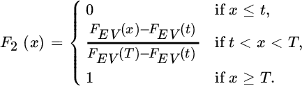
 In order to assess the goodness‐of‐fit of the GPD when modelling the POT values Y = X − t for a given threshold t, one can use the transformation
 so that R is standard exponentially distributed if the POT values do follow a GPD, and the fit can be validated inspecting the overall linearity of the exponential QQ‐plot
 where
where
 (i = 1, …, Nt) denote the ordered values of


For all these estimators ![]() is asymptotically normal under some regularity conditions on the underlying distributions when
is asymptotically normal under some regularity conditions on the underlying distributions when ![]() and k/n → 0, with mean 0 if k is not too large (or, equivalently, if the threshold t = xn−k, n is not too small), and asymptotic variances (or covariance matrix for
and k/n → 0, with mean 0 if k is not too large (or, equivalently, if the threshold t = xn−k, n is not too small), and asymptotic variances (or covariance matrix for ![]() ) given by
) given by

Estimators for small tail probabilities or return periods can easily be constructed from the POT approach. In fact, the approximation of P(X − t > y|X > t) by (1 + (γ/σ)y)−1/γ for y > 0, setting t + y = x, leads to

Inversion leads to an extreme quantile estimator

The estimators for high quantiles based on the approach used in the construction of the moment estimator ![]() are defined by
are defined by

with â defined in (4.2.24). Note that ![]() can be seen as an alternative estimator for σ when comparing the expressions of
can be seen as an alternative estimator for σ when comparing the expressions of ![]() and
and ![]() . This then in turn leads to a moment tail probability estimator
. This then in turn leads to a moment tail probability estimator

The asymptotic distributions of these tail estimators have been derived in the literature. For instance, for ![]() we have under some regularity conditions that with an = (k + 1)/(p(n + 1)) as npn → c ≥ 0,
we have under some regularity conditions that with an = (k + 1)/(p(n + 1)) as npn → c ≥ 0, ![]() one has
one has
- for γ > 0

- for γ < 0

For further details see de Haan and Ferreira [258].


Figure 4.8 Generalized QQ‐plot (middle) and estimators of EVI  ,
,  ,
,  as a function of k (left) and log k (right): Dutch fire insurance data (first and second line); MTPL data for Company A, ultimate values (third and fourth line); MTPL data for Company B, ultimate values (bottom two lines).

Figure 4.9 Large quantile estimators  ,
,  ,
,  (left) and log‐return period estimators
  ,
,  ,
,  (right) as a function of k: Dutch fire insurance data (x = 200 million, top); MTPL data for Company A, ultimate values (x = 4 million, middle); MTPL data for Company B, ultimate values (x = 6 million, bottom).
4.2.3 EVA under Upper‐truncation
Practical problems can arise when using the strict Pareto distribution and its generalization to the Pareto‐type model because some probability mass can still be assigned to loss amounts that are unreasonably large or even impossible. With respect to tail fitting of an insurance claim data, upper‐truncation is of interest and can be due to the existence of a maximum possible loss. Such truncation effects are sometimes visible in data, for instance when an overall linear Pareto QQ‐plot shows non‐linear deviations at only a few top data. Let W be an underlying non‐truncated distribution with distribution function FW, quantile function QW and tail quantile function UW. Upper‐truncation of the distribution of W at some value T was defined in the preceding chapter through the conditioning operation W|W < T. Let FT and UT be the distribution and tail quantile function of this truncated distribution. In practice one does not always know if the data X1, …, Xn come from a truncated or non‐truncated distribution, and hence the behavior of estimators should be evaluated under both cases, and a statistical test for upper‐truncation is useful. This section is taken from Beirlant et al. [95].
Upper‐truncation of the distribution of W at some truncation point T yields

The corresponding quantile function QT is then given by
while the tail function UT satisfies

or

with ![]() the odds of the truncated probability mass under the untruncated distribution W. Note also that for a fixed T, upper‐truncation models are known to exhibit an EVI γ = −1. This follows from verifying (3.2.5) for UT as given in (4.2.27). For instance when UW(x) = xγ, we find
the odds of the truncated probability mass under the untruncated distribution W. Note also that for a fixed T, upper‐truncation models are known to exhibit an EVI γ = −1. This follows from verifying (3.2.5) for UT as given in (4.2.27). For instance when UW(x) = xγ, we find  as
as ![]() . This final expression satisfies (3.2.5) with γ = −1.
. This final expression satisfies (3.2.5) with γ = −1.
4.2.3.1 EVA for Upper‐truncated Pareto‐type Distributions
We restrict attention to tail estimation for upper‐truncated Pareto‐type distributions:
where ℓF is a slowly varying function at infinity or, with W/t denoting the peaks over a threshold t when W > t,
Upper‐truncation of a Pareto‐type distribution at a high value T then necessarily requires ![]() and
and

One can now consider two cases as ![]() :
:
- Rough upper‐truncation with the threshold t when T/t → β > 1 and This corresponds to situations where the deviation from the Pareto behavior due to upper‐truncation at a high value will be visible in the data from the threshold t onwards, and an adaptation of the above Pareto tail extrapolation methods appears appropriate.
- Light (or no) upper‐truncation with the threshold t: when
 (4.2.29)and hardly any truncation is visible in the data from the threshold t onwards, and the Pareto‐type model without truncation and the corresponding extreme value methods for Pareto‐type tails appear appropriate when restricted to excesses over t.

Under rough upper‐truncation we have

with density

Estimating T by Xn, n and taking t = Xn−k, n so that ![]() , we obtain the following log‐likelihood:
, we obtain the following log‐likelihood:

Now

which leads to the defining equation for the likelihood estimator ![]() :
:

This estimator was first proposed in Aban et al. [6]. Beirlant et al. [95] showed that with κ = β1/γ − 1

From (4.2.27) it is clear that the estimation of DT is an intermediate step in important estimation problems following the estimation of γ, namely of extreme quantiles and of the endpoint T. When UW satisfies (4.2.3) it follows from (4.2.27) that as ![]() and T/t → β
and T/t → β

so that

Motivated by (4.2.31) and estimating QT(1 − (k + 1)/(n + 1))/QT(1 − 1/(n + 1)) by Rk, n, one arrives at

as an estimator for DT. In practice one makes use of the admissible estimator

to make it useful for truncated and non‐truncated Pareto‐type distributions.
For DT > 0, in order to construct estimators of T and extreme quantiles qp = QT(1 − p), as in (4.2.31) we find that

Then taking logarithms on both sides of (4.2.33) and estimating QT(1 − (k + 1)/(n + 1)) by Xn−k, n we find an estimator ![]() of qp:
of qp:

which equals the Weissman estimator ![]() when
when ![]() . An estimator
. An estimator ![]() of T follows from letting p → 0 in the above expressions for
of T follows from letting p → 0 in the above expressions for ![]() :
:

Here we take the maximum of log Xn,n and the value following from (4.2.34) with p → 0 in order for this endpoint estimator to be admissible. It has been shown that ![]() is superefficient under rough upper‐truncation, which means that the asymptotic variance is o(1/k) and the asymptotic bias is also smaller than, for instance, that of the moment quantile estimator
is superefficient under rough upper‐truncation, which means that the asymptotic variance is o(1/k) and the asymptotic bias is also smaller than, for instance, that of the moment quantile estimator ![]() .
.
However, ![]() is not a consistent estimator for qp under light upper‐truncation and when npn → 0. In that case one should use
is not a consistent estimator for qp under light upper‐truncation and when npn → 0. In that case one should use

The estimation of tail probabilities px = P(X > x) can be based directly on (4.2.28) using Rk, n as an estimator for 1/β:

Of course, in order to decide between (4.2.34) and (4.2.36) one should use a statistical test for deciding between rough and light upper‐truncation.
4.2.3.2 Testing for Upper‐truncated Pareto‐type Tails
Aban et al. [6] proposed a test for ![]() versus
versus ![]() under the strict Pareto model, rejecting H0 at level q ∈ (0, 1) when
under the strict Pareto model, rejecting H0 at level q ∈ (0, 1) when

for some 1 < k < n with A the scale parameter in the Pareto model. In (4.2.38), γ is estimated by Hk, n, the maximum likelihood estimator under H0, while A is estimated using Âk,n from (4.2.19). Note that the rejection rule (4.2.38) can be rewritten as

and the P‐value is given by  .
.
Considering the testing problem
under the upper‐truncated Pareto‐type model, Beirlant et al. [95] propose to reject ![]() when an appropriate estimator of (n + 1)DT/(k + 1) is significantly different from 0. Here we construct such an estimator generalizing
when an appropriate estimator of (n + 1)DT/(k + 1) is significantly different from 0. Here we construct such an estimator generalizing ![]() with an average of ratios (Xn−k, n/Xn−j+1, n)1/γ, j = 1, …, k, which then possesses an asymptotic normal distribution under the null hypothesis. Observe that with (4.2.30) under
with an average of ratios (Xn−k, n/Xn−j+1, n)1/γ, j = 1, …, k, which then possesses an asymptotic normal distribution under the null hypothesis. Observe that with (4.2.30) under ![]() as
as ![]()

Estimating Ēk,n by

leads now to

as an estimator of (n + 1)DT/(k + 1), with ![]() an appropriate estimator of γ. Under
an appropriate estimator of γ. Under ![]() , the Hill estimator Hk, n is an appropriate estimator of γ. Moreover, it can be shown that under some regularity assumptions on the underlying Pareto‐type distribution, we have under
, the Hill estimator Hk, n is an appropriate estimator of γ. Moreover, it can be shown that under some regularity assumptions on the underlying Pareto‐type distribution, we have under ![]() for
for ![]() and k/n → 0, that
and k/n → 0, that ![]() is asymptotically normal with mean 0 and variance 1/12. It is then also shown under rough upper‐truncation as
is asymptotically normal with mean 0 and variance 1/12. It is then also shown under rough upper‐truncation as ![]() , k/n → 0 that Lk, n(Hk, n) tends to a negative constant so that an asymptotic test based on Lk, n(Hk, n) rejects
, k/n → 0 that Lk, n(Hk, n) tends to a negative constant so that an asymptotic test based on Lk, n(Hk, n) rejects ![]() on level q when
on level q when
with ![]() . The P‐value is then given by
. The P‐value is then given by ![]() .
.

Figure 4.10 MTPL data for Company A, ultimate estimates:  and Hk, n as a function of k (top left), P‐value of TB, k as a function of k (top right),
  and
and  as a function of k (middle left), estimates of endpoint
  (middle right),
  as a function of k (bottom left), truncated Pareto fit to Pareto QQ‐plot based on top k = 250 observations (bottom right).
4.3 Global Fits: Splicing, Upper‐truncation and Interval Censoring
Given an appropriate tail fit, the ultimate goal consists of fitting a distribution with a global satisfactory fit. Rather than trying to splice specific parametric models such as log‐normal or Weibull models for the modal part of the distribution, one can rely on fitting a mixed Erlang (ME) distribution, as discussed in Verbelen et al. [758]. We also consider this set‐up in the presence of truncation and censoring.
4.3.1 Tail‐mixed Erlang Splicing
The Erlang distribution has a gamma density

where r is a positive integer shape parameter. Following Lee and Lin [534] we consider mixtures of M Erlang distributions with common scale parameter 1/λ having density

and tail function

where the positive integers r = (r1, …, rM) with r1 < r2 < … < rM are the shape parameters of the Erlang distributions, and α = (α1, …, αM) with αj > 0 and ![]() are the weights in the mixture. Tijms [745] showed that the class of mixtures of Erlang distributions with a common scale 1/λ is dense in the space of positive continuous distributions on
are the weights in the mixture. Tijms [745] showed that the class of mixtures of Erlang distributions with a common scale 1/λ is dense in the space of positive continuous distributions on ![]() . Moreover this class is also closed under mixtures, convolution and compounding. Hence aggregate risks calculations are simple, and XL premiums and risk measures based on quantiles can also be evaluated in a rather straightforward way.For instance, a composite ME generalized Pareto distribution can be built using (3.5.14), that is, a two‐component spliced distribution with density
. Moreover this class is also closed under mixtures, convolution and compounding. Hence aggregate risks calculations are simple, and XL premiums and risk measures based on quantiles can also be evaluated in a rather straightforward way.For instance, a composite ME generalized Pareto distribution can be built using (3.5.14), that is, a two‐component spliced distribution with density

If a continuity requirement at t were imposed, this would lead to

The survival function of this spliced distribution is given by

Alternatively, one can take ![]() , where k* is an appropriate number of top order statistics corresponding to an extreme value threshold
, where k* is an appropriate number of top order statistics corresponding to an extreme value threshold ![]() .
.
Fitting ME distributions through direct likelihood maximization is difficult. A first algorithm was proposed by Tijms [745], but it turns out to be slow and can lead to overfitting. Lee and Lin [534] use the expectation‐maximization (EM) algorithm proposed by Dempster et al. [271] to fit the ME distribution. Model selection criteria, such as the Akaike information criterion (AIC) and Bayesian information criterion (BIC) information criteria, are then used to avoid overfitting. Verbelen et al. [758] extend this approach to censored and/or truncated data. The need for the EM algorithm follows from the data incompleteness due to mixing and censoring.
The EM algorithm is used to compute the maximum likelihood estimator (MLE) for incomplete data where direct maximization is impossible. It consists of two steps that are put in an iteration until convergence:
- E‐step: Compute the conditional expectation of the log‐likelihood given the observed data and previous parameter estimates.
- M‐step: Determine a subsequent set of parameter estimates in the parameter range through maximization of the conditional expectation computed in the E‐step.
Rather than proposing a data‐driven estimator of the splicing point t, we use an expert opinion on the splicing point t based on EVA as outlined above. Then, π can be estimated by the fraction of the data not larger than t. Similarly, T is deduced from the EVA. The extreme value index γ is estimated in the algorithm, starting from the value obtained from the EVA at the threshold t. The final estimates for γ always turned out to be close to the EVA estimates. Next, the ME parameters (α, λ) are estimated using the EM algorithm as developed in Verbelen et al. [758]. The number of ME components M is estimated using a backward stepwise search, starting from a certain upper value, whereby the smallest shape is deleted if this decreases an information criterion such as AIC or BIC. Moreover, for each value of M, the shapes r are adjusted based on maximizing the likelihood starting from r = (s, 2 s, …, …, M × s), where s is a chosen spread factor.
Of course tail splicing of an ME can also be performed using a simple Pareto fit, or an EPD fit, whether or not adapted for truncation. For instance, splicing an ME with an upper‐truncated Pareto approximation leads to


Figure 4.11 MTPL data for Company A ultimates: fit of spliced model with a mixed Erlang and a Pareto component with thresholds t indicated on mean excess plot (top left); empirical and model survival function (top right); PP plot of empirical survival function against splicing model RTF (bottom left); idem with  transformation (bottom right).
4.3.2 Tail‐mixed Erlang Splicing under Censoring and Upper‐truncation
In reinsurance data left truncation appears at some point, denoted here by tl, which can be a deductible or a percentage of the retention u from an XL contract. Claims leading to a cumulative payment below tl at a given stage during development are then left truncated. Such a claim constitutes an IBNR claim. As discussed above, an upper‐truncation mechanism at some point T can appear.
We denote the ME density and distribution function by fME and FME, and similarly fEV and FEV for the EVA distribution. We then define, omitting the model parameters from the notation for the moment,


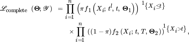
with 0 ≤ tl < t < T where T can be equal to ![]() . The densities f1 and f2 are then valid densities on the intervals [tl, t] and [t, T], respectively. For the first density, this means that it is lower truncated at tl and upper truncated at t, and the second density is lower truncated at t and upper truncated at T. The corresponding distribution functions are
. The densities f1 and f2 are then valid densities on the intervals [tl, t] and [t, T], respectively. For the first density, this means that it is lower truncated at tl and upper truncated at t, and the second density is lower truncated at t and upper truncated at T. The corresponding distribution functions are

We consider the splicing density and distribution function

and

Next to truncation, censoring mechanisms occur in reinsurance1 :
- right censoring occurs for instance when a claim has not been settled at the evaluation date (RBNS claims). See Chapter 1 for the case of motor liability data. The final claim amount xi will be larger than the lower censoring value li
- left censoring occurs when only an upper bound ui to the claim xi is given
- interval censoring means that the final claim value xi is only known to be inside an interval [li, ui] ⊂ [tl, T].
In the splicing context with an EVA component from a threshold t on, we have the following five classes of observations:
- Uncensored observations with tl ≤ li = ui = xi ≤ t < T.
- Uncensored observations with tl < t < li = ui = xi ≤ T.
- Interval censored observations with tl ≤ li < ui ≤ t < T.
- Interval censored observations with tl < t ≤ li < ui ≤ T.
- Interval censored observations with tl ≤ li < t < ui ≤ T.
These classes are shown in Figure 4.12. In the conditioning argument in the E‐step of the algorithm, the fifth case is split into xi ≤ t and xi > t, as indicated in Figure 4.12.

Figure 4.12 The different classes of censored observations.
For the Erlang mixture, the number M and the integer shapes r are fixed when estimating Θ1 = (α, λ). Also, Θ2 denotes the extreme value parameter γ (together with σ when using the GPD tail fit). The idea behind the EM algorithm in this context is to consider the censored sample ![]() in contrast to the complete data
in contrast to the complete data ![]() which is not fully observed. Given a complete version of the data, we can construct a complete likelihood function as
which is not fully observed. Given a complete version of the data, we can construct a complete likelihood function as
where ![]() is the indicator function for the event {Xi ≤ t}. The corresponding complete data log‐likelihood function is
is the indicator function for the event {Xi ≤ t}. The corresponding complete data log‐likelihood function is

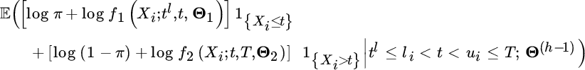
As we do not fully observe the complete version ![]() of the data sample, it is not possible to optimize the complete data log‐likelihood directly. The intuitive idea for obtaining parameter estimates in the case of incomplete data is to compute the expectation of the complete data log‐likelihood and then use this expected log‐likelihood function to estimate the parameters. However, taking the expectation of the complete data log‐likelihood requires the knowledge of the parameter vector, and so the algorithm has to run iteratively. Starting from an initial guess for the parameter vector, the EM algorithm iterates between two steps. In the hth iteration of the E‐step the expected value of the complete data log‐likelihood is computed with respect to the unknown data
of the data sample, it is not possible to optimize the complete data log‐likelihood directly. The intuitive idea for obtaining parameter estimates in the case of incomplete data is to compute the expectation of the complete data log‐likelihood and then use this expected log‐likelihood function to estimate the parameters. However, taking the expectation of the complete data log‐likelihood requires the knowledge of the parameter vector, and so the algorithm has to run iteratively. Starting from an initial guess for the parameter vector, the EM algorithm iterates between two steps. In the hth iteration of the E‐step the expected value of the complete data log‐likelihood is computed with respect to the unknown data ![]() given the observed data
given the observed data ![]() and using the current estimate of the parameter vector Θ(h−1) as true values,
and using the current estimate of the parameter vector Θ(h−1) as true values,
In the M‐step, one maximizes the expected value of the complete data log‐likelihood obtained in the E‐step with respect to the parameter vector:
Both steps are iterated until convergence.
In the E‐step we distinguish the five cases of data points again to determine the contribution of a data point to this expectation:
Note that the event {tl ≤ li = ui ≤ t < T} indicates that we know tl, li = ui, t and T, and that the ordering tl ≤ li = ui ≤ t < T holds. Similar reasonings hold for the other conditional arguments in the expectations. Then, using the law of total probability, the final case can be rewritten as

where {tl ≤ li < Xi ≤ t < ui ≤ T} denotes that tl, li, t, ui and T are known, that the ordering tl ≤ li < t < ui ≤ T holds, and that {Xi ≤ t}. Using (4.3.43) we find that the probability in the first term is then given by

and similarly for the second term. The M‐step with maximization with respect to π, Θ1 and Θ2, and the choice of the initial values, is discussed in detail in Reynkens et al. [647].
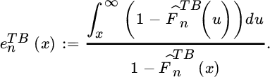
EVA is not available in the literature for interval censored data. The role of the empirical survival and quantile functions in the construction of a tail analysis for complete data (i.e., setting Xn−j+1, n as an estimator of Q(1 − j/(n + 1)), j = 1, …, n) is taken over by the Turnbull [747] estimator ![]() . The Turnbull estimator is an extension to interval censoring of the Kaplan–Meier estimator or product‐limit estimator [482], that is, when
. The Turnbull estimator is an extension to interval censoring of the Kaplan–Meier estimator or product‐limit estimator [482], that is, when ![]() .
.
- The Kaplan–Meier estimator
 of 1 − F is defined as follows: letting 0 = τ0 < τ1 < τ2 < … < τN (with N < n) denote the observed possible censored data, Nj the number of observations Xi ≥ τj, and dj the number of values li equal to τj, thenThis expression is motivated from the fact that

- Turnbull’s algorithm is then constructed as follows: Let 0 = τ0 < τ1 < … < τm denote here the grid of all points li, ui, i = 1, 2, …, n. Define δij as the indicator whether the observation in the interval (li, ui] could be equal to τj, j = 1, …, m. δij equals 1 if (τj−1, τj] ⊂ (li, ui] and 0 otherwise. Initial values are assigned to 1 − F(τj) by distributing the mass 1/n for the ith individual equally to each possible τj ∈ (li, ui]. The algorithm is given as:
- Compute the probability pj that an observation equals τj by pj = F(τj) − F(τj−1), j = 1, …, m.
- Estimate the number of observations at τj by

- Compute the estimated number of data with li ≥ τj by
 .
. - Update the product‐limit estimator using the values of dj and Nj found in the two preceding steps. Stop the iterative process if the new and old estimate of 1 − F for all τj do not differ too much.
In case of interval censored data we can then estimate the mean excess function e (see (3.4.10)) substituting 1 − F by the Turnbull estimator ![]() :
:
As discussed in Section 4.2.1, the mean excess function based on the log‐data leads to an estimator of a positive extreme value index γ. As in (4.2.8), using the Turnbull estimator rather than the classical empirical distribution we obtain an estimator of γ > 0 in the case of incomplete data:

We then compute these statistics at the positions ![]() , k = 1, …, n − 1. Such plots will assist in choosing an appropriate threshold t and estimates of the extreme value index γ to validate the tail component in the splicing.
, k = 1, …, n − 1. Such plots will assist in choosing an appropriate threshold t and estimates of the extreme value index γ to validate the tail component in the splicing.

Figure 4.13 Dutch fire claim data: fit of spliced model mixed Erlang and Pareto with threshold t indicated on the mean excess plot (top left); empirical and model survival function (top right); PP plot of empirical survival function against splicing model RTF (bottom left); idem with  transformation (bottom right).

Figure 4.14 Dutch fire claim data: fit of spliced model with a mixed Erlang and two Pareto components with thresholds t1 and t2 as indicated on the mean excess plot (top left); empirical and model survival function (top right); PP plot of empirical survival function against splicing model RTF (bottom left); idem with  transformation (bottom right).

Figure 4.15 MTPL data for Company A: percentage of closed claims with incurred value being a correct upper bound for final payment as a function of the number of development years (DY) (top); boxplots of Ri, d for every development year d and factor fd used in the interval censoring approach (bottom).

Figure 4.16 MTPL data for Company A: fit of spliced mixed Erlang and Pareto models with interval censoring based on upper bounds Ii, d, i = 1, …, 596, d = 5, …, 16, for non‐closed claims: mean excess plot based on (4.3.44) (top left); Hill plot based on (4.3.45) (top right); empirical and model survival function (middle left); PP plot of empirical survival function against splicing model RTF (middle right); idem with  transformation (bottom).

Figure 4.17 MTPL data for Company A (1995–2009): fit of spliced mixed Erlang and Pareto models with interval censoring based on upper bounds Ĩi,d, i = 1, …, 849, d = 1, …, 15 for non‐closed claims: mean excess plot based on (4.3.44) (top left); Hill plot based on (4.3.45) (top right); empirical and model survival function (middle); PP plot of  survival function, empirical against splicing mode (bottom left); size of confidence intervals using interval censoring with upper bounds Ii, d and Ĩi,d (bottom right).

Figure 4.18 MTPL data for Company B: mean excess plot based on (4.3.44) (top left) and Hill plot based on (4.3.45) (top right) for interval censored data based on accidents from 1990 to 2005; fit of spliced model mixed Erlang and Pareto models: empirical and model survival function (middle left); PP plot of empirical survival function against splicing model RTF (middle right) left); idem with  transformation (bottom).
If the upper bounds are put to ![]() , that is, if one uses the right censoring framework, then, under the random right censoring assumption of independence between the real cumulative payment at closure of the claim and the censoring variable C which is observed in case the claim is right censored, estimators of γ > 0 have been proposed in Beirlant et al. [96, 101], Einmahl et al. [315], and Worms and Worms [796]. Using the likelihood approach, Beirlant et al. [101] proposed the estimator
, that is, if one uses the right censoring framework, then, under the random right censoring assumption of independence between the real cumulative payment at closure of the claim and the censoring variable C which is observed in case the claim is right censored, estimators of γ > 0 have been proposed in Beirlant et al. [96, 101], Einmahl et al. [315], and Worms and Worms [796]. Using the likelihood approach, Beirlant et al. [101] proposed the estimator

with ![]() (i = 1, …, n) and
(i = 1, …, n) and ![]() the proportion of non‐censored data in the top kZ‐data. Einmahl et al. [315] derived asymptotic results, while Beirlant et al. [96] proposed a bias‐reduced version. Worms and Worms [796] derived a tail index estimator which is derived through the estimation of the mean excess function of the log‐data, comparable with the estimator derived in (4.3.45):
the proportion of non‐censored data in the top kZ‐data. Einmahl et al. [315] derived asymptotic results, while Beirlant et al. [96] proposed a bias‐reduced version. Worms and Worms [796] derived a tail index estimator which is derived through the estimation of the mean excess function of the log‐data, comparable with the estimator derived in (4.3.45):

where the Kaplan–Meier estimator can be written as

with Δi, n equal to 1 if the ith smallest observation Zi, n is non‐censored, and 0 otherwise.

Figure 4.19 Hill plots adapted for interval censoring  with upper bounds Ii, d and Ĩi,d, and Hill estimates based on random right censoring
  without upper bounds. The vertical line indicates the splicing threshold t used above.
4.4 Incorporating Covariate Information
In certain instances, the assumption of i.i.d. random variables, underlying the extreme value methods discussed above, may be violated. When analysing claim data from different companies, the tail fits may differ. Also, loss distributions may change over calendar years or along the number of development years. Sometimes considering covariates may remedy the situation. Let the covariate information, whether using continuous or indicator variables, be contained in a covariate vector x = (x1, …, xp). The extension of the POT approach based on (4.2.25) has been popular in literature, starting with the seminal paper by Davison and Smith [253]. However, there are also some methods available that focus on response random variables that exhibit Pareto‐type tails. Here we denote the response variables Zi (rather than Xi as in the preceding sections) with the corresponding exceedances or POTs Y = Z/t or Y = Z − t when Z > t.
4.4.1 Pareto‐type Modelling
When modelling time dependence or incorporating any other covariate information in an independent data setting with Pareto‐type distributed responses Zi, the exceedances are defined through Yi = Zi/t for some appropriate threshold t. Note that in many circumstances the threshold should then also be modelled along x = xi, i = 1, …, n. As before, we assume that as ![]()
where Ai, γi > 0. Regression can be modelled through the scale parameter A and/or the extreme value index γ.
Changes in γ can be modelled in a parametric way using likelihood techniques. Suppose, for instance, that regression modelling of γ > 0 using an exponential link function appears appropriate in a given case study:
The log‐likelihood function is then given by

leading to the likelihood equations

Beirlant and Goegebeur [99] propose to inspect the goodness‐of‐fit of such a regression model under constant scale parameter A on the basis of a Pareto QQ‐plot using
which are indeed approximately Pareto distributed with tail index 1, when the regression model is appropriate.
The case where γ does not depend on i, while A does depend on i, was formalized in Einmahl et al. [316] assuming that there exists a tail function 1 − F and a continuous, positive function A defined on [0, 1] such that

uniformly for all ![]() and all i = 1, …, n with
and all i = 1, …, n with  . A is then called the skedasis function, which characterizes the trend in the extremes through the changes in the scale parameter A. Under (4.4.49), Einmahl et al. [316] showed that the Hill estimator Hk, n is still a consistent estimator for γ. Assuming equidistant covariates xi = i/n, i = 1, …, n, as in (4.2.19),

where  denotes the number of Z values larger than the threshold Zn−k, n with covariate value x in a neighbourhood of xi. The contribution of the observations to
 ![]() is governed by a symmetric density kernel function K on [−1, 1] and Kh(x) = K(x/h)/h, so that K gives more weight to the observations with covariates closer to xi. We hence obtain
is governed by a symmetric density kernel function K on [−1, 1] and Kh(x) = K(x/h)/h, so that K gives more weight to the observations with covariates closer to xi. We hence obtain

Finally, estimators of small tail probabilities and large quantiles follow directly from (4.4.49), (4.2.12) and (4.2.13):

4.4.2 Generalized Pareto Modelling
Let Y1, …, Yn be independent GPD random variables and let xi denote the covariate information vector, that is,

where γ(x), σ(x), μ(x) denote admissible functions of x, whether of parametric nature using three vectors of regression coefficients βj (j = 1, 2, 3) of length p with ![]() ,
, ![]() and
and ![]() , or of non‐parametric nature. Again this model is used as an approximation of the conditional distribution of excesses Y (x) = Z − μ(x) over a high threshold μ(x) given that there is an exceedance. The choice of an appropriate threshold μ(x) is of course even more difficult than in the non‐regression setting since the threshold can depend on the covariates in order to take the relative extremity of the observations into account.
, or of non‐parametric nature. Again this model is used as an approximation of the conditional distribution of excesses Y (x) = Z − μ(x) over a high threshold μ(x) given that there is an exceedance. The choice of an appropriate threshold μ(x) is of course even more difficult than in the non‐regression setting since the threshold can depend on the covariates in order to take the relative extremity of the observations into account.
- When parametric functions
 ,
,  and
and  have been chosen, the estimators of βj (j = 1, 2, 3) can be obtained by maximizing the log‐likelihood functionwhere Nμ denotes the number of excesses over the threshold function μ(x).
- Alternatively, non‐parametric regression techniques are available to estimate the parameter functions γ(x), σ(x). Consider independent random variables Z1, …, Zn and associated covariate information x1, …, xn. Suppose we focus on estimating the tail of the distribution of Z at x*. Fix a high local threshold μ(x*) and compute the exceedances Yi = Zj − μ(x*), provided Zj > μ(x*),
 . Here j is the index of the ith exceedance in the original sample, and
  denotes the number of exceedances over the threshold μx*. Then re‐index the covariates in an appropriate way such that xi denotes the covariate associated with exceedance Yi. Using local polynomial maximum likelihood estimation, one approximates γ(x) and σ(x) by polynomials, centered at x*. Let h denote a bandwidth parameter and consider a univariate covariate x. Assuming γ, respectively σ, being m1, respectively m2, times differentiable one has for |xi − x*| ≤ h,
where

The coefficients of these approximations can be estimated by local maximum likelihood fits of the GPD, with the contribution of each observation to the log‐likelihood being governed by a kernel function K. The local polynomial maximum likelihood estimator (β1, β2) = (
 ) is then the maximizer of the kernel weighted log‐likelihood function
with respect to
 , where g(y;μ, σ) = (1/σ)(1 + (γ/σ)y)−1−1/γ is the density of the generalized Pareto distribution.
A more recent approach is using penalized log‐likelihood optimization based on spline functions. Let the covariates x be one‐dimensional within an interval [a, b]. The goal is to fit reasonably smooth functions hγ and hσ with γ(x) = hγ(x) and σ(x) = hσ(x) to the observations (Yi, xi), i = 1, …, Nμ. The penalized log‐likelihood is then given by

The introduction of the penalty terms is a standard technique to avoid over‐fitting when one is interested in fitting smooth functions (see Hastie and Tibshirani [428] or Green and Silverman [408]). Next • stands for γ or σ. Intuitively the penalty functions
 measure the roughness of twice‐differentiable curves and the smoothing parameters λ• are chosen to regulate the smoothness of the estimates ĥ• : larger values of these parameters lead to smoother fitted curves.
Let a = s0 < s1 < … < sm < sm+1 = b denote the ordered and distinct values among
 . A function h defined on [a, b] is a cubic spline with the above knots if the following conditions are satisfied:
- on each interval [si, si+1], h is a cubic polynomial
- at each knot si, h and its first and second derivatives are continuous.
A cubic spline is a natural cubic spline if in addition to the two latter conditions it satisfies the natural boundary condition that the second and third derivatives of h at a and b are zero. It follows from Green and Silverman [408] that for a natural cubic spline h with knots s1, …, sm one has

where h• = (h•(s1), …, h•(sm)), and K is a symmetric m × m matrix of rank m − 2 only depending on the knots s1, …, sm. Hence

In order to assess the validity of a chosen regression model one can generalize the exponential QQ‐plot of generalized residuals defined before in the non‐regression case:

with

Finally, given regression estimators for (γ(x), σ(x)) using an appropriate threshold function μ(x), extreme quantile estimators are given by

where ![]() can, for instance, be taken to be equal to the Nadaraya–Watson estimator
can, for instance, be taken to be equal to the Nadaraya–Watson estimator

For more details and other non‐parametric methods, refer to Davison and Ramesh [252], Hall and Tajvidi [420], Chavez‐Demoulin and Davison [200], Daouia et al. [249] [248], Gardes and Girard [368, 369], Gardes and Stupfler [370], Goegebeur, Guillou and Osmann [393], and Stupfler [713], as well as Chavez‐Demoulin et al. [201] for other non‐parametric extreme value regression methods and applications.

Figure 4.20 Austrian storm claim data: plot of  for Upper Austria and Vienna area (top);
  (middle left) and residual QQ‐plot (middle right) for Upper Austria;
  (bottom left) with and without outlier and residual QQ‐plot (bottom right) for Vienna.
4.4.3 Regression Extremes with Censored Data
In Section 4.3 we discussed the problem when estimating the distribution of the final payments based on censored data using the Kaplan–Meier estimator of the distribution of the payment data. Here we propose to consider regression modelling of the final payments given the development time at the closure of a claim. Note, however, that both the final payments and development periods are right censored, both variables being censored (or not censored) at the same time. We again use the notation Zi (i = 1, …, n) for the observed cumulative payment at the end of the study from that section, and similarly nDYe, i for the observed number of development years at the end of 2010. Again Δi, n denotes the indicator of non‐censoring corresponding to the ith smallest observed value payment Zi, n. Akritas and Van Keilegom [11] proposed the following non‐parametric estimator of the conditional distribution of X given a specific value of nDY assuming that X and the censoring variable C (see Section 4.3) are conditionally independent given nDY:

with weights

Denoting the weight W corresponding to the ith smallest Z value Zi, n with Wi, n we then arrive at the following Hill‐type estimator of the conditional extreme value given nDY = d, generalizing the unconditional Worms and Worms estimator ![]() defined in (4.3.47):
defined in (4.3.47):

Pareto QQ‐plots adapted for censoring per chosen d value can then be defined as

Figure 4.21 MTPL data for Company A: time plots of cumulative payments Zi as a function of nDYe (top); Pareto QQ‐plots (middle) and Hill estimates (bottom) adapted for right censoring at development years nDY = 3, 8, 13.
In order to derive a full model for the complete payments X as a function of nDY = d a local version of the splicing algorithm from Section 4.3.2 can be developed considering random right censoring on X with the kernel weights Wi = Wi(d;h) as introduced above. The EM algorithm can then be applied using a kernel weighted log‐likelihood, comparable with the approach from Section 4.4.1. For instance, given the complete version of the data, the complete likelihood function is then given by

The corresponding complete data weighted log‐likelihood function then equals

| nDY = 3 | nDY = 8 | nDY = 13 | |
| π | 0.859 | 0.846 | 0.826 |
| t | 390 000 | 390 000 | 390 000 |
| M | 2 | 2 | 2 |
| α | (0.235,0.765) | (0.213,0.787) | (0.173,0.827) |
| r | (1,5) | (1,4) | (1,4) |
| λ−1 | 39 693 | 50 954 | 51 966 |
| γ | 0.441 | 0.453 | 0.468 |

Figure 4.22 MTPL data for Company A: fit of splicing model at development years nDY = 3, 8, 13; PP plot of empirical survival function against splicing model RTF at nDY = 8 (top); idem with  transformation (bottom).
4.5 Multivariate Analysis of Claim Distributions
Joint or multivariate estimation of claim distributions, for example originating from different lines of business which are possibly dependent, requires estimation of each component or marginal separately and of the dependence structure. The joint analysis of loss and allocated loss adjustment expenses (ALAE) forms another example in insurance. An early analysis of such a case is provided in Frees and Valdez [359]. A detailed EVA of such a data set using the concept of extremal dependence is found in Chapter 9 in Beirlant et al. [100].
We first model the multivariate tails using data that are large in at least one component, followed by a splicing exercise combining a tail and a modal fit. In a multivariate setting this program is of course much more complex in comparison with the univariate case. For the tail section we refer to the multivariate POT modelling using the multivariate generalized Pareto distribution, as introduced in Section 3.6. The joint modelling of “small” losses will be based on a multivariate generalization of the mixed Erlang distribution introduced by Lee and Lin [533]. Research in this matter has started only recently and here we only examine an ad hoc modelling for the Danish fire insurance data.
4.5.1 The Multivariate POT Approach
From (3.6.25) and (3.6.26) one observes the importance of estimating the stable tail dependence function l defined in Chapter 3. The estimation of the tail dependence can be performed non‐parametrically or using parametric models. We refer to Kiriliouk et al. [488] for fitting parametric multivariate generalized Pareto models using censored likelihood methods.
A non‐parametric estimator of an STDF is given by

with

where Ri, j denotes the rank of Xi, j among X1, j, …, Xn, j:

The estimator ![]() is a direct empirical version of definition (3.6.22) of l with u = n/k.
is a direct empirical version of definition (3.6.22) of l with u = n/k.
A slightly different version is given by

where ![]() denotes the ith smallest observation of component j. Bias‐reduced versions of these estimators were proposed in Fougères et al. [357] and Beirlant et al. [98]. In the bivariate case,
denotes the ith smallest observation of component j. Bias‐reduced versions of these estimators were proposed in Fougères et al. [357] and Beirlant et al. [98]. In the bivariate case, ![]() or
or ![]() then act as estimators of the extremal coefficient θ.
then act as estimators of the extremal coefficient θ.
An estimator of the extremal dependence coefficient χ can be constructed on the basis of an estimator of χ(u) for u → 1 using the estimator of C(u, u)

where ![]() (j = 1, 2; i = 1, …, n) with
(j = 1, 2; i = 1, …, n) with ![]() denoting the empirical distribution function of the jth marginal and Xi, j the ith observation of the jth component. Hence
denoting the empirical distribution function of the jth marginal and Xi, j the ith observation of the jth component. Hence

As an application note that an estimator of the parameter τ in the logistic dependence model can be obtained from χ(u) → 2 − 2τ as u → 1, from which

Setting

the Hill estimator based on ![]() (i = 1, …, n) leads to an estimator
(i = 1, …, n) leads to an estimator ![]() of the coefficient of tail dependence η. Of course bias reduction techniques can be applied here too.
of the coefficient of tail dependence η. Of course bias reduction techniques can be applied here too.
4.5.2 Multivariate Mixtures of Erlangs
Lee and Lin [533] defined a d‐variate Erlang mixture where each mixture component is the joint distribution of d independent Erlang distributions with a common scale parameter 1/λ > 0. The dependence structure is then captured by the combination of the positive integer shape parameters of the Erlangs in each dimension. We denote the positive integer shape parameters of the jointly independent Erlang distributions in a mixture component by the vector r = (r1, …, rd) and the set of all shape vectors with non‐zero weight by ℛ. The density of a d‐variate Erlang mixture evaluated in x > 0 can then be written as

Lee and Lin [533] showed that, given any density f(x), the d‐variate Erlang mixture

with mixing weights

satisfies ![]() . The weights αr of the components in the mixture are defined by integrating the density over the corresponding d‐dimensional rectangle of the grid formed by the shape parameters multiplied with the common scale. When the value of λ increases, this grid becomes more refined and the sequence of Erlang mixtures converges to the underlying distribution function.
. The weights αr of the components in the mixture are defined by integrating the density over the corresponding d‐dimensional rectangle of the grid formed by the shape parameters multiplied with the common scale. When the value of λ increases, this grid becomes more refined and the sequence of Erlang mixtures converges to the underlying distribution function.
Verbelen et al. [757] provided a flexible fitting procedure for multivariate mixed Erlangs (MMEs), which iteratively uses the EM algorithm, by introducing a computationally efficient initialization and adjustment strategy for the shape parameter vectors. Randomly censored and fixed truncated data can also be dealt with.

Figure 4.23 Danish fire insurance data, building and contents: Hill and bias‐reduced Hill plots, building (top left) and contents (top right), plot of  against k (middle left) and Ĉ(u, u) against u ∈ (0, 1) (middle right), plot of
  (bottom left) and cumulative distribution function of the fitted bivariate splicing model (bottom right).
The bivariate distribution function of the fitted bivariate GPD is given by

In order to guarantee that the marginal distributions have support on ![]() one has to impose the constraints
one has to impose the constraints ![]() and
and ![]() , which then lead to the parameter values (γ1 = 0.57, σ1 = 3.57) and (γ2 = 0.65, σ2 = 6.05).
, which then lead to the parameter values (γ1 = 0.57, σ1 = 3.57) and (γ2 = 0.65, σ2 = 6.05).
4.6 Estimation of Other Tail Characteristics
In Section 4.2.1.2 using EVA we discussed the estimation of an extreme quantile or a VaR
in detail. Another popular tail characteristic is the conditional tail expectation CTE1−p(X) defined by

when ![]() , where e denotes the mean excess function defined in Section 3.4. If X is a continuous random variable, the CTE equals the Tail‐VaR and the expected shortfall (ES) (cf. Section 7.2.2, where the role of these quantities for determining the solvency capital is discussed).
, where e denotes the mean excess function defined in Section 3.4. If X is a continuous random variable, the CTE equals the Tail‐VaR and the expected shortfall (ES) (cf. Section 7.2.2, where the role of these quantities for determining the solvency capital is discussed).
For an unlimited XL treaty with retention u, recall from Chapter 2 that the expected reinsured amount ![]() of a single claim X is given by
of a single claim X is given by

which is also referred to as the pure premium for R (see Chapter 7 for details). One immediately observes

With a finite layer size v in the XL treaty, the pure premium becomes
Hence the estimation of VaR1−p(X) and Π(u) at small and intermediate values of p, and at high and intermediate values of u is an important building block in measuring and managing risk.
When estimating VaR1−p(X) for a two‐component spliced distribution, we have from (4.3.43)

where Q1 denotes the quantile function of the ME component and Q2 of the tail component. Q1 can be obtained numerically. When the tail component is given by a simple Pareto distribution we have
and hence with t = Xn−k, n and 1 − π = (k + 1)/(n + 1), (4.6.54) yields ![]() from (4.2.12) when π < p ≤ 1. Using an upper‐truncated Pareto or a generalized Pareto tail fit, one can use
from (4.2.12) when π < p ≤ 1. Using an upper‐truncated Pareto or a generalized Pareto tail fit, one can use ![]() or
or ![]() , respectively, for π < p ≤ 1.
, respectively, for π < p ≤ 1.
When estimating Π(u) we again identify two cases: u ≤ t = xn−k, n and u > t = xn−k, n, in which case the EVA modelling can be used.
When u > t, then from (4.3.43)

where Π2(u) is given by the following expressions for the different possible EVA tail fits with EVI estimate smaller than 1:
- Truncated Pareto fit:

- EPD fit: using the notation from (4.2.18)
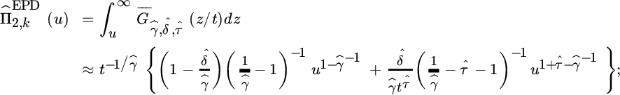
- Generalized Pareto fit:

When u < t, we have from (4.3.43) that

Note that Π(u) = 0 for u ≥ T and Π(u) = Π(tl) + (tl − u) for u ≤ tl. For the mixed Erlang distribution we get

with

and, assuming that rn = n, n = 1, …, M,


Figure 4.24 MTPL data for Company A: XL pure premium Π(u) based on ME‐Pa fit taking interval censoring into account. Comparison with the result when the upper bounds are ignored (right censoring) and when the premium is based on the ultimates.
Of course the estimation of Π(u) can be extended to a regression context. For instance, when u = u(x) is larger than a threshold function μ(x) of a one‐dimensional covariate x, and using the GPD modelling approach, one obtains for ![]()
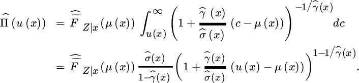
The result of this procedure based on the GPD regression fit for the storm claim data of Upper Austria, with GPD(0.445, e−7.2+0.046w, 0), is shown in Figure 4.25.

Figure 4.25 Austrian storm claim data: XL pure premium Π(exp(0.001w)) for Upper Austria based based on a GPD regression fit with the wind index W as covariate.
4.7 Further Case Studies
We end this chapter by analysing the case studies on flood risk and earthquake risk which were introduced in Chapter 1.
- Flood risk. Here we model the aggregate annual loss data introduced in Section 1.3.4 (given as a percentage of the building value) for Germany and the UK. All presented derivative plots for Germany in Figure 4.27 based on the Pareto, log‐normal, and Weibull QQ‐plots ultimately are decreasing, while for the UK in Figure 4.26 the decrease in the Weibull derivative plot is small and this plot is closest to being constant when
 . The systematic decrease in the different estimators of γ with increasing threshold, together with the P‐values of the TB test for upper‐truncation does indicate some evidence for a truncated Pareto tail. Indeed, for both countries the truncated Pareto model fits well. The estimates
  of the right truncation point T are situated around 0.25 for the UK and 0.35 for Germany. However, for the UK data, a Weibull fit provides a valid alternative.
 - Earthquake risk. We consider recent magnitude data of the 200 largest earthquakes in the Groningen area (the Netherlands) which are caused by gas extraction. In Figure 4.28 (top left), we present the exponential QQ‐plot. A linear pattern is visible for a large section of the magnitudes data, while some concave curvature appears at the largest values. Along the Gutenberg–Richter (1956) law the magnitudes of independent earthquakes are drawn from a doubly truncated exponential distributionKijko and Singh [487] provide a review of the vast literature on estimating the maximum possible magnitude TM. The energy E released by earthquakes, expressed in megaJoules, relates to the magnitude M by
 When transforming the magnitude data back to the energy scale, the Gutenberg–Richter model predicts a truncated Pareto tail. In Figure 4.28, plotting the Hill estimates we observe a systematic decrease with decreasing k, while the moment and ML‐GPD estimators tend to − 1 near k = 1. The estimates of
 stay rather stable at a level
  . The P‐values of the TB test for upper‐truncation are boundary significant at significance level 0.05 for k ∈ (30, 70). The amount of truncation is estimated around
  . The goodness of fit of the truncated Pareto fit is illustrated on the Pareto QQ‐plot of the energy data where the truncated Pareto‐model is fitted based on the top 50 values. The maximum magnitude
  is then estimated at 3.75 for the Groningen area.


Figure 4.26 UK flood loss data: mean excess plot (xn−k, n, ek, n) (top left); Hill plot  (top right); log‐normal derivative plot
  (second line left); Weibull derivative plot
  (second line right); γ estimates (third line left); P‐values of TB test (third line right); endpoint estimates
  (bottom left); Pareto QQ‐plot with truncated Pareto fit (full line) and Pareto fit (dashed line) (bottom right).

Figure 4.27 Flood loss data Germany: mean excess plot (xn−k, n, ek, n) (top left); Hill plot  (top right); log‐normal derivative plot
  (second line left); Weibull derivative plot
  (second line right); γ estimates (third line left); P‐values of TB test (third line right); endpoint estimates
  (bottom left); Pareto QQ‐plot with truncated Pareto fit (full line), and Pareto fit (dashed line) (bottom right).

Figure 4.28 Earthquake magnitude data from Groningen area. Exponential QQ‐plot based on magnitudes (top left); estimates of γ (top right); TB P‐value plot (middle left);  estimates (middle right); Pareto QQ‐plot of energy values with truncated Pareto fit (bottom right); estimates of maximum magnitude
  (bottom right).
4.8 Notes and Bibliography
In case of the Gumbel domain of attraction with γ = 0, EVA based on fitting a generalized Pareto distribution to POT values is known to exhibit slow convergence rates in many cases. To this end more specific models have been proposed, for example El Methni et al. [320] and De Valk and Cai [262].
In the last few decades some papers have appeared concerning robust estimation methods. Robust methods can improve the quality of extreme value data analysis by providing information on influential observations, deviating substructures and possible mis‐specification of a model while guaranteeing good statistical properties over a whole set of underlying distributions around the assumed one. On the other hand an EVA precisely is performed to consider and emphasize the role of extremes. Hence in a risk management context it can hardly be the purpose to delete the most extreme observations when they were correctly reported. Robust and non‐robust estimators then yield different scenarios for risk assessment should be compared. An interesting discussion on this can be found in Dell’Aquila and Embrechts [270].
EVA is an active field of research. A notable recent contribution is Naveau et al. [587], which gives an alternative to splicing methods in order to produce full models in a hydrological context. In De Valk [261] and Guillou et al. [415], some further new modelling approaches in the multivariate case are introduced.
A Bayesian approach to estimate the total cost of claims in XL reinsurance has been covered in Hesselager [441]. For the estimation of the Pareto index in XL treaties, see Reiss et al. [644]. Leadbetter [529] studied the connection between tail inference and high‐level exceedance modelling, which is relevant for the XL case. Examples of early statistical analyses of large fire losses are Ramachandran [639], Ramlau‐Hansen [640], and Corradin et al. [227]. Resnick [646] also studied the Danish fire insurance data set. Data for coverages of homes are analyzed in Grace et al. [404]. For glass losses, see Ramlau‐Hansen [640]. Property reinsurance for the USA is covered in Gogol [394], for example.