
CHAPTER 10
RESOURCE ALLOCATION IN MULTI-TIER NETWORKS WITH COGNITIVE SMALL CELLS
10.1 INTRODUCTION
For small cells to succeed, cognition is expected to be a necessary feature that should be implemented in all types of small cells for their efficient operation with limited centralized control. This cognition will enable the small cells to have the SON capabilities (e.g., self-configuration, self-optimization, and self-healing) which will result in low capital expenditure (CAPEX) and operation expenditure (OPEX) for the network operators. For cognitive small cells, the corresponding BSs, that is, SBSs, will be capable of monitoring the surrounding environment, locating major interference sources and avoiding them by opportunistically accessing the orthogonal channels. The concepts of dynamic spectrum access used in cognitive radio can be applied to multi-tier networks with small cells to tackle some of the major challenges of small cell deployment which include the following: limited centralized control, unplanned and massive deployment, limited transmission powers of small cells and huge transmission power gap between macrocells and small cells, coexistence and efficient operation, and requirement for self-organizing capability. Cognitive SBSs should be able to distributively monitor the spectrum and avoid major interference sources by opportunistically accessing the radio channels so that the interference from nearby MBSs and closed access SBSs is avoided. The closed access SBSs (e.g., closed access femtocells) can also be cognitive to avoid using the same frequency band used by nearby MBSs, so that the macro users are not affected by the interference from the nearby closed access SBSs.
The resource allocation in a multi-tier network and the network performance are closely related to the off-loading technique used to divide the traffic load among the different network tiers. In this chapter, we will discuss how to evaluate the share that each network tier serves from the complete set of users and how to optimize the design parameters to off-load users from one network tier to another. We are concerned with traffic off-loading via access network connectivity. That is, we design the multi-tier network such that the users are more oriented to connect to (i.e., associate with) the designated network tier, or transmit more of their traffic via the designated network tier. For instance, traffic off-loading to the small cell tier implies that users prefer to connect to the SBSs, and hence, the percentage of the traffic communicated via the small cell tier is increased. Off-loading users to the small cells has two merits, one from the access network and the other from the core network point of view. For the access network, with off-loading, we can decrease the congestion in the macro access network and achieve the optimal balance between the users served by each access network tier. In this way, the blocking probability in the macro tier due to the unavailability of radio resources can be minimized and the utilization of wireless resources can be improved. For the core network, since some small cells (such as femtocells) are IP-backhauled, traffic is off-loaded to the IP network, and therefore, the congestion in the service providers core network decreases.
We will investigate and quantify the off-loading efficiency for three major off-loading techniques in a two-tier network, namely, off-loading via power control, off-loading via increasing the intensity of SBSs, and off-loading via biasing [1]. The concept of biasing was suggested in [2] to motivate the users to associate with the SBSs (femtocells in their case) even if the strongest signal is received from the nearest MBS. The biasing can be viewed as a virtual increase in the relative trans-mission power of the SBSs to extend their range [3,4]. In [2], it was assumed that the SBSs and the MBSs aggressively use the same channel. Hence, due to the severe interference from the geographically nearest MBS, biasing off-loads users to the small cell tier at the expense of increased outage probability. However, as will be discussed later, if the SBSs are cognitive, severe interference from the nearby MBS will be avoided and off-loading via biasing would not increase the outage probability of small cell users [5–7]. The off-loading efficiency of macro users to small cells can be quantified through the tier association probability. The tier association probability is the probability that a generic user, located at a generic location is associated with a given network tier (i.e., small cell network tier or macro network tier). This is based on the fact that each user associates (connects) with the network entity (i.e., MBS or SBS) which provides the highest instantaneous signal power.
Since the deployment of small cells brings topological randomness in the network, the traditional grid-based modeling approach used for single-tier cellular networks may not be suitable to model and analyze such multi-tier networks. Recently, a new modeling approach based on Stochastic Geometry has been used to model and analyze multi-tier cellular networks [8]. In the next section, basics of the stochastic geometry-based modeling will be discussed in the context of cellular wireless networks.
10.2 BACKGROUND
In wireless communications, the signal power decays with the distance between the transmitter and the receiver according to the power law, that is,
where Pt(x) is the transmission power from a transmitter located at ![]() ,
, ![]() is the receiver position, hxy is a random variable accounting for the random channel (power) gain between the two locations x and y,
is the receiver position, hxy is a random variable accounting for the random channel (power) gain between the two locations x and y, ![]() is the Euclidean norm, A is a propagation constant, and η is the path-loss exponent.1 Although (10.1) holds for any number of dimensions, the dimensions d = 1, 2, and 3 are of primary interest due to their physical interpretations. Due to the distance-dependent signal power decay along with the shared nature of the wireless medium, the network geometry has a significant impact on the performance of wireless networks. That is, the position of a test receiver with respect to its serving network entity strongly affects the useful signal. On the other hand, the position of the test receiver with respect to other network entities that are simultaneously using the same channel affects the interference signal seen by the test receiver. Therefore, the network geometry has a significant impact on the SINR experienced by the receivers.
is the Euclidean norm, A is a propagation constant, and η is the path-loss exponent.1 Although (10.1) holds for any number of dimensions, the dimensions d = 1, 2, and 3 are of primary interest due to their physical interpretations. Due to the distance-dependent signal power decay along with the shared nature of the wireless medium, the network geometry has a significant impact on the performance of wireless networks. That is, the position of a test receiver with respect to its serving network entity strongly affects the useful signal. On the other hand, the position of the test receiver with respect to other network entities that are simultaneously using the same channel affects the interference signal seen by the test receiver. Therefore, the network geometry has a significant impact on the SINR experienced by the receivers.
The SINR for a test receiver in the network (Figure 10.1) can be calculated as follows:
(10.2) ![]()
where y is the location of the test receiver, x0 is the location of the test transmitter (desired transmitter), ![]() is the set of interferers (active transmitters using the same channel as that of the test transmitter), and W is the noise power. The term
is the set of interferers (active transmitters using the same channel as that of the test transmitter), and W is the noise power. The term ![]() is the aggregate interference power at the test receiver. Note that according to the network model,
is the aggregate interference power at the test receiver. Note that according to the network model, ![]() can be finite or infinite and the locations and the intensity of the interferers depend on the network characteristics (e.g., network topology and number of channels) and MAC layer protocol (e.g., ALOHA, CSMA, TDMA, and CDMA). At a generic time instant, the SINR experienced by each receiver depends on its location, the positions of the interference sources as well as the instantaneous channel gains. Hence, the SINR is a random variable that strongly depends on the network geometry and significantly varies from one receiver to another and from one time instant to another.
can be finite or infinite and the locations and the intensity of the interferers depend on the network characteristics (e.g., network topology and number of channels) and MAC layer protocol (e.g., ALOHA, CSMA, TDMA, and CDMA). At a generic time instant, the SINR experienced by each receiver depends on its location, the positions of the interference sources as well as the instantaneous channel gains. Hence, the SINR is a random variable that strongly depends on the network geometry and significantly varies from one receiver to another and from one time instant to another.
FIGURE 10.1 Test receiver in a two-tier network.

FIGURE 10.2 (a) The network modeled as a weighted Voronoi tessellation (b) the network modeled as a superposition of two independent Voronoi tessellations (the diamond dots with the dashed Voronoi represent the macro network tier) (© [2012] IEEE).

For a generic node in the network, the aggregate interference,![]() is a stochastic process that depends on the locations of the interferers captured by the point process
is a stochastic process that depends on the locations of the interferers captured by the point process ![]() and the random channel gains hxy. Note that
and the random channel gains hxy. Note that ![]() is defined by the network properties and the MAC layer. Generally, there is no known expression for the pdf of the aggregate interference in large-scale networks. Hence, the aggregate interference is usually characterized using the LT of the pdf (or equivalently its CF or moment generation function [MGF]). The LT of the aggregate interference is given by
is defined by the network properties and the MAC layer. Generally, there is no known expression for the pdf of the aggregate interference in large-scale networks. Hence, the aggregate interference is usually characterized using the LT of the pdf (or equivalently its CF or moment generation function [MGF]). The LT of the aggregate interference is given by
(10.3) ![]()
With the LT, CF, or MGF, we are able to generate the moment (if they exist) of the aggregate interference as ![]() , where
, where ![]() is the nth derivative of
is the nth derivative of ![]() . In the general case, it is not possible to derive the exact performance metrics (e.g., outage probability, transmission capacity, and average achievable rate) from the LT, CF, or the MGF.
. In the general case, it is not possible to derive the exact performance metrics (e.g., outage probability, transmission capacity, and average achievable rate) from the LT, CF, or the MGF.
Stochastic geometry is a mathematical tool that provides spatial averages, that is, averages taken over large number of nodes at different locations and over many network realizations [10], for the quantities of interest (e.g., interference, SINR, outage probability, and achieved data rate) [11]. In other words, the stochastic geometry averages over all network topologies seen from a generic node weighted by their probability of occurrence [12, 13].
Due to the variation of capacity demand across the network, both single-tier and multi-tier cellular networks are characterized by their random topologies [14,15]. In this chapter, we will use stochastic geometry for modeling and analysis of a two-tier network. Stochastic geometry is a very powerful tool to model and analyze networks with random topologies, where point processes are used to model the spatial distribution for the network entities [11, 16]. Recently, it has been shown that stochastic geometry provides a tractable yet accurate modeling for cellular networks as well as multi-tier networks [14, 15], where point processes are used to model the spatial distribution of the network entities. The PPP is the most popular and well-understood point process in the literature due to its simplicity and tractability.
A point process in ![]() is a PPP if and only if the number of points inside a bounded Borel set
is a PPP if and only if the number of points inside a bounded Borel set ![]() has a Poisson distribution with a mean directly proportional to the Lebesgue measure of B, and the numbers of points in disjoint Borel sets are independent [16]. That is, the PPP assumes that the positions of the points are uncorrelated. Although the assumption that the positions of the MBSs are uncorrelated is unrealistic, it was shown in [14] that the PPP assumption for the spatial location of the MBSs provides a lower bound on coverage probability (i.e., the complement of the outage probability) and the average achievable rate that is as much tight as the upper bound provided by the idealized grid-based model traditionally used for modeling cellular networks. In [15], it was shown that the PPP assumption is accurate to within 1–2 dB of the performance of an actual LTE network overlaid by heterogeneous tiers modeled as PPP.
has a Poisson distribution with a mean directly proportional to the Lebesgue measure of B, and the numbers of points in disjoint Borel sets are independent [16]. That is, the PPP assumes that the positions of the points are uncorrelated. Although the assumption that the positions of the MBSs are uncorrelated is unrealistic, it was shown in [14] that the PPP assumption for the spatial location of the MBSs provides a lower bound on coverage probability (i.e., the complement of the outage probability) and the average achievable rate that is as much tight as the upper bound provided by the idealized grid-based model traditionally used for modeling cellular networks. In [15], it was shown that the PPP assumption is accurate to within 1–2 dB of the performance of an actual LTE network overlaid by heterogeneous tiers modeled as PPP.
Definition 10.1 (Definition 1).(Poisson point process (PPP)): A point process ![]() is a PPP if and only if the number of points inside any compact set
is a PPP if and only if the number of points inside any compact set ![]() is a Poisson random variable, and the numbers of points in disjoint sets are independent.
is a Poisson random variable, and the numbers of points in disjoint sets are independent.
When the locations of the interferers are modeled as a PPP, the LT of the pdf of aggregate interference can be determined using the following lemma.
Lemma10.1 Following (sec. 3.7.1, [17]), in a Rayleigh fading environment, the LT of the pdf of the aggregate interference measured at the origin from a PPP with intensity λ and existing outside ![]() is given by
is given by
(10.4) ![]()
Subsequently, the LT of the pdf of aggregate interference above can be used to obtain performance measures such as outage probability, network coverage, and data rate. Under Rayleigh fading, the outage probability for a test receiver can be obtained as follows. Without loss of generality, let ![]() be the constant distance between the transmitter and the test receiver,
be the constant distance between the transmitter and the test receiver, ![]() be the channel power gain of the useful link, then we have
be the channel power gain of the useful link, then we have
(10.5) 
where the expectation in (i) is with respect to both the point process and the channel gains between the interference sources and the test receiver, and ![]() is a constant.
is a constant.
With channel sensing-based dynamic spectrum access capability, the spatial distribution of the simultaneously active small cells (i.e., cognitive small cells), can be modeled by a Matérn hard core point process (HCPP) [10,16,18–20]. A Matérn HCPP is a repulsive point process where no two points can coexist if their distance is less than the hard core radius rh. The Matérn HCPP is derived from a PPP via dependent thinning. The dependent thinning is applied in two steps. First, an independent uniformly distributed time mark is applied to the PPP. Then, a point is chosen to be in the Matérn HCPP if and only if it has the lowest mark in its contention domain. The contention domain of a point is defined by a circle of radius rh around that point.
Definition 10.2 (Definition 2).(HCPP): An HCPP is a repulsive point process where no two points of the process coexist with a separating distance less than a predefined hard core parameter rh. A point process ![]() is an HCPP if and only if
is an HCPP if and only if ![]() ,
, ![]() ,
, ![]() , where
, where ![]() is a predefined hard core parameter.
is a predefined hard core parameter.
The LT of the pdf of the aggregate interference due to an HCPP has always been approximated by the LT of the pdf of the aggregate interference due to the PPP with the same intensity but existing outside the contention domain of the test transmitter [19–22]. The rationale behind this approximation is that the main factors affecting the aggregate interference are the number of interferers and their locations with respect to the test node. However, the locations of the interferers with respect to each other have minimal effect on the interference at the test node. The number of interferers has been captured in the calculation of the intensity of the HCPP and the locations of the interferers with respect to the test receiver have been captured by conditioning on having the PPP outside the contention domain of the test transmitter.
10.3 ANALYSIS OF TIER-ASSOCIATION PROBABILITY
10.3.1 System Model and Assumptions
In multi-tier cellular networks, the coverage of each network entity depends on its type (i.e., a macrocell base station [MBS], microcell base station [MiBS], picocell base station [PiBS], or a femto access point [FAP]) and the network geometry (i.e., its location with respect to other network entities). That is, assuming that each user will associate with (is covered by) the network entity that provides the highest signal power, the coverage of each network entity will depend on its transmission power as well as the relative positions of the neighboring network entities and their transmission powers. For instance, if two MBSs have the same transmission power, a line bisecting the distance between them will separate their coverage areas. However, for an MBS with 100 times higher transmission power than an SBS, a line dividing the distance between them with a ratio of 100:1 will separate their coverage areas, and so on. If all tiers are modeled via independent homogenous PPPs, due to the high variation of the transmission power of BSs belonging to different tiers, the multi-tier cellular network coverage will constitute a weighted Voronoi tessellation. The weighted Voronoi tessellation is the planar graph constructed by bisecting the distances between the points of a PPP according to the ratio between their weights, where the weights correspond to the transmission powers of the network entities.
Let us consider a two-tier network where MBSs overlaid by FAPs. As the FAPs are deployed randomly according to the end user requirements without any network planning from the cellular network provider. Then, we assume that the two network tiers are independent and each is represented by an independent PPP. That is, the MBSs are spatially distributed according to the PPP ![]() with intensity
with intensity ![]() where bi is the location of the ith MBS. The FAPs are spatially distributed according to the PPP
where bi is the location of the ith MBS. The FAPs are spatially distributed according to the PPP ![]() with intensity
with intensity ![]() where ai denotes the location of the ith FAP. The coverage of each tier forms a Voronoi tessellation [16]. Due to the difference in transmission powers between the MBS and the FAPs, the network model can be represented by a weighted Voronoi tessellation as shown in Figure 10.2(a) [15]. However, since the two tiers are independent, the network model can be considered as a superposition of two independent Voronoi tessellations, one for the MBSs and the other for FAPs as shown in Figure 10.2(b). By construction, the Voronoi cells belonging to the same tier do not intersect. Hence, each user will fall in an intersection between two Voronoi cells belonging to different tiers (i.e., one of an MBS and the other of a FAP). Based on the radio signal strength (RSS) level, each user will be associated to either the MBS or the FAP of the Voronoi cells covering the user. In particular, the user will always be connected to the geographically nearest MBS or to the geographically nearest FAP.
where ai denotes the location of the ith FAP. The coverage of each tier forms a Voronoi tessellation [16]. Due to the difference in transmission powers between the MBS and the FAPs, the network model can be represented by a weighted Voronoi tessellation as shown in Figure 10.2(a) [15]. However, since the two tiers are independent, the network model can be considered as a superposition of two independent Voronoi tessellations, one for the MBSs and the other for FAPs as shown in Figure 10.2(b). By construction, the Voronoi cells belonging to the same tier do not intersect. Hence, each user will fall in an intersection between two Voronoi cells belonging to different tiers (i.e., one of an MBS and the other of a FAP). Based on the radio signal strength (RSS) level, each user will be associated to either the MBS or the FAP of the Voronoi cells covering the user. In particular, the user will always be connected to the geographically nearest MBS or to the geographically nearest FAP.
The UEs are spatially distributed according to an independent PPP ![]() with intensity
with intensity ![]() . We consider a general power-law path-loss model in which the signal power decays at the rate
. We consider a general power-law path-loss model in which the signal power decays at the rate ![]() with the distance r, where
with the distance r, where ![]() is the path-loss exponent. To obtain general results, Nakagami-m fading environment is assumed where m=1 represents Rayleigh fading and
is the path-loss exponent. To obtain general results, Nakagami-m fading environment is assumed where m=1 represents Rayleigh fading and ![]() represents deterministic path-loss. In this chapter, we will use the notation
represents deterministic path-loss. In this chapter, we will use the notation ![]() to denote the channel (power) gain between the test user and FAP ai, and the notation
to denote the channel (power) gain between the test user and FAP ai, and the notation ![]() to denote the channel (power) gain between the test user and the MBS bi. The channel power gains have the gamma pdf,
to denote the channel (power) gain between the test user and the MBS bi. The channel power gains have the gamma pdf, ![]() and cdf
and cdf ![]() , where
, where ![]() is the gamma function,
is the gamma function, ![]() is the upper incomplete gamma function, m is the shape parameter and μ is the scaling parameter.
is the upper incomplete gamma function, m is the shape parameter and μ is the scaling parameter.
10.3.2 Tier Association Probability
Based on the instantaneous RSS level, each user will associate with either the MBS or the FAP of the Voronoi cells covering that user. Therefore, each user will only have two candidate network entities to associate with, the geographically nearest MBS and the geographically nearest FAP. Without any loss of generality, the analysis is conducted on a typical user located at the origin. According to Slivnyak’s theorem [16], conditioning on having a user at the origin does not change the statistical properties of the coexisting PPPs. Hence, the analysis holds for any generic user located at a generic location [14, 15]. The association probability to the femto network tier and the macro network tier can be obtained from the following lemma.
Lemma 10.2 In a Nakagami-m fading environment, the probability that a generic user is associated with the femto network is given by
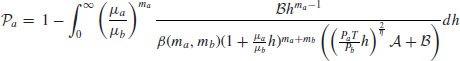
where ![]() is the beta function, and
is the beta function, and ![]() is a biasing factor to bias users to associate with the femto network tier. The probability that a generic user is associated with the macro network is given by
is a biasing factor to bias users to associate with the femto network tier. The probability that a generic user is associated with the macro network is given by
(10.7) 
Proof: Let ![]() ,
, ![]() be the distance from the user located at the origin to the nearest FAP, and
be the distance from the user located at the origin to the nearest FAP, and ![]() ,
, ![]() be the distance from the user located at the origin to the nearest MBS. Then, the cdf of the distance Ra can be easily derived for the PPP null probability as follows [14, 16]:
be the distance from the user located at the origin to the nearest MBS. Then, the cdf of the distance Ra can be easily derived for the PPP null probability as follows [14, 16]:
(10.8) ![]()
Differentiating the cdf of Ra, the pdf of Ra is obtained as follows:
(10.9) ![]()
Similarly, the pdf of Rb is obtained as
(10.10) ![]()
From the system model, we know that there are only two candidate network entities for a generic user to associate with (the nearest MBS and the nearest FAP). Hence, the probability that a test user ui located at the origin associates with the nearest FAP is given by the probability that the nearest FAP signal power (with biasing) is greater than the received signal power from the nearest MBS.

where ![]() and
and ![]() . The pdf of ha/b is given by
. The pdf of ha/b is given by
The cdf of Ra/b is obtained as

Substituting (10.12) and (10.13) in (10.11), Equation (10.6) is obtained and the lemma is proved. ![]()
The tier association probability can be directly interpreted as the probability that a generic user will associate with one of the two network tiers at a generic time instant. Also, the association probability can be viewed as the percentage of time that a generic user will be connected to a given network tier, or as the percent of traffic that a user communicates through a certain network tier, or as the share that each network tier serves from the complete set of users, or as the portion of the plane which each tier is serving. The off-loading of users can be quantified by using any of these different interpretations for the tier association probability.
From (10.6), it can be shown that the femto tier association probability (and hence off-loading of the users) can be controlled via manipulating three main parameters, namely, the relative transmission power of FAPs, the relative intensity of FAPs by deploying more FAPs, and the biasing factor. The biasing factor is suggested in [2] to bias the users to associate with the FAPs even if the strongest signal is received from the nearest MBS. The biasing can be viewed as a virtual increase in the relative transmission power of FAPs. It is shown in [2] that biasing off-loads users to the femto tier, and hence increases the users’ minimum achievable rate at the expense of increased outage probability. The relative channel gain of the users toward the FAPs has also a fundamental impact on the association probability. FAPs are usually deployed at indoor locations. As a result, there will be favorable channel gains toward the FAPs in comparison with the channel gains toward the MBS. The favorable channel gains toward the FAPs also result in a natural biasing of the users to associate with the femto tier as will be evidenced from the numerical results.
Another important quantity of interest is the number of users associated with each network entity. From the interpretations of the tier association probability and the fact that independently thinning a PPP produces another PPP [16], the PPP representing the complete set of users ![]() can be divided into two independent PPPs:
can be divided into two independent PPPs: ![]() with intensity
with intensity ![]() and
and ![]() with intensity
with intensity ![]() which denote, respectively, the PPP for the users associated to the FAPs and the users associated to the MBSs. As shown in (10.6), off-loading to the FAPs can be achieved via increasing the intensity of the FAPs. However, increasing the intensity of the FAPs will decrease the number of users associated with each FAP. In order to avoid having lots of idle FAPs (i.e., FAPs without any associated users) we have to derive the number of users associated with a generic FAP, which is a discrete random variable. The distribution of the number of users associated to a generic FAP is given by the following lemma.
which denote, respectively, the PPP for the users associated to the FAPs and the users associated to the MBSs. As shown in (10.6), off-loading to the FAPs can be achieved via increasing the intensity of the FAPs. However, increasing the intensity of the FAPs will decrease the number of users associated with each FAP. In order to avoid having lots of idle FAPs (i.e., FAPs without any associated users) we have to derive the number of users associated with a generic FAP, which is a discrete random variable. The distribution of the number of users associated to a generic FAP is given by the following lemma.
Lemma 10.3 Given that the intensity of users associated with the femto network tier is ![]() and that each femto user is associated with its geographically nearest FAP, the distribution of the number of users associated with each FAP is given by:
and that each femto user is associated with its geographically nearest FAP, the distribution of the number of users associated with each FAP is given by:
(10.14) ![]()
where c=3.575 is a constant.
Proof: Conditioning on a Voronoi cell area V, the number of femto users Nf in that Voronoi cell is a Poisson random variable with the probability mass function (pmf) given by
Note that in (10.15) we account only for femto users by considering ![]() . The Voronoi cell area V of the FAPs’ Voronoi tessellation is a random variable that follows the gamma distribution
. The Voronoi cell area V of the FAPs’ Voronoi tessellation is a random variable that follows the gamma distribution ![]() ,
, ![]() , where c=3.575 is a constant defined for the Voronoi tessellation in the
, where c=3.575 is a constant defined for the Voronoi tessellation in the ![]() . Therefore, the unconditional pmf of Nf is given by
. Therefore, the unconditional pmf of Nf is given by

where in ![]() , the integration C evaluates to 1 because it is an integration of a gamma pdf over its entire support domain. We will denote the cdf of Nv by
, the integration C evaluates to 1 because it is an integration of a gamma pdf over its entire support domain. We will denote the cdf of Nv by ![]() and it is given by
and it is given by
(10.16) ![]()
![]()
10.3.3 Numerical Results
Figure 10.3 shows the effect of the different system parameters on the off-loading in a two-tier network. Let ![]() and
and ![]() denote, respectively, the intensities of SBSs and the MBSs. In Figure 10.3, we start at
denote, respectively, the intensities of SBSs and the MBSs. In Figure 10.3, we start at ![]() ,
, ![]() , and
, and ![]() . Then according to the tested off-loading technique, we increase the corresponding off-loading parameter until it reaches 10 times of its initial value. For instance, when testing the off-loading via power control or biasing, we start at
. Then according to the tested off-loading technique, we increase the corresponding off-loading parameter until it reaches 10 times of its initial value. For instance, when testing the off-loading via power control or biasing, we start at ![]() . Then we increase PsT until we reach
. Then we increase PsT until we reach ![]() (i.e., 10 times of its original value). We do the same for off-loading via increasing the intensity. That is, we start at
(i.e., 10 times of its original value). We do the same for off-loading via increasing the intensity. That is, we start at ![]() , then we increase
, then we increase ![]() until we reach
until we reach ![]() . Finally, for the natural off-loading due to the favorable channel gain, we start at
. Finally, for the natural off-loading due to the favorable channel gain, we start at ![]() , then we increase
, then we increase ![]() until we reach
until we reach ![]() .
.
FIGURE 10.3 The effect of each offloading technique on the tier association probability (© [2013] IEEE).

Figure 10.3 shows that increasing the intensity of the SBSs has the greatest impact on the tier association probability. On the other hand, the power control has the least impact on the tier association probability. For instance, increasing the intensity of SBSs by 5 times increases the small cell tier association probability by 2.92 times. However, increasing the transmission power of SBSs by 5 times increases the small cell tier association probability by only 1.7 times. For more numerical results, refer to [23]. It is worth mentioning that the presented paradigm can be easily extended to evaluate the share of each network tier in a multi-tier network and quantify the off-loading achieved by manipulating different design parameters.
10.4 COGNITION TECHNIQUES FOR SMALL CELLS
The share that each network serves from the complete set of users is not the only important parameter that affects the performance of a multi-tier network. Even more important is how efficiently the users are served within each network tier. As discussed before, mutual interference is the most performance limiting parameter in multi-tier networks and it is infeasible to use traditional centralized techniques to coordinate the spectrum access by a large number of SBSs, allocate their resources, and limit the mutual interference. In this section, we discuss distributed spectrum access via cognitive radio, its design, and its effect on the network performance. A cognitive SBS will not access a channel unless the interference received on that channel from any other network entities is less than the spectrum sensing threshold.
Due to the distance-dependent signal power decay, the spectrum sensing threshold defines an area where no interference source exists (Figure 10.4). That is, a channel used by a network entity (i.e., an MBS or an SBS) located at ![]() can be reused by a cognitive SBS located at
can be reused by a cognitive SBS located at ![]() if and only if
if and only if
FIGURE 10.4 Spectrum sensing range for cognitive small cells (rsa, rsb are spectrum sensing range with respect to other small cells and the macrocell, respectively).

where h(x, y) denotes the random channel gain between the two locations x and y, Ptx is the transmission power of the network entity located at x, γ is the spectrum sensing threshold, ![]() is the Euclidean norm, and η is the path-loss exponent. It can be seen from (10.17) that the spectrum sensing threshold is the design parameter that controls the minimum frequency reuse distance
is the Euclidean norm, and η is the path-loss exponent. It can be seen from (10.17) that the spectrum sensing threshold is the design parameter that controls the minimum frequency reuse distance ![]() , and hence the spatial reuse efficiency. The higher the value of the spectrum sensing threshold, the lower is the frequency reuse distance and the more aggressive will be the cognitive SBSs in accessing the channels. Hence, the mutual interference increases leading to a higher outage probability, and vice versa. Therefore, there is a trade-off between the spatial frequency reuse efficiency and the outage probability that can be optimized by carefully tuning the spectrum sensing threshold.
, and hence the spatial reuse efficiency. The higher the value of the spectrum sensing threshold, the lower is the frequency reuse distance and the more aggressive will be the cognitive SBSs in accessing the channels. Hence, the mutual interference increases leading to a higher outage probability, and vice versa. Therefore, there is a trade-off between the spatial frequency reuse efficiency and the outage probability that can be optimized by carefully tuning the spectrum sensing threshold.
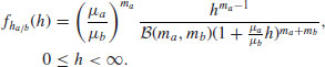
Note that the spatial frequency reuse efficiency also translates to an outage probability due to the opportunistic spectrum access by the SBSs. In other words, a cognitive SBS will not access a channel which is being used by the nearby MBS and the SBSs (such a scheme is referred to as Scheme-1 here); hence, unavailability of radio channels may lead to outage. Spectrum access for cognitive SBS can be implemented in a way similar to the traditional slotted carrier-sense multiple access (CSMA). For example, each time slot can be divided into three main parts (Figure 10.5(a)). In the first part, each cognitive SBS senses the available spectrum to detect the channels which are not being used by the MBS. Then, in the second part, each cognitive SBS contends to access one of the available channels (e.g., using a random backoff process while persistently sensing the channel). Finally, in the third part, if the sensed channel is available during the entire backoff duration (i.e., not used by a nearby SBS), the cognitive SBS transmits on that channel for the rest of the time slot. Otherwise, the cognitive SBS is considered to be in outage due to channel unavailability.
FIGURE 10.5 Distributed channel access by SBSs: (a) Scheme-1 and (b) Scheme-2 (© [2013] IEEE).
For DL transmission, the total outage probability for a small cell user can be expressed as follows [23]:
where SINR is the signal-to-interference-plus-noise ratio and β is the threshold defined for correct signal reception. Note that using stochastic geometry, Pout can be obtained in a systematic manner. According to (10.18), the outage could be due to channel unavailability for opportunistic access and/or due to SINR violation (i.e., resulting from aggregate interference). As discussed above, both of these outages are functions of the spectrum sensing threshold. Increasing the spectrum sensing threshold decreases the frequency reuse distance and increases the opportunistic channel access. However, this increases the aggregate interference and hence the SINR outage. On the other hand, decreasing the sensing threshold will increase the frequency reuse distance and hence decrease the aggregate interference, and therefore, decrease the SINR outage. However, the outage due to opportunistic channel access may increase due to increased contention resulting from higher number of SBSs within the frequency reuse distance.
For a given spectrum sensing threshold, since the opportunistic spectrum access performance of the small cells will be deteriorated when the intensity of the deployed SBSs is high, introducing spectrum awareness at an SBS with respect to the spectrum usage at the other SBSs may not be the best solution. Instead, cognition can be introduced only with respect to the macro-tier. That is, each SBS senses the spectrum to locate the channels which are not used by the MBS and uses any of them without considering the other SBSs (Scheme-2 in Figure 10.5(b)). In this case, for example, each time slot can be divided into two main parts. In the first part, each cognitive SBS senses the available spectrum to detect the channels which are not used by the MBS. Then, in the second part, each cognitive SBS selects one of the available channels and transmits in that channel. Hence, channels will be aggressively used in the small cell tier to increase their opportunistic spectrum access performance at the expense of higher mutual interference in the small cell tier.
Figure 10.6 shows the performance gain in the outage probability obtained by introducing cognition to the SBSs and to compare these two different cognition techniques. Figure 10.6(a) shows that there exists an optimal spectrum sensing threshold that depends on the network parameters and the cognition technique. A higher value of spectrum sensing threshold results in shorter frequency reuse distances and more spectrum opportunities. However, the aggregate interference increases and dominates the outage probability. This results in a degraded outage performance. For very high values of spectrum sensing threshold, the cognitive SBSs become very aggressive and their performance matches with that of the non-cognitive SBSs. On the other hand, lower values of spectrum sensing threshold result in higher frequency reuse distance and lower aggregate interference; however, the opportunistic spectrum access probability decreases and dominates the outage probability. Figure 10.6(b) shows the decomposed outage probability for both the cognition techniques. As shown in the figure, for Scheme-1, the decreased SINR outage probability is wasted by the outage probability due to the channel unavailability. On the other hand, the degraded SINR outage probability of Scheme-2 is balanced by the improved spectrum access probability. Importantly, Figure 10.6 shows that cognition is an important feature that can significantly enhance the multi-tier performance and that introducing cognition with respect to the macro-tier only is more beneficial than introducing cognition with respect to both the network tiers. This is due to the massive deployment of the small cells along with the uncoordinated access (i.e., contention) among the coexisting SBSs.
FIGURE 10.6 (a) The total outage probability of small cell users versus spectrum sensing threshold for cognitive techniques for Pb=5 W, Ps=100 dBm, ![]() MBS/km2,
MBS/km2, ![]() SBS/km2,
SBS/km2, ![]() ,
, ![]() , and
, and ![]() and (b) for the same parameters, the decomposed outage probability of small cell users versus spectrum sensing threshold for both the cognitive techniques (© [2013] IEEE).
and (b) for the same parameters, the decomposed outage probability of small cell users versus spectrum sensing threshold for both the cognitive techniques (© [2013] IEEE).

10.5 DISCUSSIONS AND FUTURE RESEARCH DIRECTIONS
The main design challenge for multi-tier networks arises due to the complicated relationship between the design parameters and the performance metrics due to the coexistence of multiple network tiers. To elaborate, we give the following example. Increasing the intensity of the deployed SBSs achieves better performance from higher off-loading from the macro network tier to the small cell tier. Hence, the number of users served per MBS as well as the number of channels used per MBS decreases. Therefore, more channels are available for the SBSs to contend for, which should increase their opportunistic spectrum access performance. This might not be true, because increasing the intensity of SBSs increases the contention in the small cell tier and hence decreases the probability of their successful spectrum access. The same applies for increasing the transmission power for SBSs. Increasing the power of the SBSs increases off-loading of users to the small cell tier. However, it will also increase the contention region for the SBSs and decrease the opportunistic spectrum access probability. From these simple examples, we can see how one design parameter can have contradictory effects on the same performance metric. The same applies for other design parameters and performance metrics. This shows the importance to have a good modeling paradigm that is capable of capturing the interactions among the different design parameters and the performance metrics. It is worth mentioning that the presented concept applies to multi-tier networks including relay nodes as presented in [15]. However, only a two-tier network has been considered here for simplicity.
The two cognition techniques presented in this chapter introduces two extremes for the cognition of SBSs, namely, the contention resolution-based channel access (Scheme-1) and the uncoordinated aggressive channel access (Scheme-2). The concept of clustering may be used to optimize the trade-off between the outage due to opportunistic spectrum access and outage due to the aggregate interference. In clustering, adjacent SBSs group together and elect a cluster head to coordinate the spectrum access within the cluster. However, many challenges need to be addressed to implement clustering. For instance, what is the optimal cluster size, what information is needed to be exchanged between the cluster members, how to elect the cluster head, and what is the allocation strategy that maximizes the throughput in the small cells while maintaining fairness among the cluster members.
We would like to emphasize that the spectrum sensing threshold is not the only design aspect for cognitive small cells. For instance, designing the sensing duration/strategy is also an important design parameter for cognitive small cells. That is, how long should be the channel sensing duration for an SBS, which channel should it sense first, and should the SBS perform the spectrum sensing and assign channels for its users or should sensing be done cooperatively (i.e., between the SBS and its associated users).
In multi-tier networks, sensing duration and channel access strategy should be determined and updated via learning techniques which are adaptive to topological changes and account for the topology randomness to achieve the SON feature. Another aspect that should also be considered is the resource allocation within each SBS. Mobility also introduces a nontrivial challenge for multi-tier networks due to the lack of coordination and signaling among the MBSs and the coexisting SBSs. Note that, in this chapter, for simplicity, we have assumed a very simple association technique (i.e., based on the received signal strength [RSS]). However, in an actual multi-tier network, the RSS will not be the only aspect considered for association with a given network tier. Instead, the application that the user is using and the required QoS may also play a role in the association decision.
REFERENCES
1. H. ElSawy, E. Hossain, and S. Camorlinga, “Traffic offloading techniques in two-tier femtocell networks,” in Proceedings of IEEE International Conference on Communications (ICC'13), Budapest, Hungary, 9--13 June 2013.
2. H. Jo, Y. Sang, P. Xia, and J. Andrews, “Outage probability for heterogeneous cellular networks with biased cell association,” in Proceedings of IEEE Global Communications Conference (Globecom 2011), 5–9 December, Houston, TX, USA, 2011.
3. 3GPP TR 36.942, Radio Frequency (RF) system scenarios (Release 10), December 2010.
4. 3GPP TSG RAN WG1, R1-101506, Importance of serving cell selection in heterogeneous networks, Qualcomm Incorporated, San Francisco, February 2010.
5. H. ElSawy and E. Hossain, ``Channel assignment and opportunistic spectrum access in two-tier cellular networks with cognitive small cells,'' in Proceedings of IEEE Global Communications Conference (Globecom'13), Atlanta, USA, 9--13 December 2013.
6. H. ElSawy and E. Hossain, ``On cognitive small cells in two-tier heterogeneous networks,'' in Proc. of Workshop on Spatial Stochastic Models for Wireless Networks (SpaSWiN), in conjunction with 11th Intl. Symposium on Modeling and Optimization in Mobile, Ad Hoc, and Wireless Networks (WiOpt 2013), Tsukuba Science City, Japan, May 13--17, 2013.
7. H. ElSawy, E. Hossain, and D. I. Kim, ``HetNets with cognitive small cells: User offloading and Distributed channel allocation techniques,'' IEEE Communications Magazine, Special Issue on ``Heterogeneous and Small Cell Networks (HetSNets)'', vol. 51, no. 6, June 2013.
8. H. ElSawy, E. Hossain, and M. Haenggi, ``Stochastic geometry for modeling, analysis, and design of multi-tier and cognitive cellular wireless networks: A survey,'' IEEE Communications Surveys and Tutorials, vol. 15, pp. 996--1019, July 2013.
9. H. Inaltekin, S. B. Wicker, M. Chiang, and H. V. Poor, “On unbounded path-loss models: Effects of singularity on wireless network performance,” IEEE Journal on Selected Areas in Communications, pp. 1078–1092, 2009.
10. H. Nguyen, F. Baccelli, and D. Kofman, “A stochastic geometry analysis of dense IEEE 802.11 networks,” in Proceedings of 26th IEEE International Conference on Computer Communications (INFOCOM’07), May 2007, pp. 1199–1207.
11. M. Haenggi, J. G. Andrews, F. Baccelli, O. Dousse, and M. Franceschetti, “Stochastic geometry and random graphs for the analysis and design of wireless networks,” IEEE Journal on Selected Areas of Communications, vol. 27, no. 7, pp. 1029–1046, September 2009.
12. M. Haenggi, Stochastic Geometry for Wireless Networks. Cambridge University Press, 2012.
13. C.-H. Lee and M. Haenggi, “Interference and outage in Poisson cognitive networks,” IEEE Transactions on Wireless Communications, vol. 11, pp. 1392–1401, April 2012.
14. J. Andrews, F. Baccelli, and R. Ganti, “A tractable approach to coverage and rate in cellular networks,” IEEE Transactions on Communications, vol. 59, no. 11, pp. 3122–3134, November 2011.
15. H. Dhillon, R. Ganti, F. Baccelli, and J. Andrews, “Modeling and analysis of K-tier downlink heterogeneous cellular networks,” IEEE Journal on Selected Areas in Communications, vol. 30, no. 3, pp. 550–560, April 2012.
16. D. Stoyan, W. Kendall, and J. Mecke, Stochastic Geometry and Its Applications. John Wiley & Sons, 1995.
17. M. Haenggi and R. Ganti, “Interference in large wireless networks,” in Foundations and Trends in Networking. NOW Publishers, 2008, vol. 3, no. 2, pp. 127–248. Available: http://www.nd.edu mhaenggi/pubs/now.pdf
18. H. ElSawy and E. Hossain, “Modeling random CSMA wireless networks in general fading environments,” in Proceedings of IEEE International Conference on Communications (ICC 2012), Ottawa, Canada, 10–15 June 2012.
19. H. ElSawy, E. Hossain, and S. Camorlinga, “Characterizing random CSMA wireless networks: A stochastic geometry approach,” in Proceedings of IEEE International Conference on Communications (ICC 2012), Ottawa, Canada, 10–15 June 2012.
20. Y. Kim, F. Baccelli, and G. de Veciana, “Spatial reuse and fairness of mobile ad-hoc networks with channel-aware CSMA protocols,” in Proceedings of 17th Workshop on Spatial Stochastic Models for Wireless Networks, May 2011.
21. M. Kaynia, N. Jindal, and G. Oien, “Improving the performance of wireless ad hoc networks through MAC layer design,” IEEE Transactions on Wireless Communications, vol. 10, no. 1, pp. 240–252, January 2011.
22. M. Haenggi, “Mean interference in hard-core wireless networks,” IEEE Communications Letters, vol. 15, pp. 792–794, August 2011.
23. H. ElSawy and E. Hossain, “Two-tier HetNets with cognitive femtocells: Downlink performance modeling and analysis in a multi-channel environment,” IEEE Transactions on Mobile Computing, to appear.
24. H. Liang, S. Cho, and X. Li, “How to support local IP access from the femtocell,” in IEEE International Conference on Communications Technology and Applications (ICCTA), Beijing, October 2009.
1. This model is valid for far field signal power only [9].