
sklearn also has, up its sleeve, another useful tool called grid searching. A grid search will by brute force try many different model parameters and give us the best one based on a metric of our choosing. For example, we can choose to optimize KNN for accuracy in the following manner:
from sklearn.grid_search import GridSearchCV
from sklearn.neighbors import KNeighborsClassifier
# import our grid search module
knn = KNeighborsClassifier(n_jobs=-1)
# instantiate a blank slate KNN, no neighbors
k_range = list(range(1, 31, 2))
print(k_range)
#k_range = range(1, 30)
param_grid = dict(n_neighbors=k_range)
# param_grid = {"n_ neighbors": [1, 3, 5, ...]}
print(param_grid)
grid = GridSearchCV(knn, param_grid, cv=5, scoring='accuracy')
grid.fit(X, y)
In the grid.fit() line of code, what is happening is that, for each combination of features in this case, we have 15 different possibilities for K, so we are cross-validating each one five times. This means that by the end of this code, we will have 15 * 5 = 75 different KNN models! You can see how, when applying this technique to more complex models, we could run into difficulties with time:
# check the results of the grid search
grid.grid_scores_
grid_mean_scores = [result[1] for result in grid.grid_scores_]
# this is a list of the average accuracies for each parameter
# combination
plt.figure()
plt.ylim([0.9, 1])
plt.xlabel('Tuning Parameter: N nearest neighbors')
plt.ylabel('Classification Accuracy')
plt.plot(k_range, grid_mean_scores)
plt.plot(grid.best_params_['n_neighbors'], grid.best_score_, 'ro', markersize=12, markeredgewidth=1.5, markerfacecolor='None', markeredgecolor='r')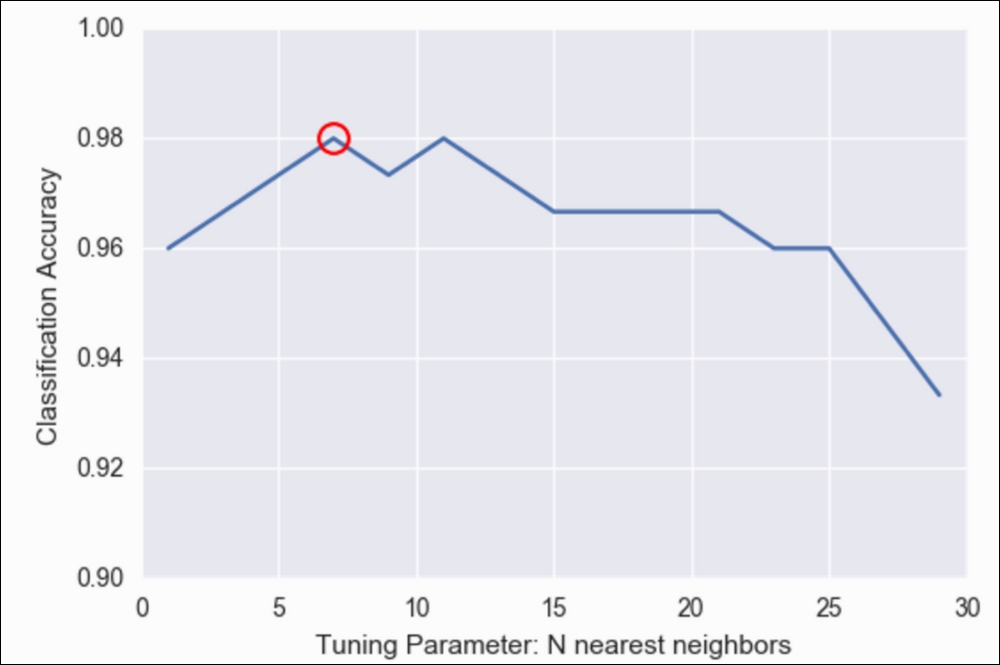
Classification Accuracy versus Tuning Parameters in N nearest neighbors
Note that the preceding graph is basically the same as the one we achieved previously with our for loop, but much easier!
We see that seven neighbors (circled in the preceding graph) seem to have the best accuracy. However, we can also, very easily, get our best parameters and our best model, as shown:
grid.best_params_
# {'n_neighbors': 7}

grid.best_score_
# 0.9799999999

grid.best_estimator_
# actually returns the unfit model with the best parameters
# KNeighborsClassifier(algorithm='auto', leaf_size=30, metric='minkowski', metric_params=None, n_jobs=1, n_neighbors=7, p=2, weights='uniform')
I'll take this one step further. Maybe you've noted that KNN has other parameters as well, such as algorithm, p, and weights. A quick look at the scikit-learn documentation reveals that we have some options for each of these, which are as follows:
pis an integer and represents the type of distance we wish to use. By default, we usep=2, which is our standard distance formula.weightsis, by default,uniform, but can also bedistance, which weighs points by their distance, meaning that close neighbors have a greater impact on the prediction.algorithmis how the model finds the nearest neighbors. We can tryball_tree,kd_tree, orbrute. The default is auto, which tries to use the best one automatically:knn = KNeighborsClassifier() k_range = range(1, 30) algorithm_options = ['kd_tree', 'ball_tree', 'auto', 'brute'] p_range = range(1, 8) weight_range = ['uniform', 'distance'] param_grid = dict(n_neighbors=k_range, weights=weight_range, algorithm=algorithm_options, p=p_range) # trying many more options grid = GridSearchCV(knn, param_grid, cv=5, scoring='accuracy') grid.fit(X, y)
The preceding code takes about a minute to run on my laptop because it is trying many, 1, 648, different combinations of parameters and cross-validating each one five times. All in all, to get the best answer, it is fitting 8,400 different KNN models:
grid.best_score_
0.98666666

grid.best_params_
{'algorithm': 'kd_tree', 'n_neighbors': 6, 'p': 3, 'weights': 'uniform'}
Grid searching is a simple (but inefficient) way of parameter tuning our models to get the best possible outcome. It should be noted that to get the best possible outcome, data scientists should use feature manipulation (both reduction and engineering) to obtain better results in practice as well. It should not merely be up to the model to achieve the best performance.
I think it is important once again to go over and compare the cross-validation error and the training error. This time, let's put them both on the same graph to compare how they both change as we vary the model complexity.
I will use the mammal dataset once more to show the cross-validation error and the training error (the error on predicting the training set). Recall that we are attempting to regress the body weight of a mammal to the brain weight of a mammal:
# This function uses a numpy polynomial fit function to
# calculate the RMSE of given X and y
def rmse(x, y, coefs):
    yfit = np.polyval(coefs, x)
    rmse = np.sqrt(np.mean((y - yfit) ** 2))
    return rmse

xtrain, xtest, ytrain, ytest = train_test_split(df['body'], df['brain'])

train_err = []
validation_err = []
degrees = range(1, 8)

for i, d in enumerate(degrees):
    p = np.polyfit(xtrain, ytrain, d)
  # built in numpy polynomial fit function

    train_err.append(rmse(xtrain, ytrain, p))
    validation_err.append(rmse(xtest, ytest, p))


fig, ax = plt.subplots()
# begin to make our graph

ax.plot(degrees, validation_err, lw=2, label = 'cross-validation error')
ax.plot(degrees, train_err, lw=2, label = 'training error')
# Our two curves, one for training error, the other for cross validation

ax.legend(loc=0)
ax.set_xlabel('degree of polynomial')
ax.set_ylabel('RMSE') 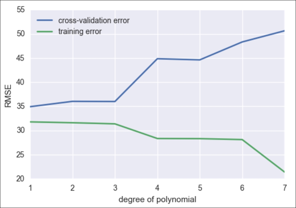
So, we see that as we increase our degree of fit, our training error goes down without a hitch, but we are now smart enough to know that as we increase the model complexity, our model is overfitting to our data and is merely regurgitating our data back to us, whereas our cross-validation error line is much more honest and begins to perform poorly after about degree 2 or 3.
Let's recap:
- Underfitting occurs when the cross-validation error and the training error are both high
- Overrfitting occurs when the cross-validation error is high, while the training error is low
- We have a good fit when the cross-validation error is low, and only slightly higher than the training error
Both underfitting (high bias) and overfitting (high variance) will result in poor generalization of the data.
Here are some tips if you face high bias or variance.
Try the following if your model tends to have a high bias:
- Try adding more features to the training and test sets
- Either add to the complexity of your model or try a more modern sophisticated model
Try the following if your model tends to have a high variance:
- Try to include more training samples, which reduces the effect of overfitting
In general, the bias/variance tradeoff is the struggle to minimize the bias and variance in our learning algorithms. Many newer learning algorithms, invented in the past few decades, were made with the intention of having the best of both worlds.