
Hypothesis tests are one of the most widely used tests in statistics. They come in many forms; however, all of them have the same basic purpose.
A hypothesis test is a statistical test that is used to ascertain whether we are allowed to assume that a certain condition is true for the entire population, given a data sample. Basically, a hypothesis test is a test for a certain hypothesis that we have about an entire population. The result of the test then tells us whether we should believe the hypothesis or reject it for an alternative one.
You can think of the hypothesis test's framework to determine whether the observed sample data deviates from what was to be expected from the population itself. Now, this sounds like a difficult task but, luckily, Python comes to the rescue and includes built-in libraries to conduct these tests easily.
A hypothesis test generally looks at two opposing hypotheses about a population. We call them the null hypothesis and the alternative hypothesis. The null hypothesis is the statement being tested and is the default correct answer; it is our starting point and our original hypothesis. The alternative hypothesis is the statement that opposes the null hypothesis. Our test will tell us which hypothesis we should trust and which we should reject.
Based on sample data from a population, a hypothesis test determines whether or not to reject the null hypothesis. We usually use a p-value (which is based on our significance level) to make this conclusion.
The following are some examples of questions you can answer with a hypothesis test:
- Does the mean break time of employees differ from 40 minutes?
- Is there a difference between people who interacted with website A and people who interacted with website B (A/B testing)?
- Does a sample of coffee beans vary significantly in taste from the entire population of beans?
There are multiple types of hypothesis tests out there, and among them are dozens of different procedures and metrics. Nonetheless, there are five basic steps that most hypothesis tests follow, which are as follows:
- Specify the hypotheses:
- Here, we formulate our two hypotheses: the null and the alternative.
- We usually use the notation of H0 to represent the null hypothesis and Ha to represent our alternative hypothesis.
- Determine the sample size for the test sample:
- This calculation depends on the chosen test. Usually, we have to determine a proper sample size in order to utilize theorems, such as the central limit theorem and assume the normality of data.
- Choose a significance level (usually called alpha or α):
- A significance level of 0.05 is common.
- Collect the data:
- Collect a sample of data to conduct the test.
- Decide whether to reject or fail to reject the null hypothesis:
- This step changes slightly based on the type of test being used. The final result will either yield a rejection of the null hypothesis in favor of the alternative or fail to reject the null hypothesis.
In this chapter, we will look at the following three types of hypothesis tests:
- One-sample t-tests
- Chi-square goodness of fit
- Chi-square test for association/independence
There are many more tests. However, these three are a great combination of distinct, simple, and powerful tests. One of the biggest things to consider when choosing which test we should implement is the type of data we are working with, specifically, are we dealing with continuous or categorical data? In order to truly see the effects of a hypothesis, I suggest we dive right into an example. First, let's look at the use of t-tests to deal with continuous data.
The one sample t-test is a statistical test used to determine whether a quantitative (numerical) data sample differs significantly from another dataset (the population or another sample). Suppose, in our previous employee break time example, we look, specifically, at the engineering department's break times, as shown:
long_breaks_in_engineering = stats.poisson.rvs(loc=10, mu=55, size=100)


short_breaks_in_engineering = stats.poisson.rvs(loc=10, mu=15, size=300)


engineering_breaks = np.concatenate((long_breaks_in_engineering, short_breaks_in_engineering))


print(breaks.mean())

# 39.99


print(engineering_breaks.mean())

# 34.825
Note that I took the same approach as making the original break times, but with the following two differences:
- I took a smaller sample from the Poisson distribution (to simulate that we took a sample of 400 people from the engineering department).
- Instead of using μ of 60 as before, I used 55 to simulate the fact that the engineering department's break behavior isn't exactly the same as the company's behavior as a whole.
It is easy to see that there seems to be a difference (of over 5 minutes) between the engineering department and the company as a whole. We usually don't have the entire population and the population parameters at our disposal, but I have them simulated in order for the example to work. So, even though we (the omniscient readers) can see a difference, we will assume that we know nothing of these population parameters and, instead, rely on a statistical test in order to ascertain these differences.
Our objective here is to ascertain whether there is a difference between the overall population's (company employees) break times and the break times of employees in the engineering department.
Let's now conduct a t-test at a 95% confidence level in order to find a difference (or not!). Technically speaking, this test will tell us if the sample comes from the same distribution as the population.
Before diving into the five steps, we must first acknowledge that t-tests must satisfy the following two conditions to work properly:
- The population distribution should be normal, or the sample should be large (n ≥ 30)
- In order to make the assumption that the sample is independently, randomly sampled, it is sufficient to enforce that the population size should be at least 10 times larger than the sample size (10n < N)
Note that our test requires that either the underlying data be normal (which we know is not true for us), or that the sample size is at least 30 points large. For the t-test, this condition is sufficient to assume normality. This test also requires independence, which is satisfied by taking a sufficiently small sample. Sounds weird, right? The basic idea is that our sample must be large enough to assume normality (through conclusions similar to the central limit theorem) but small enough as to be independent of the population.
Now, let's follow our five steps:
- Specify the hypotheses.
We will let H 0 = the engineering department take breaks of the same duration as the company as a whole
If we let this be the company average, we may write the following:
Note how this is our null, or default, hypothesis. It is what we would assume, given no data. What we would like to show is the alternative hypothesis.
Now that we actually have some options for our alternative, we could either say that the engineering mean (let's call it that) is lower than the company average, higher than the company average, or just flat out different (higher or lower) than the company average:
- If we wish to answer the question, "is the sample mean different from the company average?," then this is called a two-tailed test and our alternative hypothesis would be as follows:

- If we want to find out whether the sample mean is lower than the company average or if the sample mean is higher than the company average, then we are dealing with a one-tailed test and our alternative hypothesis would be one of the following hypotheses:
Ha:(engineering takes longer breaks)
Ha:(engineering takes shorter breaks)
The difference between one and two tails is the difference of dividing a number later on by two or not. The process remains completely unchanged for both. For this example, let's choose the two-tailed test. So, we are testing for whether or not this sample of the engineering department's average break times is different from the company average.
Note
Our test will end in one of two possible conclusions: we will either reject the null hypothesis, which means that the engineering department's break times are different from the company average, or we will fail to reject the null hypothesis, which means that there wasn't enough evidence in the sample to support rejecting the null.
- If we wish to answer the question, "is the sample mean different from the company average?," then this is called a two-tailed test and our alternative hypothesis would be as follows:
- Determine the sample size for the test sample.
As mentioned earlier, most tests (including this one) make the assumption that either the underlying data is normal or that our sample is in the right range:
- The sample is at least 30 points (it is 400)
- The sample is less than 10% of the population (which would be 900 people)
- Choose a significance level (usually called alpha or α). We will choose a 95% significance level, which means that our alpha would actually be 1 - .95 = .05
- Collect the data. This is generated through the two Poisson distributions.
- Decide whether to reject or fail to reject the null hypothesis. As mentioned before, this step varies based on the test used. For a one-sample t-test, we must calculate two numbers: the test statistic and our p-value. Luckily, we can do this in one line in Python.
A test statistic is a value that is derived from sample data during a type of hypothesis test. They are used to determine whether or not to reject the null hypothesis.
The test statistic is used to compare the observed data with what is expected under the null hypothesis. The test statistic is used in conjunction with the p-value.
The p-value is the probability that the observed data occurred this way by chance.
When the data is showing very strong evidence against the null hypothesis, the test statistic becomes large (either positive or negative) and the p-value usually becomes very small, which means that our test is showing powerful results and what is happening is, probably, not happening by chance.
In the case of a t-test, a t value is our test statistic, as shown:
t_statistic, p_value = stats.ttest_1samp(a= engineering_breaks,
 popmean= breaks.mean())
We input the engineering_breaks variable (which holds 400 break times) and the population mean (popmean), and we obtain the following numbers:
t_statistic == -5.742

p_value == .00000018
The test result shows that the t value is -5.742. This is a standardized metric that reveals the deviation of the sample mean from the null hypothesis. The p-value is what gives us our final answer. Our p-value is telling us how often our result would appear by chance. So, for example, if our p-value was .06, then that would mean we should expect to observe this data by chance about 6% of the time. This means that about 6% of samples would yield results like this.
We are interested in how our p-value compares to our significance level:
- If the p-value is less than the significance level, then we can reject the null hypothesis
- If the p-value is greater than the significance level, then we failed to reject the null hypothesis
Our p-value is way lower than .05 (our chosen significance level), which means that we may reject our null hypothesis in favor of the alternative. This means that the engineering department seems to take different break lengths than the company as a whole!
Note
The use of p-values is controversial. Many journals have actually banned the use of p-values in tests for significance. This is because of the nature of the value. Suppose our p-value came out to .04. It means that 4% of the time, our data just randomly happened to appear this way and is not significant in any way. 4% is not that small of a percentage! For this reason, many people are switching to different statistical tests. However, that does not mean that p-values are useless. It merely means that we must be careful and aware of what the number is telling us.
There are many other types of t-tests, including one-tailed tests (mentioned before) and paired tests as well as two sample t-tests (both not mentioned yet). These procedures can be readily found in statistics literature; however, we should look at something very important—what happens when we get it wrong.
We've mentioned both the type I and type II errors in Chapter 5, Impossible or Improbable – A Gentle Introduction to Probability, about probability in the examples of a binary classifier, but they also apply to hypothesis tests.
A type I error occurs if we reject the null hypothesis when it is actually true. This is also known as a false positive. The type I error rate is equal to the significance level α, which means that if we set a higher confidence level, for example, a significance level of 99%, our α is .01, and therefore our false positive rate is 1%.
A type II error occurs if we fail to reject the null hypothesis when it is actually false. This is also known as a false negative. The higher we set our confidence level, the more likely we are to actually see a type II error.
T-tests (among other tests) are hypothesis tests that work to compare and contrast quantitative variables and underlying population distributions. In this section, we will explore two new tests, both of which serve to explore qualitative data. They are both a form of test called chi-square tests. These two tests will perform the following two tasks for us:
The one-sample t-test was used to check whether a sample means differed from the population mean. The chi-square goodness of fit test is very similar to the one sample t-test in that it tests whether the distribution of the sample data matches an expected distribution, while the big difference is that it is testing for categorical variables.
For example, a chi-square goodness of fit test would be used to see whether the race demographics of your company match that of the entire city of the U.S. population. It can also be used to see if users of your website show similar characteristics to average internet users.
As we are working with categorical data, we have to be careful because categories such as "male," "female," or "other" don't have any mathematical meaning. Therefore, we must consider counts of the variables rather than the actual variables themselves.
In general, we use the chi-square goodness of fit test in the following cases:
- We want to analyze one categorical variable from one population
- We want to determine whether a variable fits a specified or expected distribution
In a chi-square test, we compare what is observed to what we expect.
There are two usual assumptions of this test, as follows:
- All the expected counts are at least five
- Individual observations are independent and the population should be at least 10 times as large as the sample (10n < N)
The second assumption should look familiar to the t-test; however, the first assumption should look foreign. Expected counts are something we haven't talked about yet but are about to!
When formulating our null and alternative hypotheses for this test, we consider a default distribution of categorical variables. For example, if we have a die and we are testing whether or not the outcomes are coming from a fair die, our hypothesis might look as follows:

Our alternative hypothesis is quite simple, as shown:
H a : The specified distribution of the categorical variable is not correct. At least one of the pi values is not correct.
In the t-test, we used our test statistic (the t-value) to find our p-value. In a chi-square test, our test statistic is, well, a chi-square:

A critical value is when we use χ 2 as well as our degrees of freedom and our significance level, and then reject the null hypothesis if the p-value is below our significance level (the same as before).
Let's look at an example to understand this further.
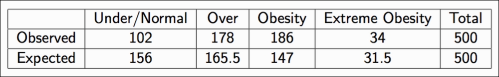
The CDC categorizes adult BMIs into four classes: Under/Normal, Over, Obesity, and Extreme Obesity. A 2009 survey showed the distribution for adults in the US to be 31.2%, 33.1%, 29.4%, and 6.3% respectively. A total of 500 adults were randomly sampled and their BMI categories were recorded. Is there evidence to suggest that BMI trends have changed since 2009? Let's test at the 0.05 significance level:

First, let's calculate our expected values. In a sample of 500, we expect 156 to be Under/Normal (that's 31.2% of 500), and we fill in the remaining boxes in the same way:
First, check the conditions that are as follows:
- All of the expected counts are greater than five
- Each observation is independent and our population is very large (much more than 10 times of 500 people)
Next, carry out a goodness of fit test. We will set our null and alternative hypotheses:
- H0: The 2009 BMI distribution is still correct.
- Ha: The 2009 BMI distribution is no longer correct (at least one of the proportions is different now). We can calculate our test statistic by hand:

Alternatively, we can use our handy-dandy Python skills, as shown:
observed = [102, 178, 186, 34]

expected = [156, 165.5, 147, 31.5]


chi_squared, p_value = stats.chisquare(f_obs= observed, f_exp= expected)


chi_squared, p_value

#(30.1817679275599, 1.26374310311106e-06)
Our p-value is lower than .05; therefore, we may reject the null hypothesis in favor of the fact that the BMI trends today are different from what they were in 2009.
Independence as a concept in probability is when knowing the value of one variable tells you nothing about the value of another. For example, we might expect that the country and the month you were born in are independent. However, knowing which type of phone you use might indicate your creativity levels. Those variables might not be independent.
The chi-square test for association/independence helps us ascertain whether two categorical variables are independent of one another. The test for independence is commonly used to determine whether variables like education levels or tax brackets vary based on demographic factors, such as gender, race, and religion. Let's look back at an example posed in the preceding chapter, the A/B split test.
Recall that we ran a test and exposed half of our users to a certain landing page (Website A), exposed the other half to a different landing page (Website B), and then measured the sign-up rates for both sites. We obtained the following results:
|
Did not sign up |
Signed up | |
|
Website A |
134 |
54 |
|
Website B |
110 |
48 |
Results of our A/B test
We calculated website conversions but what we really want to know is whether there is a difference between the two variables: which website was the user exposed to? and did the user sign up? For this, we will use our chi-square test.
There are the following two assumptions of this test:
- All expected counts are at least five
- Individual observations are independent and the population should be at least 10 times as large as the sample (10n < N)
Note that they are exactly the same as the last chi-square test.
Let's set up our hypotheses:
- H0: There is no association between two categorical variables in the population of interest
- H0: Two categorical variables are independent in the population of interest
- Ha: There is an association between two categorical variables in the population of interest
- Ha: Two categorical variables are not independent in the population of interest
You might notice that we are missing something important here. Where are the expected counts? Earlier, we had a prior distribution to compare our observed results to but now we do not. For this reason, we will have to create some. We can use the following formula to calculate the expected values for each value. In each cell of the table, we can use the following:

Here, r is the number of rows and c is the number of columns. Of course, as before, when we calculate our p-value, we will reject the null if that p-value is less than the significance level. Let's use some built-in Python methods, as shown, in order to quickly get our results:
observed = np.array([[134, 54],[110, 48]])

# built a 2x2 matrix as seen in the table above


chi_squared, p_value, degrees_of_freedom, matrix = stats.chi2_contingency(observed= observed)


chi_squared, p_value

# (0.04762692369491045, 0.82724528704422262)
We can see that our p-value is quite large; therefore, we fail to reject our null hypothesis and we cannot say for sure that seeing a particular website has any effect on a whether or not a user signs up. There is no association between these variables.