
When you ask a data scientist, "what type of data is this?", they will usually assume that you are asking them whether or not it is mostly quantitative or qualitative. It is likely the most common way of describing the specific characteristics of a dataset.
For the most part, when talking about quantitative data, you are usually (not always) talking about a structured dataset with a strict row/column structure (because we don't assume unstructured data even has any characteristics). All the more reason why the pre-processing step is so important.
These two data types can be defined as follows:
- Quantitative data: This data can be described using numbers, and basic mathematical procedures, including addition, are possible on the set.
- Qualitative data: This data cannot be described using numbers and basic mathematics. This data is generally thought of as being described using natural categories and language.
Say that we were processing observations of coffee shops in a major city using the following five descriptors (characteristics):
Data: Coffee Shop
- Name of coffee shop
- Revenue (in thousands of dollars)
- Zip code
- Average monthly customers
- Country of coffee origin
Each of these characteristics can be classified as either quantitative or qualitative, and that simple distinction can change everything. Let's take a look at each one:
- Name of a coffee shop: Qualitative
The name of a coffee shop is not expressed as a number and we cannot perform mathematical operations on the name of the shop.
- Revenue: Quantitative
How much money a coffee shop brings in can definitely be described using a number. Also, we can do basic operations, such as adding up the revenue for 12 months to get a year's worth of revenue.
- Zip code: Qualitative
This one is tricky. A zip code is always represented using numbers, but what makes it qualitative is that it does not fit the second part of the definition of quantitative—we cannot perform basic mathematical operations on a zip code. If we add together two zip codes, it is a nonsensical measurement. We don't necessarily get a new zip code and we definitely don't get "double the zip code."
- Average monthly customers: Quantitative
Again, describing this factor using numbers and addition makes sense. Add up all of your monthly customers and you get your yearly customers.
- Country of coffee origin: Qualitative
We will assume this is a very small coffee shop with coffee from a single origin. This country is described using a name (Ethiopian, Colombian), and not numbers.
A couple of important things to note:
- Even though a zip code is being described using numbers, it is not quantitative. This is because you can't talk about the sum of all zip codes or an average zip code. These are nonsensical descriptions.
- Pretty much whenever a word is used to describe a characteristic, it is a qualitative factor.
If you are having trouble identifying which is which, basically, when trying to decide whether or not the data is qualitative or quantitative, ask yourself a few basic questions about the data characteristics:
- Can you describe it using numbers?
- No? It is qualitative
- Yes? Move on to the next question
- Does it still make sense after you add them together?
- No? They are qualitative
- Yes? You probably have quantitative data
This method will help you to classify most, if not all, data into one of these two categories.
The difference between these two categories defines the types of questions you may ask about each column. For a quantitative column, you may ask questions such as the following:
- What is the average value?
- Does this quantity increase or decrease over time (if time is a factor)?
- Is there a threshold where if this number became too high or too low, it would signal trouble for the company?
For a qualitative column, none of the preceding questions can be answered. However, the following questions only apply to qualitative values:
The World Health Organization (WHO) released a dataset describing the average drinking habits of people in countries across the world. We will use Python and the data exploration tool, pandas, in order to gain a better look:
import pandas as pd

# read in the CSV file from a URL
drinks = pd.read_csv('https://raw.githubusercontent.com/sinanuozdemir/principles_of_data_science/master/data/chapter_2/drinks.csv')

# examine the data's first five rows
drinks.head()           # print the first 5 rows
These three lines have done the following:
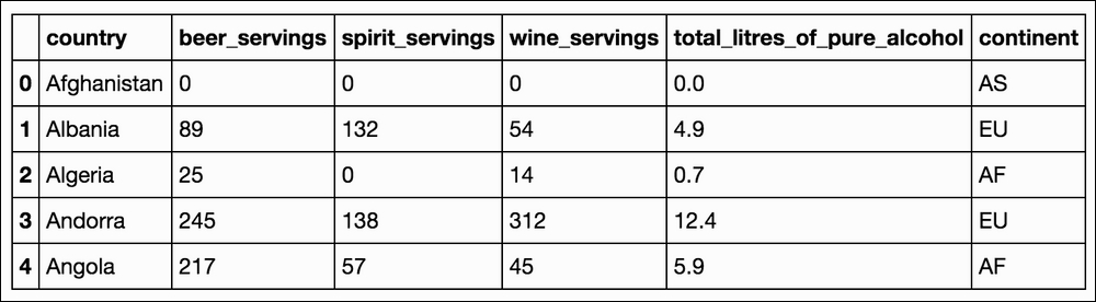
The preceding table lists the first five rows of data from the drink.csv file. We have six different columns that we are working within this example:
country: Qualitativebeer_servings: Quantitativespirit_servings: Quantitativewine_servings: Quantitativetotal_litres_of_pure_alcohol: Quantitativecontinent: Qualitative
Let's look at the qualitative column continent. We can use Pandas in order to get some basic summary statistics about this non-numerical characteristic. The describe() method is being used here, which first identifies whether the column is likely to be quantitative or qualitative, and then gives basic information about the column as a whole. This is done as follows:
drinks['continent'].describe()

>> count     170
>> unique      5
>> top        AF
>> freq       53
It reveals that the WHO has gathered data about five unique continents, the most frequent being AF (Africa), which occurred 53 times in the 193 observations.
If we take a look at one of the quantitative columns and call the same method, we can see the difference in output, as shown:
drinks['beer_servings'].describe()
The output is as follows:
count    193.000000
mean     106.160622
std      101.143103
min        0.000000
25%       20.000000
50%       76.000000
75%      188.000000
max      376.000000
Now, we can look at the mean (average) beer serving per person per country (106.2 servings), as well as the lowest beer serving, zero, and the highest beer serving recorded, 376 (that's more than a beer a day).
Quantitative data can be broken down one step further into discrete and continuous quantities.
These can be defined as follows:
- Discrete data: This describes data that is counted. It can only take on certain values.Examples of discrete quantitative data include a dice roll, because it can only take on six values, and the number of customers in a coffee shop, because you can't have a real range of people.
- Continuous data: This describes data that is measured. It exists on an infinite range of values.A good example of continuous data would be a person's weight, because it can be 150 pounds or 197.66 pounds (note the decimals). The height of a person or building is a continuous number because an infinite scale of decimals is possible. Other examples of continuous data would be time and temperature.