11
FIGHTING A SLOW NETWORK

As a network administrator, much of your time will be spent fixing computers and services that are running slower than they should be. But just because someone says that the network is running slowly doesn’t mean that the network is to blame.

Before you begin to tackle a slow network, you first need to determine whether the network is in fact running slowly. You’ll learn how to do that in this chapter.

We’ll begin by discussing the error-recovery and flow-control features of TCP. Then we’ll explore how to detect the source of slowness on a network. Finally, we’ll look at ways of baselining networks and the devices and services that run on them. Once you have completed this chapter, you should be much better equipped to identify, diagnose, and troubleshoot slow networks.

TCP Error-Recovery Features

TCP’s error-recovery features are our best tools for locating, diagnosing, and eventually repairing high latency on a network. In terms of computer networking, latency is a measure of delay between a packet’s transmission and its receipt.

Latency can be measured as one-way (from a single source to a destination) or as round-trip (from a source to a destination and back to the original source). When communication between devices is fast, and the amount of time it takes a packet to get from one point to another is low, the communication is said to have low latency. Conversely, when packets take a significant amount of time to travel between a source and destination, the communication is said to have high latency. High latency is the number one enemy of all network administrators who value their sanity (and their jobs).

In Chapter 8, we discussed how TCP uses sequence and acknowledgment numbers to ensure the reliable delivery of packets. In this chapter, we’ll look at sequence and acknowledgment numbers again to see how TCP responds when high latency causes these numbers to be received out of sequence (or not received at all).

TCP Retransmissions

The ability of a host to retransmit packets is one of TCP’s most fundamental error-recovery features. It is designed to combat packet loss.

There are many possible causes of packet loss, including malfunctioning applications, routers under a heavy traffic load, or temporary service outages. Things move fast at the packet level, and often the packet loss is temporary, so it’s crucial for TCP to be able to detect and recover from packet loss.

The primary mechanism for determining whether the retransmission of a packet is necessary is the retransmission timer. This timer is responsible for maintaining a value called the retransmission timeout (RTO). Whenever a packet is transmitted using TCP, the retransmission timer starts. This timer stops when an ACK for that packet is received. The time between the packet transmission and receipt of the ACK packet is called the round-trip time (RTT). Several of these times are averaged, and that average is used to determine the final RTO value.

Until an RTO value is determined, the transmitting operating system relies on its default configured RTT setting, which is issued for the initial communication between hosts. This is then adjusted based on the RTT of received packets to determine the RTO value.

Once the RTO value has been determined, the retransmission timer is used on every transmitted packet to determine whether packet loss has occurred. Figure 11-1 illustrates the TCP retransmission process.

Figure 11-1: Conceptual view of the TCP retransmission process

When a packet is sent, but the recipient has not sent back a TCP ACK packet, the transmitting host assumes that the original packet was lost and retransmits the original packet. When the retransmission is sent, the RTO value is doubled; if no ACK packet is received before that value is reached, another retransmission will occur. If this retransmission also does not receive an ACK response, the RTO value is doubled again. This process will continue, with the RTO value being doubled for each retransmission, until an ACK packet is received or until the sender reaches the maximum number of retransmission attempts it is configured to send. More details about this process are described in RFC6298.

The maximum number of retransmission attempts depends on the value configured in the transmitting operating system. By default, Windows hosts make a maximum of five retransmission attempts. Most Linux hosts default to a maximum of 15 attempts. This option is configurable in either operating system.

For an example of TCP retransmission, open the file tcp_retransmissions.pcapng, which contains six packets. The first packet is shown in Figure 11-2.

Figure 11-2: A simple TCP packet containing data

This packet is a TCP PSH/ACK packet ➋ containing 648 bytes of data ➌ that are sent from 10.3.30.1 to 10.3.71.7 ➊. This is a typical data packet.

Under normal circumstances, you would expect to see a TCP ACK packet in response fairly soon after the first packet is sent. In this case, however, the next packet is a retransmission. You can tell this by looking at the packet in the Packet List pane. The Info column will clearly say [TCP Retransmission], and the packet will appear with red text on a black background. Figure 11-3 shows examples of retransmissions listed in the Packet List pane.

Figure 11-3: Retransmissions in the Packet List pane

You can also determine whether a packet is a retransmission by examining it in the Packet Details pane, as shown in Figure 11-4.

In the Packet Details pane, notice that the retransmission packet has some additional information included under the SEQ/ACK analysis heading ➊. This useful information is provided by Wireshark and is not contained in the packet itself. The SEQ/ACK analysis tells us that this is indeed a retransmission ➋, that the RTO value is 0.206 seconds ➌, and that the RTO is based on the delta time from packet 1 ➍.

Figure 11-4: An individual retransmission packet

Note that this packet is the same as the original packet (other than the IP identification and Checksum fields). To verify this, compare the Packet Bytes pane of this retransmitted packet with the original one.

Examination of the remaining packets should yield similar results, with the only differences between the packets found in the IP identification and Checksum fields and in the RTO value. To visualize the time lapse between each packet, look at the Time column in the Packet List pane, as shown in Figure 11-5. Here, you see exponential growth in time as the RTO value is doubled after each retransmission.

The TCP retransmission feature is used by the transmitting device to detect and recover from packet loss. Next, we’ll examine TCP duplicate acknowledgments, a feature that the data recipient uses to detect and recover from packet loss.

Figure 11-5: The Time column shows the increase in RTO value.

TCP Duplicate Acknowledgments and Fast Retransmissions

A duplicate ACK is a TCP packet sent from a recipient when that recipient receives packets that are out of order. TCP uses the sequence and acknowledgment number fields within its header to reliably ensure that data is received and reassembled in the same order in which it was sent.

When a new TCP connection is established, one of the most important pieces of information exchanged during the handshake process is an initial sequence number (ISN). Once the ISN is set for each side of the connection, each subsequently transmitted packet increments the sequence number by the size of its data payload.

Consider a host that has an ISN of 5000 and sends a 500-byte packet to a recipient. Once this packet has been received, the recipient host will respond with a TCP ACK packet with an acknowledgment number of 5500, based on the following formula:

Sequence Number In + Bytes of Data Received = Acknowledgment Number Out

As a result of this calculation, the acknowledgment number returned to the transmitting host is the next sequence number that the recipient expects to receive. An example of this can be seen in Figure 11-6.

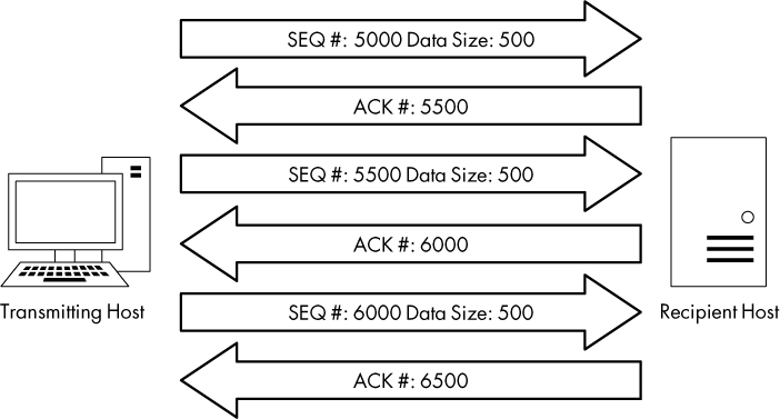
Figure 11-6: TCP sequence and acknowledgment numbers

The detection of packet loss by the data recipient is made possible through the sequence numbers. As the recipient tracks the sequence numbers it is receiving, it can determine when it receives sequence numbers that are out of order.

When the recipient receives an unexpected sequence number, it assumes that a packet has been lost in transit. To reassemble data properly, the recipient must have the missing packet, so it resends the ACK packet that contains the lost packet’s expected sequence number in order to elicit a retransmission of that packet from the transmitting host.

When the transmitting host receives three duplicate ACKs from the recipient, it assumes that the packet was indeed lost in transit and immediately sends a fast retransmission. Once a fast retransmission is triggered, all other packets being transmitted are queued until the fast retransmission packet is sent. This process is depicted in Figure 11-7.

Figure 11-7: Duplicate ACKs from the recipient result in a fast retransmission.

You’ll find an example of duplicate ACKs and fast retransmissions in the file tcp_dupack.pcapng. The first packet in this capture is shown in Figure 11-8.

Figure 11-8: The ACK showing the next expected sequence number

This packet, a TCP ACK sent from the data recipient (172.31.136.85) to the transmitter (195.81.202.68) ➊, has an acknowledgment of the data sent in the previous packet that is not included in this capture file.

The acknowledgment number in this packet is 1310973186 ➋. This should match the sequence number in the next packet received, as shown in Figure 11-9.

Figure 11-9: The sequence number of this packet is not what was expected.

Unfortunately for us and our recipient, the sequence number of the next packet is 1310984130 ➊, which is not what we expect. This out-of-order packet indicates that the expected packet was somehow lost in transit. The recipient host notices that this packet is out of sequence and sends a duplicate ACK in the third packet of this capture, as shown in Figure 11-10.

You can determine that this is a duplicate ACK packet by examining either of the following:

•     The Info column in the Packet Details pane. The packet should appear as red text on a black background.

•     The Packet Details pane under the SEQ/ACK analysis heading (Figure 11-10). If you expand this heading, you’ll find that the packet is listed as a duplicate ACK of packet 1 ➊.

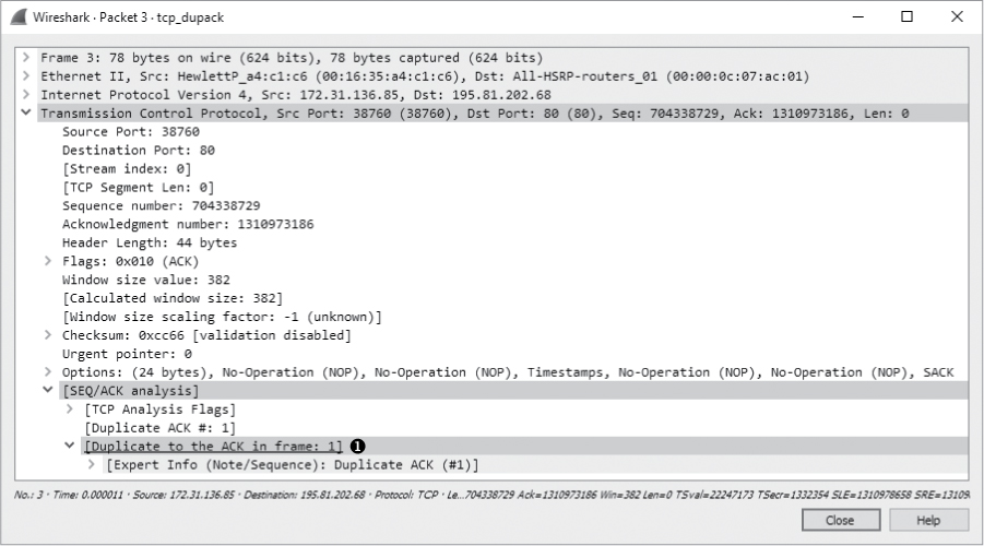
Figure 11-10: The first duplicate ACK packet

The next several packets continue this process, as shown in Figure 11-11.

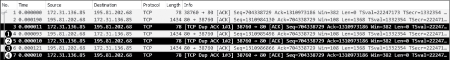
Figure 11-11: Additional duplicate ACKs are generated due to out-of-order packets.

The fourth packet in the capture file is another chunk of data sent from the transmitting host with the wrong sequence number ➊. As a result, the recipient host sends its second duplicate ACK ➋. One more packet with the wrong sequence number is received by the recipient ➌. That prompts the transmission of the third and final duplicate ACK ➍.

As soon as the transmitting host receives the third duplicate ACK from the recipient, it is forced to halt all packet transmission and resend the lost packet. Figure 11-12 shows the fast retransmission of the lost packet.

The retransmission packet can once again be found through the Info column in the Packet List pane. As with previous examples, the packet is clearly labeled with red text on a black background. The SEQ/ACK analysis section of this packet (Figure 11-12) tells us that this is suspected to be a fast retransmission ➊. (Again, the information that labels this packet as a fast retransmission is not a value set in the packet itself but rather a feature of Wireshark.) The final packet in the capture is an ACK packet acknowledging receipt of the fast retransmission.

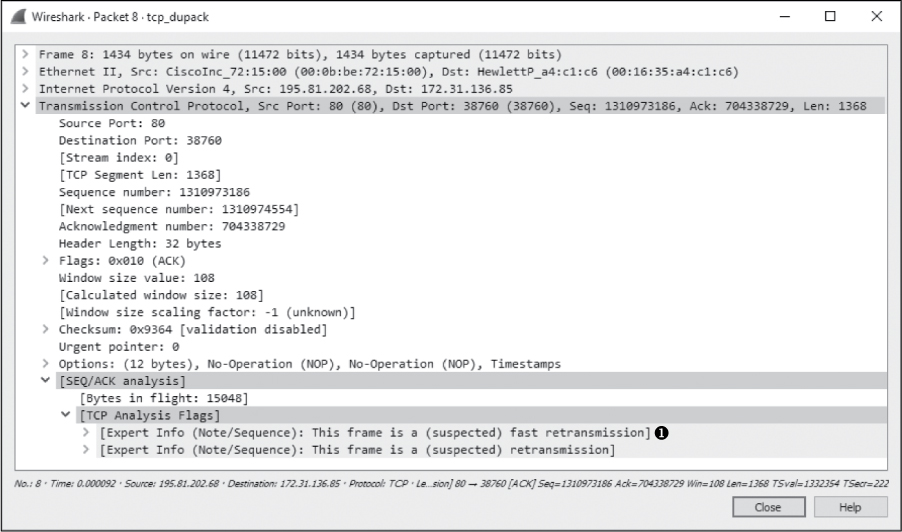
Figure 11-12: Three duplicate ACKs cause this fast retransmission of the lost packet.

TCP Flow Control

Retransmissions and duplicate ACKs are reactive TCP functions designed to recover from packet loss. TCP would be a poor protocol indeed if it didn’t include some form of proactive method for preventing packet loss.

TCP implements a sliding-window mechanism to detect when packet loss may occur and adjust the rate of data transmission to prevent it. The sliding-window mechanism leverages the data recipient’s receive window to control the flow of data.

The receive window is a value specified by the data recipient and stored in the TCP header (in bytes) that tells the transmitting device how much data the recipient is willing to store in its TCP buffer space. This buffer space is where data is stored temporarily until it can be passed up the stack to the application-layer protocol waiting to process it. As a result, the transmitting host can send only the amount of data specified in the Window size value field at one time. For the transmitter to send more data, the recipient must send an acknowledgment that the previous data was received. It also must clear TCP buffer space by processing the data that is occupying that position. Figure 11-13 illustrates how the receive window works.

Figure 11-13: The receive window keeps the data recipient from getting overwhelmed.

In Figure 11-13, the client is sending data to a server that has communicated a receive window size of 5,000 bytes. The client sends 2,500 bytes, reducing the server’s buffer space to 2,500 bytes, and then sends another 2,000 bytes, further reducing the buffer to 500 bytes. The server sends an acknowledgment of this data, and after it processes the data in its buffer, it again has an empty buffer available. This process repeats, with the client sending 3,000 bytes and another 1,000 bytes, reducing the server’s buffer to 1,000 bytes. The client once more acknowledges this data and processes the contents of its buffer.

Adjusting the Window Size

This process of adjusting the window size is fairly clear-cut, but it isn’t always perfect. Whenever data is received by the TCP stack, an acknowledgment is generated and sent in reply, but the data placed in the recipient’s buffer is not always processed immediately.

When a busy server is processing packets from multiple clients, it could quite possibly be slow in clearing its buffer and thus be unable to make room for new data. Without a means of flow control, a full buffer could lead to lost packets and data corruption. Fortunately, when a server becomes too busy to process data at the rate its receive window is advertising, it can adjust the size of the window. It does this by decreasing the window size value in the TCP header of the ACK packet it is sending back to the hosts that are sending it data. Figure 11-14 shows an example of this.

Figure 11-14: The window size can be adjusted when the server becomes busy.

In Figure 11-14, the server starts with an advertised window size of 5,000 bytes. The client sends 2,000 bytes, followed by another 2,000 bytes, leaving only 1,000 bytes of buffer space available. The server realizes that its buffer is filling up quickly and knows that if data transfer keeps up at this rate, packets will soon be lost. To avoid such a mishap, the server sends an acknowledgment to the client with an updated window size of 1,000 bytes. The client responds by sending less data, and now the rate at which the server can process its buffer contents allows data to flow in a constant manner.

The resizing process works both ways. When the server can process data at a faster rate, it can send an ACK packet with a larger window size.

Halting Data Flow with a Zero Window Notification

Due to a lack of memory, a lack of processing capability, or another problem, a server may no longer process data sent from a client. Such a stoppage could result in dropped packets and a halting of the communication process, but the receive window can minimize negative effects.

When this situation arises, a server can send a packet that contains a window size of zero. When the client receives this packet, it will halt any data transmission but will sometimes keep the connection to the server open with the transmission of keep-alive packets. Keep-alive packets can be sent by the client at regular intervals to check the status of the server’s receive window. Once the server can begin processing data again, it will respond with a nonzero window size, and communication will resume. Figure 11-15 illustrates an example of zero window notification.

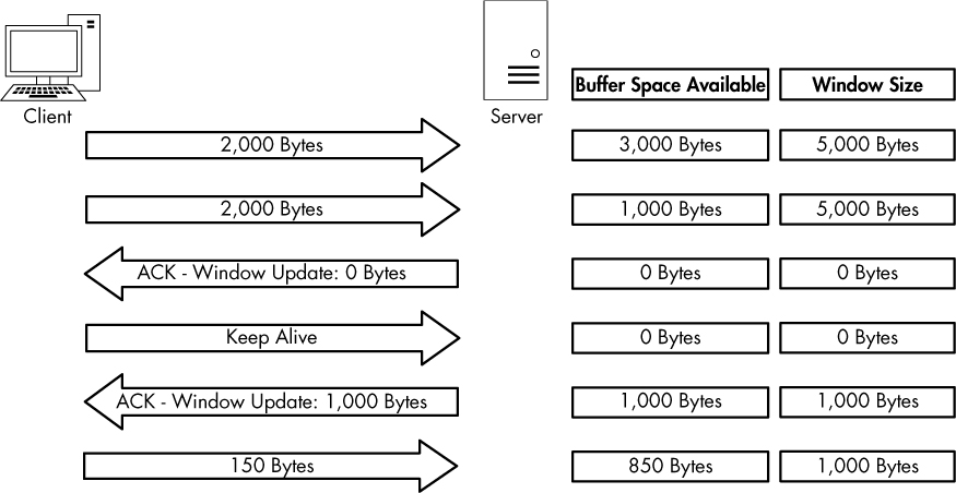
Figure 11-15: Data transfer stops when the window size is set to 0 bytes.

In Figure 11-15, the server begins receiving data with a 5,000-byte window size. After receiving a total of 4,000 bytes of data from the client, the server begins experiencing a very heavy processor load, and it can no longer process any data from the client. The server then sends a packet with the Window size value field set to 0. The client halts transmission of data and sends a keep-alive packet. After receiving the keep-alive packet, the server responds with a packet notifying the client that it can now receive data and that its window size is 1,000 bytes. The client resumes sending data but at a slower rate than before.

The TCP Sliding Window in Practice

Having covered the theory behind the TCP sliding window, we will now examine it in the capture file tcp_zerowindowrecovery.pcapng.

In this file, we begin with several TCP ACK packets traveling from 192.168.0.20 to 192.168.0.30. The main value of interest to us is the Window size value field, which can be seen in both the Info column of the Packet List pane and in the TCP header in the Packet Details pane. You can see immediately that this field’s value decreases over the course of the first three packets, as shown in Figure 11-16.

Figure 11-16: The window size of these packets is decreasing.

The window size value goes from 8,760 bytes in the first packet to 5,840 bytes in the second packet and then 2,920 bytes in the third packet ➋. This lowering of the window size value is a classic indicator of increased latency from the host. Notice in the Time column that this happens very quickly ➊. When the window size is lowered this fast, it’s common for the window size to drop to zero, which is exactly what happens in the fourth packet, as shown in Figure 11-17.

Figure 11-17: This zero window packet says that the host cannot accept any more data.

The fourth packet is also being sent from 192.168.0.20 to 192.168.0.30, but its purpose is to tell 192.168.0.30 that it can no longer receive any data. The 0 value is seen in the TCP header ➊. Wireshark also tells us that this is a zero window packet in the Info column of the Packet List pane and under the SEQ/ACK analysis section of the TCP header ➋.

Once this zero window packet is sent, the device at 192.168.0.30 will not send any more data until it receives a window update from 192.168.0.20 notifying it that the window size has increased. Luckily for us, the issue causing the zero window condition in this capture file was only temporary. So, a window update is sent in the next packet, shown in Figure 11-18.

In this case, the window size is increased to a very healthy 64,240 bytes ➊. Wireshark once again lets us know that this is a window update under the SEQ/ACK analysis heading.

Once the update packet is received, the host at 192.168.0.30 can begin sending data again, as it does in packets 6 and 7. This entire period of halted data transmission takes place very quickly. Had it lasted only slightly longer, it could have caused a potential hiccup on the network, resulting in a slower or failed data transfer.

Figure 11-18: A TCP window update packet lets the other host know it can begin transmitting again.

For one last look at the sliding window, examine tcp_zerowindowdead.pcapng. The first packet in this capture is normal HTTP traffic being sent from 195.81.202.68 to 172.31.136.85. The packet is immediately followed with a zero window packet sent back from 172.31.136.85, as shown in Figure 11-19.

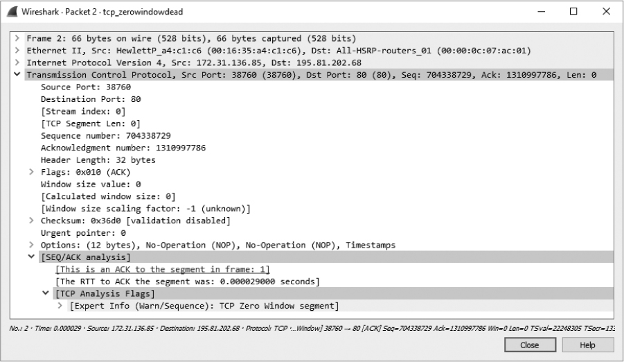
Figure 11-19: A zero window packet halts data transfer.

This looks very similar to the zero window packet shown in Figure 11-17, but the result is much different. Rather than seeing a window update from the 172.31.136.85 host and the resumption of communication, we see a keep-alive packet, as shown in Figure 11-20.

Figure 11-20: This keep-alive packet ensures the zero window host is still alive.

This packet is marked as a keep-alive by Wireshark under the SEQ/ACK analysis section of the TCP header in the Packet Details pane ➊. The Time column tells us that this packet was sent 3.4 seconds after the last received packet. This process continues several more times, with one host sending a zero window packet and the other sending a keep-alive packet, as shown in Figure 11-21.

Figure 11-21: The host and client continue to send zero window and keep-alive packets, respectively.

These keep-alive packets occur at intervals of 3.4, 6.8, and 13.5 seconds ➊. This process can go on for quite a long time, depending on the operating systems of the communicating devices. As you can see by adding up the values in the Time column, the connection is halted for nearly 25 seconds. Imagine attempting to authenticate with a domain controller or download a file from the internet while experiencing a 25-second delay—unacceptable!

Learning from TCP Error-Control and Flow-Control Packets

Let’s put retransmission, duplicate ACKs, and the sliding-window mechanism into some context. Here are a few notes to keep in mind when troubleshooting latency issues.

Retransmission Packets

Retransmissions occur because the client has detected that the server is not receiving the data it’s sending. Therefore, depending on which side of the communication you are analyzing, you may never see retransmissions. If you are capturing data from the server, and it is truly not receiving the packets being sent and retransmitted from the client, you may be in the dark because you won’t see the retransmission packets. If you suspect that you are the victim of packet loss on the server side, consider attempting to capture traffic from the client (if possible) so that you can see whether retransmission packets are present.

Duplicate ACK Packets

I tend to think of a duplicate ACK as the pseudo-opposite of a retransmission, because it is sent when the server detects that a packet from the client it is communicating with was lost in transit. In most cases, you can see duplicate ACKs when capturing traffic on both sides of the communication. Remember that duplicate ACKs are triggered when packets are received out of sequence. For example, if the server received just the first and third of three packets sent, it would send a duplicate ACK to elicit a fast retransmission of the second packet from the client. Since you have received the first and third packets, it’s likely that whatever condition caused the second packet to be dropped was only temporary, so the duplicate ACK will likely be sent and received successfully. Of course, this scenario isn’t always the case, so when you suspect packet loss on the server side and don’t see any duplicate ACKs, consider capturing packets from the client side of the communication.

Zero Window and Keep-Alive Packets

The sliding window relates directly to the server’s inability to receive and process data. Any decrease in the window size or a zero window state is a direct result of some issue with the server, so if you see either occurring on the wire, you should focus your investigation there. You will typically see window update packets on both sides of network communications.

Locating the Source of High Latency

In some cases, packet loss may not be the cause of latency. You may find that even though communications between two hosts are slow, that slowness doesn’t show the common symptoms of TCP retransmissions or duplicate ACKs. Thus, you need another technique to locate the source of the high latency.

One of the most effective ways to find the source of high latency is to examine the initial connection handshake and the first couple of packets that follow it. For example, consider a simple connection between a client and a web server as the client attempts to browse a site hosted on the web server. We are concerned with the first six packets of this communication sequence, consisting of the TCP handshake, the initial HTTP GET   request, the acknowledgment of that GET request, and the first data packet sent from the server to the client.

Normal Communications

We’ll discuss network baselines in detail a little later in the chapter. For now, just know that you need a baseline of normal communications to compare with the conditions of high latency. For these examples, we will use the file latency1.pcapng. We have already covered the details of the TCP handshake and HTTP communication, so we won’t review those topics again. In fact, we won’t look at the Packet Details pane at all. All we are really concerned about is the Time column, as shown in Figure 11-22.

Figure 11-22: This traffic happens very quickly and can be considered normal.

This communication sequence is quite quick, with the entire process taking less than 0.1 seconds.

The next few capture files we’ll examine will consist of this same traffic pattern but with differences in the timing of the packets.

Slow Communications: Wire Latency

Now let’s turn to the capture file latency2.pcapng. Notice that all of the packets are the same except for the time values in two of them, as shown in Figure 11-23.

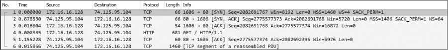
Figure 11-23: Packets 2 and 5 show high latency.

As we begin stepping through these six packets, we encounter our first sign of latency immediately. The initial SYN packet is sent by the client (172.16.16.128) to begin the TCP handshake, and a delay of 0.87 seconds is seen before the return SYN/ACK is received from the server (74.125.95.104). This is our first indicator that we are experiencing wire latency, which is caused by a device between the client and server.

We can make the determination that this is wire latency because of the nature of the types of packets being transmitted. When the server receives a SYN packet, a very minimal amount of processing is required to send a reply, because the workload doesn’t involve any processing above the transport layer. Even when a server is experiencing a very heavy traffic load, it will typically respond quickly to a SYN packet with a SYN/ACK. This eliminates the server as the potential cause of the high latency.

The client is also eliminated because, at this point, it is not doing any processing beyond simply receiving the SYN/ACK packet. Elimination of both the client and server points us to potential sources of slow communication within the first two packets of this capture.

Continuing, we see that the transmission of the ACK packet that completes the three-way handshake occurs quickly, as does the HTTP GET request sent by the client. All of the processing that generates these two packets occurs locally on the client following receipt of the SYN/ACK, so these two packets are expected to be transmitted quickly, as long as the client is not under a heavy processing load.

At packet 5, we see another packet with an incredibly high time value. It appears that after our initial HTTP GET request was sent, the ACK packet returned from the server took 1.15 seconds to be received. Upon receipt of the HTTP GET request, the server sent a TCP ACK before it began sending data, which once again requires very little processing by the server. This is another sign of wire latency.

Whenever you experience wire latency, you will almost always see it exhibited in both the SYN/ACK during the initial handshake and in other ACK packets throughout the communication. Although this information doesn’t tell you the exact source of the high latency on this network, it does tell you that neither client nor server is the source, so you know that the latency is due to some device in between. At this point, you could begin examining the various firewalls, routers, and proxies to locate the culprit.

Slow Communications: Client Latency

The next latency scenario we’ll examine is contained in latency3.pcapng, as shown in Figure 11-24.

Figure 11-24: The slow packet in this capture is the initial HTTP GET.

This capture begins normally, with the TCP handshake occurring very quickly and without any signs of latency. Everything appears to be fine until packet 4, which is an HTTP GET request after the handshake has completed. This packet shows a 1.34-second delay from the previously received packet.

To determine the source of this delay, we need to examine what is occurring between packets 3 and 4. Packet 3 is the final ACK in the TCP handshake sent from the client to the server, and packet 4 is the GET request sent from the client to the server. The common thread here is that these are both packets sent by the client and are independent of the server. The GET request should occur quickly after the ACK is sent, since all of these actions are centered on the client.

Unfortunately for the end user, the transition from ACK to GET doesn’t happen quickly. The creation and transmission of the GET packet requires processing up to the application layer, and the delay in this processing indicates that the client was unable to perform the action in a timely manner. Thus, the client is ultimately responsible for the high latency in the communication.

Slow Communications: Server Latency

The last latency scenario we’ll examine uses the file latency4.pcapng, as shown in Figure 11-25. This is an example of server latency.

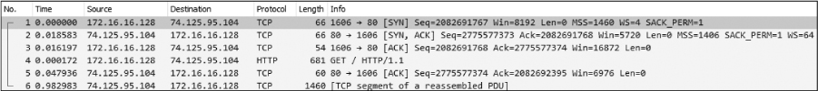
Figure 11-25: High latency isn’t exhibited until the last packet of this capture.

In this capture, the TCP handshake process between these two hosts completes flawlessly and quickly, so things begin well. The next couple of packets bring more good news, as the initial GET request and response ACK packets are delivered quickly as well. It is not until the last packet in this file that we see signs of high latency.

This sixth packet is the first HTTP data packet sent from the server in response to the GET request sent by the client, and it has a slow arrival time of 0.98 seconds after the server sends its TCP ACK for the GET request. The transition between packets 5 and 6 is very similar to the transition we saw in the previous scenario between the handshake ACK and GET request. However, in this case, the server is the focus of our concern.

Packet 5 is the ACK that the server sends in response to the GET request from the client. As soon as that packet has been sent, the server should begin sending data almost immediately. The accessing, packaging, and transmitting of the data in this packet is done by the HTTP protocol, and because this is an application-layer protocol, a bit of processing is required by the server. The delay in receipt of this packet indicates that the server was unable to process this data in a reasonable amount of time, ultimately pointing to it as the source of latency in this capture file.

Latency Locating Framework

Using six packets, we’ve managed to locate the source of high network latency between the client and the server in several scenarios. The diagram in Figure 11-26 should help you troubleshoot your own latency issues. These principles can be applied to almost any TCP-based communication.

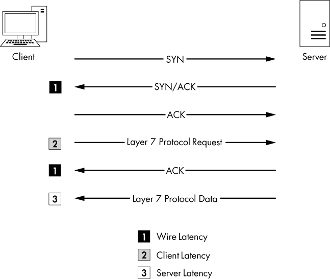
Figure 11-26: This diagram can be used to troubleshoot your own latency issues.

Network Baselining

When all else fails, your network baseline can be one of the most crucial pieces of data you have when troubleshooting slowness on the network. For our purposes, a network baseline consists of a sample of traffic from various points on the network that includes a large chunk of what we would consider “normal” network traffic. The goal of having a network baseline is for it to serve as a basis of comparison when the network or devices on it are misbehaving.

For example, consider a scenario in which several clients on the network complain of slowness when logging in to a local web application server. If you were to capture this traffic and compare it to a network baseline, you might find that the web server is responding normally but that the external DNS requests resulting from external content embedded in the web application are running twice as slowly as normal.

You might have noticed the slow external DNS server without the aid of a network baseline, but when you are dealing with subtle changes, that may not be the case. Ten DNS queries taking 0.1 seconds longer than normal to process are just as bad as one DNS query taking 1 full second longer than normal, but the former situation is much harder to detect without a network baseline.

Because no two networks are alike, the components of a network baseline can vary drastically. The following sections provide examples of the components of a network baseline. You may find that all of these items apply to your network infrastructure or that very few of them do. Regardless, you should be able to place each component of your baseline inside one of three basic baseline categories: site, host, and application.

Site Baseline

The purpose of the site baseline is to gain an overall snapshot of the traffic at each physical site on your network. Ideally, this would be every segment of the WAN.

Components of this baseline might include the following:

Protocols in Use

To see traffic from all devices, use the Protocol Hierarchy Statistics window (Statistics   ▶ Protocol Hierarchy) while capturing traffic from all the devices on the network segment at the network edge (router/firewall). Later, you can compare against the hierarchy output to find out whether normally present protocols are missing or new protocols have introduced themselves on the network. You can also use this output to find above ordinary amounts of certain types of traffic based on protocol.

Broadcast Traffic

This includes all broadcast traffic on the network segment. Sniffing at any point within the site should let you capture all of the broadcast traffic, allowing you to know who or what normally sends a lot of broadcast out on the network. Then you can quickly determine whether you have too much (or not enough) broadcasting going on.

Authentication Sequences

These include traffic from authentication processes on random clients to all services, such as Active Directory, web applications, and organization-specific software. Authentication is one area in which services are commonly slow. The baseline allows you to determine whether authentication is to blame for slow communications.

Data Transfer Rate

This usually consists of a measure of a large data transfer from the site to various other sites in the network. You can use the capture summary and graphing features of Wireshark (demonstrated in Chapter 5) to determine the transfer rate and consistency of the connection. This is probably the most important site baseline you can have. Whenever any connection entering or leaving the network segment seems slow, you can perform the same data transfer as in your baseline and compare the results. This will tell you whether the connection is actually slow and will possibly even help you find the area in which the slowness begins.

Host Baseline

You probably don’t need to baseline every single host within your network. The host baseline should be performed on only high-traffic or mission-critical servers. Basically, if a slow server will result in angry phone calls from management, you should have a baseline of that host.

Components of the host baseline include the following:

Protocols in Use

This baseline provides a good opportunity to use the Protocol Hierarchy Statistics window while capturing traffic from the host. Later, you can compare against this baseline to find out whether normally present protocols are missing or new protocols have introduced themselves on the host. You can also use this to find unusually large amounts of certain types of traffic based on protocol.

Idle/Busy Traffic

This baseline simply consists of general captures of normal operating traffic during peak and off-peak times. Knowing the number of connections and amount of bandwidth used by those connections at different times of the day will allow you to determine whether slowness is a result of user load or another issue.

Startup/Shutdown

To obtain this baseline, you’ll need to create a capture of the traffic generated during the startup and shutdown sequences of the host. If the computer refuses to boot, refuses to shut down, or is abnormally slow during either sequence, you can use this baseline to determine whether the cause is network related.

Authentication Sequences

Getting this baseline requires capturing traffic from authentication processes to all services on the host. Authentication is one area in which services are commonly slow. The baseline allows you to determine whether authentication is to blame for slow communications.

Associations/Dependencies

This baseline consists of a longer-duration capture to determine what other hosts this host is dependent upon (and are dependent upon this host). You can use the Conversations window (Statistics   ▶ Conversations) to see these associations and dependencies. An example is a SQL Server host on which a web server depends. We are not always aware of the underlying dependencies between hosts, so the host baseline can be used to determine these. From there, you can determine whether a host is not functioning properly due to a malfunctioning or high-latency dependency.

Application Baseline

The final network baseline category is the application baseline. This baseline should be performed on all business-critical network-based applications.

The following are the components of the application baseline:

Protocols in Use

Again, for this baseline, use the Protocol Hierarchy Statistics window in Wireshark, this time while capturing traffic from the host running the application. Later, you can compare against this list to find out whether protocols that the application depends on are functioning incorrectly or not at all.

Startup/Shutdown

This baseline includes a capture of the traffic generated during the startup and shutdown sequences of the application. If the application refuses to start or is abnormally slow during either sequence, you can use this baseline to determine the cause.

Associations/Dependencies

This baseline requires a longer-duration capture in which the Conversations window can be used to determine on which other hosts and applications this application depends. We are not always aware of the underlying dependencies between applications, so this baseline can be used to determine those. From there, you can determine whether an application is not functioning properly due to a malfunctioning or high-latency dependency.

Data Transfer Rate

You can use the capture summary and graphing features of Wireshark to determine the transfer rate and consistency of the connections to the application server during its normal operation. Whenever the application is reported as being slow, you can use this baseline to determine whether the issues being experienced are a result of high utilization or high user load.

Additional Notes on Baselines

Here are a few more points to keep in mind when creating your network baseline:

•     When creating your baselines, capture each one at least three times: once during a low-traffic time (early morning), once during a high-traffic time (midafternoon), and once during a no-traffic time (late night).

•     When possible, avoid capturing directly from the hosts you are baselining. During periods of high traffic, doing so may put an increased load on the device, hurt its performance, and cause your baseline to be invalid due to dropped packets.

•     Your baseline will contain some very intimate information about your network, so be sure to secure it. Store it in a safe place where only the appropriate individuals have access. But at the same time, keep it readily accessible so you can use it when needed. Consider keeping it on a USB flash drive or on an encrypted partition.

•     Keep all .pcap   and .pcapng files associated with your baseline and create a cheat sheet of the more commonly referenced values, such as associations or average data transfer rates.

Final Thoughts

This chapter has focused on troubleshooting slow networks. We’ve covered some of the more useful reliability detection and recovery features of TCP, demonstrated how to locate the source of high latency in network communications, and discussed the importance of a network baseline and some of its components. Using the techniques discussed here, along with some of Wireshark’s graphing and analysis features, you should be well equipped to troubleshoot when you get that call complaining that the network is slow.