5
ADVANCED WIRESHARK FEATURES

Once you master the basics of Wireshark, the next step is to delve into its analysis and graphing capabilities. In this chapter, we’ll look at some of these powerful features, including the Endpoints and Conversations windows, the finer points of name resolution, protocol dissection, stream interpretation, IO graphing, and more. These features, which are unique to Wireshark as a graphical analysis tool, are useful at multiple stages in the analysis process. Make sure to at least attempt to use all the features listed here before moving on, because we’ll revisit them frequently as we look at practical analysis scenarios throughout the rest of the book.

Endpoints and Network Conversations

For network communication to take place, data must be flowing between at least two devices. Each device sending or receiving data on the network represents what Wireshark calls an endpoint. The communication between two endpoints is called a conversation. Wireshark describes endpoints and conversations based on the attributes of the communication, specifically in terms of the addresses used within various protocols.

Endpoints are identified by multiple addresses, which are assigned at different layers of the OSI model. For example, at the data link layer, an endpoint will have a MAC address, which is a unique address built into the device (although it can be modified, potentially making it no longer required). At the network layer, however, the endpoint will have an IP address, which can be changed at any point. We’ll discuss in the next few chapters how these types of addresses are used.

Figure 5-1 shows two examples of how addresses are used to identify endpoints in conversations. Conversation A in the figure consists of two endpoints communicating at the data link (MAC) layer. Endpoint A has a MAC address of 00:ff:ac:ce:0b:de, and Endpoint B has a MAC address of 00:ff:ac:e0:dc:0f. Conversation B is defined by two devices communicating at the network (IP) layer. Endpoint A has an IP address of 192.168.1.25, and Endpoint B has an address of 192.168.1.30.

Figure 5-1: Endpoints and conversations on a network

Let’s look at how Wireshark can provide information about network communication on a per endpoint or conversation basis.

Viewing Endpoint Statistics

When analyzing traffic, you may find that you can pinpoint a problem as being at a specific endpoint on a network. For example, open the capture file lotsofweb.pcapng and open Wireshark’s Endpoints window (Statistics ▶ Endpoints). This window shows several helpful statistics for each endpoint, as shown in Figure 5-2, including the address, number of packets, and bytes transmitted and received.

Figure 5-2: The Endpoints window lets you view each endpoint in a capture file.

The tabs at the top of the window (TCP, Ethernet, IPv4, IPv6, and UDP) show the number of endpoints organized by protocol. To display only endpoints for a specific protocol, click one of these tabs. You can add additional protocol-filtering tabs by clicking the Endpoint Types box at the bottom right of the screen and selecting the protocol to add. If you would like to use name resolution to view endpoint addresses (see “Name Resolution” on page 84), check the Name resolution checkbox. If you’re dealing with a large capture and want to filter the endpoints displayed, you can apply a display filter in the main Wireshark window and select the Limit to display filter option in the Endpoints window. This option will make the window show only the endpoints matching the display filter.

Another handy feature of the Endpoints window is the ability to filter out specific packets for display in the Packet List pane. This is a quick way to drill down into the packets of an individual endpoint. Right-click an end-point to select the available filtering options. The dialog that appears will let you show or exclude packets related to the selected input. You can also choose the Colorize option in this dialog to export the endpoint address directly into a colorization rule (coloring rules are discussed in Chapter 4). In this way, you can quickly highlight packets related to a given endpoint so you can spot them quickly during analysis.

Viewing Network Conversations

With lotsofweb.pcapng still open, access the Wireshark Conversations window Statistics ▶ Conversations (Figure 5-3) to display all the conversations in the capture file. The Conversations window is similar to the Endpoints window, but the Conversations window shows two addresses per line to represent a conversation, as well as the packets and bytes transmitted to and from each device. The column Address A is the origin endpoint, and Address B is the destination.

Figure 5-3: The Conversations window lets you dissect each conversation in a capture file.

The Conversation window is organized by protocol. To see only conversations using a particular protocol, click one of the tabs at the top of the window (as with the Endpoints window) or add other protocol types by clicking the Conversation Types button at the lower right. As with the Endpoints window, you can use name resolution, limit the visible conversations using a display filter, and right-click a specific conversation to create filters based on specific conversations. Conversation-based filters are useful for digging into the details of interesting communication sequences.

Identifying Top Talkers with Endpoints and Conversations

The Endpoints and Conversations windows are helpful in network troubleshooting, especially when you’re trying to locate the source of a significant amount of traffic on the network.

As an example, let’s look again at lotsofweb.pcapng. As the name implies, this capture file contains HTTP traffic generated by multiple clients browsing the internet. Figure 5-4 shows a list of endpoints in this capture file sorted by number of bytes.

Notice that the endpoint responsible for the most traffic (by bytes) is the address 172.16.16.128. This is an internal network address (we’ll cover how that is determined in Chapter 7), and, as the device responsible for the most communication in this capture, it is given the designation top talker.

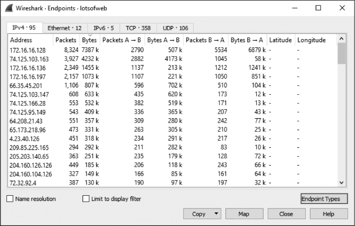
Figure 5-4: The Endpoints window shows which hosts are talking the most.

The address with the second highest amount of traffic is 74.125.103.163, an external (internet) address. When you encounter external addresses that you don’t know anything about, you can search the WHOIS registry to find the registered owner. In this case, the American Registry for Internet Numbers (https://whois.arin.net/ui/) reveals that Google owns this IP address, as seen in Figure 5-5.

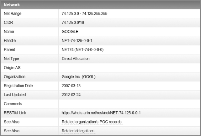
Figure 5-5: Viewing WHOIS results for 74.125.103.163 points to a Google IP.

Given this information, you could assume either that 172.16.16.128 and 74.125.103.163 are communicating a lot with multiple other devices on their own or that both endpoints are communicating with each other. In fact, as is often the case with top-talking endpoint pairs, the endpoints are communicating with each other. To confirm this, open the Conversations window, select the IPv4 tab, and sort the list by bytes. You should see that these two endpoints comprise the conversation with the highest number of transferred bytes. The pattern of transfer suggests a large download, because the number of bytes transmitted from external Address A (74.125.103.163) is much greater than the number of bytes transmitted from internal Address B (172.16.16.128), as shown in Figure 5-6.

Figure 5-6: The Conversations window confirms that the two top talkers are communicating with each other.

You can examine this conversation by applying this display filter:

ip.addr == 74.125.103.163 && ip.addr == 172.16.16.128

If you scroll through the list of packets, you’ll see several DNS requests to the youtube.com domain in the Info column of the Packet List window. This is consistent with our finding that 74.125.103.163 is a Google-owned IP address, because Google owns YouTube.

You’ll see how to use the Endpoints and Conversations windows in practical scenarios throughout the remaining chapters of this book.

Protocol Hierarchy Statistics

When dealing with unfamiliar capture files, you’ll sometimes need to determine the distribution of traffic by protocol. That is, what percentage of a capture is TCP, IP, DHCP, and so on? Rather than counting packets and totaling the results, Wireshark’s Protocol Hierarchy Statistics window can provide this information for you.

For example, with the lotsofweb.pcapng file still open and any previously applied filters cleared, open the Protocol Hierarchy Statistics window, as shown in Figure 5-7, by choosing Statistics ▶ Protocol Hierarchy.

Figure 5-7: The Protocol Hierarchy Statistics window shows the distribution of traffic by protocol.

The Protocol Hierarchy Statistics window gives you a snapshot of the type of activity occurring on a network. In Figure 5-7, 100 percent is Ethernet traffic, 99.7 percent is IPv4, 98 percent is TCP, and 13.5 percent is HTTP from web browsing. This information provides a great way to benchmark your network, especially once you have a mental picture of what your network traffic usually looks like. For instance, if you know that 10 percent of your network traffic is normally ARP traffic, but you see 50 percent ARP traffic in a recent capture, then something might be wrong. In some cases, the mere existence of a protocol could be of interest. If you don’t have any devices configured to use Spanning Tree Protocol (STP), seeing it in a protocol hierarchy might mean that a device is misconfigured.

Over time, you’ll find that you can use the Protocol Hierarchy Statistics window to profile the users and devices on a network simply by looking at the distribution of protocols in use. For example, a higher amount of HTTP traffic will tell you that there’s a lot of web browsing going on. You may also find that you can identify specific devices on the network simply by looking at the traffic from a network segment belonging to a business unit. For example, the IT department might use more administrative protocols such as ICMP or SNMP, customer service might be responsible for a high volume of SMTP (email) traffic, and the pesky intern in the corner might be flooding the network with World of Warcraft traffic!

Name Resolution

Network data is sent between endpoints with the help of various alphanumeric addressing systems that are often too long or complicated to remember, such as MAC address 00:16:ce:6e:8b:24, IPv4 address 192.168.47.122, or IPv6 address 2001:db8:a0b:12f0::1. Name resolution (also called name lookup) converts one identifying address into another, mostly for the sake of making the address easier to remember. For example, it’s much easier to remember google.com than to remember 216.58.217.238. By associating easy-to-read names with these cryptic addresses, we make them easier to remember and identify.

Enabling Name Resolution

Wireshark can use name resolution when it displays packet data to make analysis easier. To have Wireshark use name resolution, choose Edit ▶ Preferences ▶ Name Resolution. This window is shown in Figure 5-8. Here are the primary options available in Wireshark for name resolution:

Resolve MAC addresses   Uses the ARP protocol to attempt to convert layer 2 MAC addresses, such as 00:09:5b:01:02:03, into layer 3 addresses, such as 10.100.12.1. If attempts at these conversions fail, Wireshark will use the ethers file in its program directory to attempt conversion. Wireshark’s last resort is to convert the first 3 bytes of the MAC address into the device’s IEEE-specified manufacturer name, such as Netgear_01:02:03.

Resolve transport names   Attempts to convert a port number into a name associated with it, for example, to display port 80 as http. This is handy when you encounter an uncommon port and don’t know what service is typically associated with it.

Resolve network (IP) addresses   Attempts to convert a layer 3 address, such as 192.168.1.50, into an easy-to-read DNS name, such as MarketingPC1.domain.com. This is helpful for identifying the purpose or owner of a system, assuming it has a descriptive name.

Figure 5-8: Enabling name resolution in the Preferences dialog. Only Resolve MAC addresses is selected amongst the first three checkboxes pertaining to types of name resolution.

The Name Resolution preferences dialog in Figure 5-8 includes a few other useful options:

Use captured DNS packet data for address resolution   Parses DNS data from captured DNS packets to resolve IP addresses to DNS names.

Use an external network name resolver   Allows Wireshark to generate queries to the DNS server used by your analysis machine in order to resolve IP addresses to DNS names. This is helpful if you want to use DNS name resolution but the capture you are analyzing doesn’t contain the relevant DNS packets.

Maximum concurrent requests   Rate limits the number of concurrent DNS queries that can be outstanding at once. Use this option if your capture will generate a lot of DNS requests and you’re concerned about taking up too much bandwidth on your network or DNS server.

Only use the profile “hosts” file   Limits DNS resolution to the host file associated with the active Wireshark profile. I’ll describe how to use this file later in this section.

The changes made in the Preferences screen will persist after Wireshark is closed and reopened. To make name resolution changes on the fly without them being persistent, toggle name resolution settings on or off by clicking View ▶ Name Resolution on the main drop-down menu. You have the option of enabling or disabling name resolution for physical, transport, and network addresses.

You can leverage the various name resolution tools to make your capture files more readable and to save a lot of time in certain situations. For example, you can use DNS name resolution to help readily identify the name of a computer you are trying to pinpoint as the source of a particular packet.

Potential Drawbacks to Name Resolution

Given its benefits, using name resolution may seem like a no-brainer, but there are some potential drawbacks. First, network name resolution can fail if there is no DNS server available to provide the name associated with an IP address. Name resolution information is not saved with the capture file, so the resolution process must take place every time you open a file. If you capture packets on one network and then open the capture on another network, then your system might not be able to access the DNS servers from the source network and name resolution will fail.

In addition, name resolution requires additional processing overhead. When dealing with a very large capture file, you may want to forgo name resolution to conserve system resources. If you try to open a large capture and find your system struggling to load it or Wireshark crashes, disabling name resolution might help.

One further issue is that network name resolution’s reliance on DNS may generate unwanted packets that will cloud your capture file as traffic is sent to DNS servers to resolve addresses. Complicating things further, if the capture file you are analyzing contains malicious IP addresses, attempting to resolve them could generate queries to attacker-controlled infrastructure that could tip off an attacker that you are aware of their actions, possibly making you a target. To reduce the risk of clouding your packet file or of unwittingly communicating with an attacker, disable the Use an external network name resolver option in the Name Resolution Preferences dialog.

Using a Custom hosts File

It can be tedious to keep track of traffic from multiple hosts in large capture files, especially when external host resolution isn’t available. One way to help is to manually label systems based on their IP addresses with a Wireshark hosts file, which is a text file with a list of IP address to name mappings. You can use a hosts file to label addresses in Wireshark with names for quick reference. These names will be shown in the Packet List pane.

To use a hosts file, follow these steps:

1. Choose Edit ▶ Preferences ▶ Name Resolution and select Only use the profile “hosts” file.

2. Create a new file using Windows Notepad or a similar text editor. The file should contain one entry per line with an IP address and the name to resolve to, as shown in Figure 5-9. The name you choose on the right will be what is shown in the packet list window whenever Wireshark encounters the IP address on the left.

   

   Figure 5-9: Creating a Wireshark hosts file

3. Save the file as a plaintext file with the name hosts to the appropriate directory, as listed below. Be sure that the file has no extension!

   •     Windows: <USERPROFILE>Application DataWiresharkhosts

   •     OS X: /Users/<username>/.wireshark/hosts

   •     Linux: /home/<username>/.wireshark/hosts

Now open a capture, and any IP addresses in your hosts file should resolve to the specified names, as shown in Figure 5-10. Instead of IP addresses in the Source and Destination columns of the packet list window, more meaningful names are shown.

Figure 5-10: Name resolution from a hosts file in Wireshark

Using hosts files in this way can dramatically improve your ability to recognize certain hosts during analysis. When working with a team of analysts, consider sharing a hosts file of known assets among your networking staff. This will help your team quickly recognize systems with static addresses, such as servers and routers.

Manually Initiated Name Resolution

Wireshark also has the ability to force name resolution on a temporary, on-demand basis. This is done by right-clicking a packet in the Packet List pane and choosing the Edit Resolved Name option. The window that pops up will allow you to specify a name for an address, like a label. This resolution will be lost once the capture file is closed, making this a quick way to label an address without making any permanent changes that would have to be reverted later. I use this technique often because it is a little easier than manually editing a hosts file for every packet capture I look at.

Protocol Dissection

One of Wireshark’s biggest strengths is its support for the analysis of over a thousand protocols. Wireshark has this capability because it is open source, thus providing a framework for creating protocol dissectors. These allow Wireshark to recognize and decode a protocol into various fields so the protocol can be displayed in the user interface. Wireshark uses several dissectors in unison to interpret each packet. For example, the ICMP protocol dissector allows Wireshark to recognize that an IP packet contains ICMP data, pull out the ICMP type and code, and format those fields for display in the Info column of the Packet List pane.

You can think of a dissector as the translator between raw data and the Wireshark program. For a protocol to be supported by Wireshark, it must have a dissector (or you can write your own).

Changing the Dissector

Wireshark uses dissectors to detect individual protocols and decide how to display network information. Unfortunately, Wireshark doesn’t always make the right choices when selecting the dissector to use on a packet. This is especially true when a protocol on the network is using a nonstandard configuration, such as a non-default port (which is often configured by network administrators as a security precaution or by employees trying to circumvent access controls).

When Wireshark incorrectly applies dissectors, it’s possible to override this selection. For example, open the trace file wrongdissector.pcapng. This file contains a bunch of SSL communication between two computers. SSL is the Secure Socket Layer protocol, which is used for encrypted communication between hosts. Under most normal circumstances, viewing SSL traffic in Wireshark won’t yield much usable information due to its encrypted nature. However, there is something definitely wrong here. If you peruse the contents of several of these packets by clicking them and examining the Packet Bytes pane, you will find plaintext traffic. In fact, if you look at packet 4, you will find mention of the FileZilla FTP server application. The next few packets clearly display a request and response for both a username and a password.

If this were actually SSL traffic, you wouldn’t be able to read any of the data contained in the packets, and you certainly wouldn’t see all the user-names and passwords transmitted in clear text, as in Figure 5-11. Given the information shown here, it’s safe to assume that this is probably FTP traffic, rather than SSL traffic. Wireshark is likely interpreting this traffic as SSL because it is using port 443, as seen under the Info column, and port 443 is the standard port used for HTTPS (HTTP over SSL).

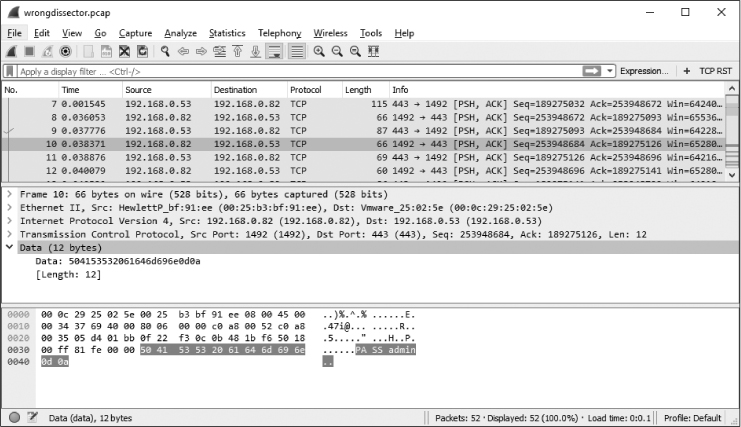
Figure 5-11: Plaintext usernames and passwords? This looks more like FTP than SSL!

To fix this problem, you can apply a forced decode to Wireshark to use the FTP protocol dissector on these packets. Here are the steps:

1. Right-click an SSL packet (such as packet 30) in the Protocol column and select Decode As, which opens a new dialog.

2. Tell Wireshark to decode all TCP port 443 traffic as FTP by selecting TCP port in the Field column, entering 443 in the Value column, and selecting FTP from the drop-down menu in the Current column, as shown in Figure 5-12.

   

   Figure 5-12: The Decode As... dialog allows you to create forced decodes.

3. Click OK to see the changes immediately applied to the capture file.

The data will be decoded as FTP traffic so you can analyze it from the Packet List pane without needing to dig deep into individual bytes (Figure 5-13).

Figure 5-13: Viewing properly decoded FTP traffic

The forced decode feature can be used multiple times in the same capture file. Wireshark will keep track of your forced decodes for you in the Decode As... dialog, where you can view and edit all of the forced decodes you have created so far.

By default, forced decodes are not saved when you close a capture. You can remedy this by clicking the Save button in the Decode As... dialog. This will save the protocol-decoding rules to your current Wireshark user profile; they will be applied when you open any capture using that profile. Saved decode rules can be removed by clicking the minus button in the dialog.

It’s very easy to save decoding rules and forget about them. This can lead to a lot of confusion when you aren’t prepared for it, so be mindful of forced decodes. To prevent myself from falling victim to this oversight, I generally avoid saving forced decodes to my primary Wireshark profile.

Viewing Dissector Source Code

The beauty of working with an open source application is that, if you are confused about why something is happening, you can look at the source code and find out why. This really comes in handy when you are trying to determine why a particular protocol has been interpreted incorrectly, because you can examine individual protocol dissectors.

Examining the source code of protocol dissectors can be done directly from the Wireshark website by clicking the Develop link and clicking Browse the Code. This link will send you to the Wireshark code repository, where you can view the release code for recent Wireshark versions. The protocol dissectors are in the epan/dissectors folder, and each dissector is labeled packets-<protocolname>.c.

These files can be rather complex, but they all follow a standard template and tend to be commented very well. You don’t need to be an expert C programmer to understand the basic function of each dissector. If you want to get a deep understanding of what you are seeing in Wireshark, I recommend taking a look at dissectors for some of the simpler protocols.

Following Streams

One of Wireshark’s most satisfying analysis features is its ability to reassemble data from multiple packets into a consolidated, easily readable format, often called a packet transcript. So you don’t have to view data being sent from client to server in a bunch of small chunks while clicking from packet to packet, stream following sorts the data to make it easier to view.

Four types of streams are available to follow:

TCP stream   Assembles data from protocols that utilize TCP, such as HTTP and FTP.

UDP stream   Assembles data from protocols that utilize UDP, such as DNS.

SSL stream   Assembles data from protocols that are encrypted, such as HTTPS. You must supply keys to decrypt the traffic.

HTTP stream   Assembles and decompresses data from the HTTP protocol. This is useful when following HTTP data via TCP stream doesn’t decode the HTTP payload fully.

As an example, consider a simple HTTP transaction in the file http_google.pcapng. Click any of the TCP or HTTP packets in the file, right-click the packet, and choose Follow TCP Stream. This will consolidate the TCP stream and open the conversation transcript in a separate window, as in Figure 5-14.

The text displayed in this window is in two colors, with red text (shown here with the lighter gray shading) signifying traffic from source to destination and blue text (shown here with the darker gray shading) identifying traffic in the opposite direction, from destination to source. The color relates to which side initiated the communication. In our example, the client initiated the connection to the web server, so it’s displayed in red.

The communication in the TCP stream begins with an initial GET request for the web root directory (/) and a response from the server that the request was successful in the form of an HTTP/1.1 200 OK. A similar pattern is repeated throughout other streams in the packet capture as the client requests individual files and the server responds with them. You are seeing a user browsing to the Google home page, but instead of having to step through every packet, you’re able to scroll through the transcript with ease. You’re actually seeing what the end user is seeing, but from the inside out.

Figure 5-14: The Follow TCP Stream window reassembles the communication in an easily readable format.

In addition to viewing the raw data in this window, you can search within the text; save it as a file; print it; or choose to view the data in ASCII, EBCDIC, hex, or C array format. These options, which make digging through larger sets of data easier, can be found at the bottom of the Follow Stream window.

Following SSL Streams

Following TCP and UDP streams is a simple two-click operation, but viewing SSL streams in a readable format requires a few additional steps. Because the traffic is encrypted, you are required to supply the private key associated with the server responsible for the encrypted traffic. The method you will use to retrieve this key varies depending on the server technology in use and is beyond the scope of this book, but once you have it, you will have to load it into Wireshark using the following process:

1. Access your Wireshark preferences by clicking Edit ▶ Preferences.

2. Expand the Protocols section and click the SSL protocol heading (shown in Figure 5-15). Click the Edit button next to the RSA keys list label.

3. Click the plus (+) button.

4. Supply the required information. This includes the IP address of the server responsible for the encryption, the port, the protocol, the location of the key file, and a password for the key file if one was used.

5. Restart Wireshark.

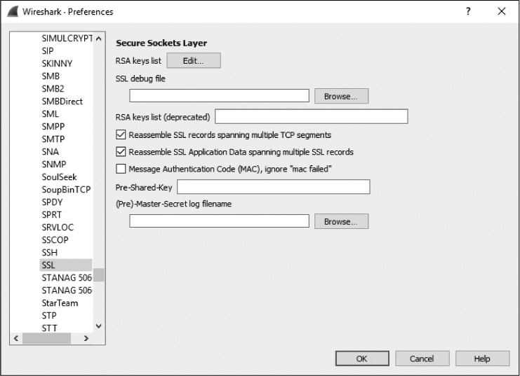
Figure 5-15: Adding SSL decryption information

Once this process is complete, you should be able to capture encrypted traffic between a client and server. Right-click an HTTPS packet and click Follow SSL Stream to see the clear text transcript.

The ability to view packet transcripts is one of the most commonly used analysis features in Wireshark, and you will come to rely on it to quickly determine what specific protocols are being used to do. We’ll cover several additional scenarios in later chapters that rely on viewing packet transcripts.

Packet Lengths

The size of a single packet or group of packets can tell you a lot about a situation. Under normal circumstances, the maximum size of a frame on an Ethernet network is 1,518 bytes. When you subtract the Ethernet, IP, and TCP headers from this number, you are left with 1,460 bytes that can be used for the transmission of a layer 7 protocol header or for data. If you know the minimum requirements for packet transmission, you can begin to look at the distribution of packet lengths in a capture to make educated guesses about the makeup of the traffic. This is immensely helpful for attempting to understand the composition of large capture files. Wireshark provides the Packet Lengths dialog for you to view the distribution of packets based on length.

Let’s look at an example by opening the file download-slow.pcapng. Once it is open, select Statistics ▶ Packet Lengths. The result is the Packet Lengths dialog shown in Figure 5-16.

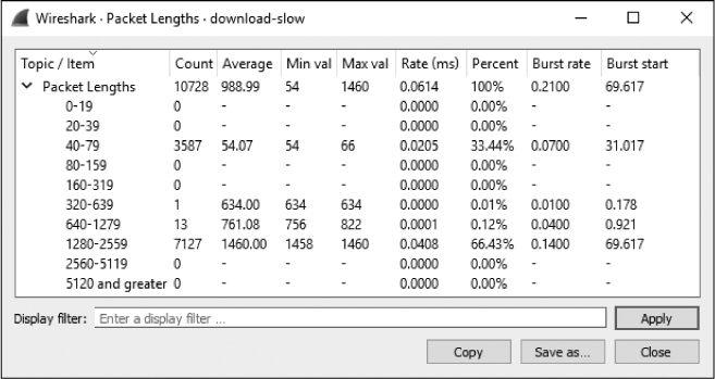
Figure 5-16: The Packet Lengths dialog helps you make educated guesses about the traffic in the capture file.

Pay special attention to the row showing statistics for packets ranging from 1,280 to 2,559 bytes. Larger packets like these typically indicate the transfer of data, whereas smaller packets indicate protocol control sequences. In this case, we have a large percentage of bigger packets (66.43 percent). Without seeing the packets in the file, we can make the educated guess that the capture contains one or more transfers of data. This could be in the form of an HTTP download, an FTP upload, or any other type of network communication in which data is transferred between hosts.

Most of the remaining packets (33.44 percent) are in the 40- to 79-byte range. Packets in this range are usually TCP control packets that don’t carry data. Let’s consider the typical size of protocol headers. The Ethernet header is 14 bytes (plus a 4-byte CRC), the IP header is a minimum of 20 bytes, and a TCP packet with no data or options is also 20 bytes. This means that standard TCP control packets—such as SYN, ACK, RST, and FIN packets—will be around 54 bytes and fall in this range. Of course, the addition of IP or TCP options will increase this size. We’ll dig into IP and TCP in Chapters 7 and 8, respectively.

Examining packet lengths is a great way to get a bird’s-eye view of a large capture. If there are a lot of large packets, it may be safe to assume that data is being transferred. If the majority of packets are small, indicating that not much data is being passed, you may assume that the capture consists of protocol control commands. These are not hard-and-fast rules, but making such assumptions is helpful before diving deeper.

Graphing

Graphs are the bread and butter of analysis and one of the best ways to get a summary overview of a data set. Wireshark includes several graphing features to assist in understanding capture data, the first of which are its IO graphing capabilities.

Viewing IO Graphs

Wireshark’s IO Graph window allows you to graph the throughput of data on a network. You can use such graphs to find spikes and lulls in data throughput, discover performance lags in individual protocols, and compare simultaneous data streams.

To view an example of the IO graph of a computer as it downloads a file from the internet, open download-fast.pcapng. Click any TCP packet to highlight it and then select Statistics ▶ IO Graph.

The IO Graph window shows a graphical view of the flow of data over time. In the example in Figure 5-17, you can see that the download this graph represents averages around 500 packets per second and stays somewhat consistent throughout its duration before tapering off at the end.

Figure 5-17: The IO graph of the fast download is mostly consistent.

Let’s compare this to an example of a slower download. Leaving the current file open, open download-slow.pcapng in another instance of Wireshark. Bring up the IO graph of this download, and you’ll see a much different story, as shown in Figure 5-18.

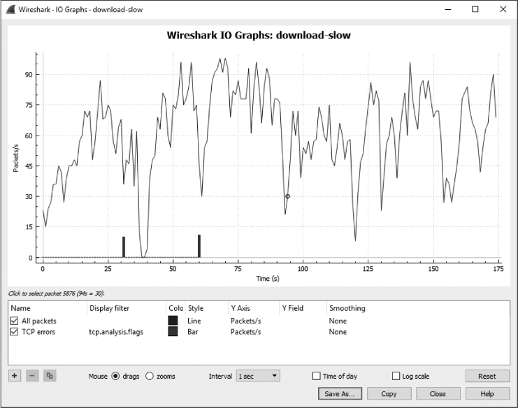
Figure 5-18: The IO graph of the slow download is not consistent at all.

This download has a transfer rate between 0 and 100 packets per second, and its rate is far from consistent, sometimes nearing 0 packets per second. You can see these inconsistencies more clearly if you place the IO graphs of the two files next to each other (see Figure 5-19). When comparing two graphs, pay attention to the x-and y-axis values to ensure that you’re comparing apples to apples. The scale will automatically adjust based on the number of packets and/or data transmitted, which is a key difference between the two graphs in Figure 5-19. The slower download shows a scale between 0 and 100 packets per second, while the faster download’s scale has a range of 0 to 700 packets per second.

Figure 5-19: Viewing multiple IO graphs side by side can be helpful in spotting variance.

The configurable options at the bottom of this window allow you to use multiple unique filters (using the same syntax as for a display or capture filter) and specify display colors for those filters. For instance, you can create filters for specific IP addresses and assign unique colors to them to view the variance in throughput for each device. Let’s try that out.

Open http_espn.pcapng, which was captured while a device was visiting the ESPN home page. If you look at the Conversations window, you’ll see that the top-talking external IP address is 205.234.218.129. From this, we can deduce that this host is likely the primary content provider we are receiving data from when visiting espn.com. However, there are also several other IPs participating in conversations, likely because additional content is being downloaded from external content providers and advertisers. We can show the disparity between the direct and third-party content delivery using the IO graph shown in Figure 5-20.

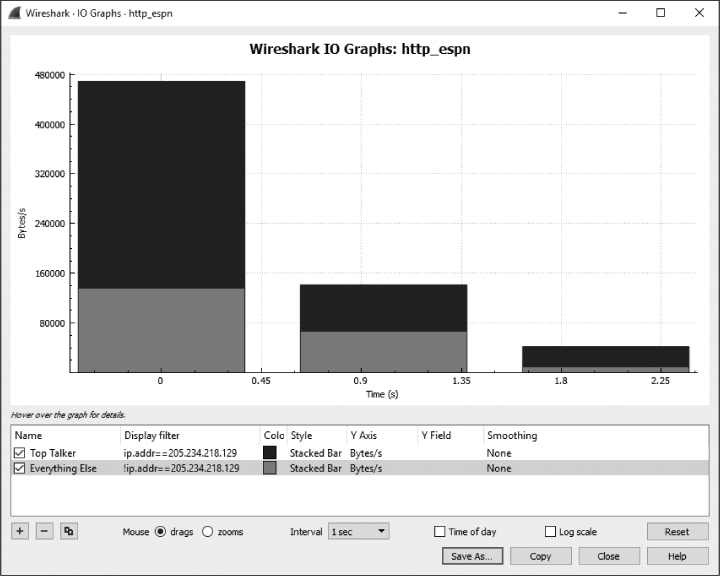
Figure 5-20: An IO graph showing IO of two separate devices.

The two filters applied in this chart are represented by the rows on the bottom of the IO Graph window. The filter named Top Talker shows IO only for the IP address 205.234.218.129, our primary content provider. It will graph this value in black using the stacked-bar style. The second filter, named Everything Else, will show IO for everything in the capture file except for the 205.234.218.129 address and thus includes all of the third-party content providers. This value will be graphed in red (shown here as the lighter gray) using the stacked bar. Notice that we’ve changed the y-axis unit to bytes per second. With these changes applied, it’s very easy to see the difference between primary and third-party content providers and just how much content is actually from a third-party source. This is a fun exercise to repeat on your frequently visited websites and a useful strategy for comparing the IO of different network hosts.

Round-Trip Time Graphing

Another graphing feature of Wireshark is the ability to view a plot of round-trip times for a given capture file. The round-trip time (RTT) is the time it takes for an acknowledgment to be received for a packet. Effectively, this is the time it took your packet to get to its destination and for the acknowledgment of that packet to be sent back to you. Analysis of RTTs is often done to find slow points or bottlenecks in communication and to determine whether there is any latency.

Let’s try out this feature. Open the file download-fast.pcapng. View the RTT graph of this file by selecting a TCP packet and then choosing Statistics ▶ TCP Stream Graphs ▶ Round Trip Time Graph. The RTT graph for download-fast.pcapng is shown in Figure 5-21.

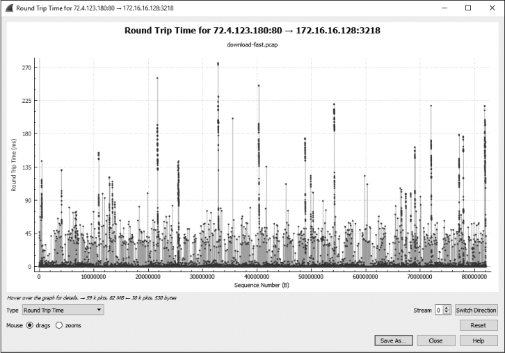
Figure 5-21: The RTT graph of the fast download appears mostly consistent, with only a few stray values.

Each point in the graph represents the RTT of a packet. The default view shows these values sorted by sequence number. You can click a plotted point within the graph to be taken directly to that packet in the Packet List pane.

It appears as though the RTT graph for the fast download has RTT values mostly under 0.05 seconds, with a few slower points between 0.10 and 0.25 seconds. Although there are quite a few higher values, the majority of the RTT values are okay, so this would be considered an acceptable RTT for a file download. When examining the RTT graph for throughput issues, you want to look for high latency times, which are indicated by multiple points plotted at higher y-axis values.

Flow Graphing

The flow graph feature is useful for visualizing connections and showing the flow of data over time, information that makes it easier to understand how devices are communicating. A flow graph contains a column-based view of a connection between hosts and organizes the traffic so you can interpret it visually.

To create a flow graph, open the file dns_recursivequery_server.pcapng and select Statistics ▶ Flow Graph. The resulting graph is shown in Figure 5-22.

Figure 5-22: The TCP flow graph allows us to visualize the connection much better.

This flow graph is a recursive DNS query, which is a DNS query that is received by one host and forwarded to another (we’ll cover DNS in Chapter 9). Each vertical line in the graph represents an individual host. The flow graph is a great way to visualize back-and-forth communication between two devices or, as in this example, the relationship between the communication of multiple devices. It’s also useful for understanding the normal flow of communication with protocols that you are less experienced with.

Expert Information

The dissectors for each protocol in Wireshark define expert info that can be used to alert you about particular states within packets of that protocol. These states are separated into four categories.

Chat   Basic information about the communication

Note   Unusual packets that may be part of normal communication

Warning   Unusual packets that are most likely not part of normal communication

Error   An error in a packet or the dissector interpreting it

For example, open the file download-slow.pcapng. Then click Analyze and select Expert Information to bring up the Expert Information window. Once there, deselect Group by summary to organize the output by severity (see Figure 5-23).

Figure 5-23: The Expert Information window shows information from the expert system programmed within the protocol dissectors.

The window has sections for each classification of information. Here there are no errors, 3 warnings, 19 notes, and 3 chats.

Most of the messages within this capture file are TCP related, simply because the expert information system has traditionally been most used with that protocol. At this time, there are 29 expert info messages configured for TCP, and they will be useful when you are troubleshooting capture files. These messages will flag an individual packet when it meets certain criteria, as listed below. (The meaning of these messages will become clearer as we study TCP in Chapter 8 and troubleshooting slow networks in Chapter 11.)

Chat Messages

Window Update   Sent by a receiver to notify a sender that the size of the TCP receive window has changed.

Note Messages

TCP Retransmission   Results from packet loss. Occurs when a duplicate ACK is received or the retransmission timer of a packet expires.

Duplicate ACK   When a host doesn’t receive the next sequence number it is expecting, it generates a duplicate ACK of the last data it received.

Zero Window Probe   Monitors the status of the TCP receive window after a zero window packet has been transmitted (covered in Chapter 11).

Keep Alive ACK   Sent in response to keep-alive packets.

Zero Window Probe ACK   Sent in response to zero-window-probe packets.

Window Is Full   Notifies a transmitting host that the receiver’s TCP receive window is full.

Warning Messages

Previous Segment Lost   Indicates packet loss. Occurs when an expected sequence number in a data stream is skipped.

ACKed Lost Packet   Occurs when an ACK packet is seen but the packet it is acknowledging is not.

Keep Alive   Triggered when a connection keep-alive packet is seen.

Zero Window   Seen when the size of the TCP receive window is reached and a zero window notice is sent out, requesting that the sender stop sending data.

Out-of-Order   Utilizes sequence numbers to detect when packets are received out of sequence.

Fast Retransmission   A retransmission that occurs within 20 milliseconds of a duplicate ACK.

Error Messages

No Error Messages

Although some of the features discussed in this chapter may seem as if they would be used only in obscure situations, you will probably find yourself using them more than you might expect. It’s important that you familiarize yourself with these windows and options; I will be referencing them a lot in the next few chapters.