
Chapter 6
Optimization Modeling
This chapter introduces optimization—a methodology for selecting an optimal strategy given an objective and a set of constraints. Optimization appears in a variety of financial applications, including portfolio allocation, trading strategies, identifying arbitrage opportunities, and pricing financial derivatives. In this chapter, we motivate the discussion with a simple example, and describe how optimization problems are formulated and solved.
Let us recall the retirement example from Chapter 5.2.3. We showed how to compute the realized return on the portfolio of stocks and bonds if we allocate 50% of the capital in each of the two investments. Can we obtain a “better” portfolio return with a different allocation? (As we discussed in Chapter 5, a “better” return is not well defined in the context of uncertainty, so for the sake of argument, let us assume that “better” means higher expected return.) We found that if the allocation in stocks and bonds is 30% and 70%, respectively, rather than 50% and 50%, we end up with a lower portfolio expected return, but also lower portfolio standard deviation. What about an allocation of (60%, 40%)? Of (80%, 20%)?
In this example, we are dealing with only two investments (the two asset classes), and we have no additional requirements on the portfolio structure. It is, however, still difficult to enumerate all the possibilities and find those that provide the optimal tradeoff of return and risk. In practice, portfolio managers are considering thousands of potential investments and need to worry about transaction costs, requirements on the portfolio composition, and trading constraints, which makes it impossible to find the “best” portfolio allocation by trial-and-error. The optimization methodology provides a disciplined way to approach the problem of optimal asset allocation. Problems such as the most cost-effective way to balance a portfolio can also be cast in the optimization framework.
6.1 Optimization Formulations
The increase in computational power and the tremendous pace of developments in the operations research field in the past 20 to 25 years has led to highly efficient algorithms and user-friendly software for solving optimization problems of many different kinds. To a large extent, the art of optimization modeling is in framing a situation so that the formulation fits within recognized frameworks for problem specifications, and can be passed to optimization solvers. It is important to understand the main building blocks of optimization formulations, as well as the limitations of the software and the insights that can be gained from the output of optimization solvers.
An optimization problem formulation consists of three parts:1
- A set of decision variables (usually represented as an
 –dimensional vector array2
  ),
), - An objective function, which is a function of the decision variables
 , and
, and - A set of constraints defined by functions
 of the general form
  (inequality constraints) and
  (equality constraints).
The decision variables are numerical quantities that represent the decisions to be made. In the portfolio example, the decision variables could be the portfolio weights. Alternatively, they could represent the dollar amount to allocate to each asset class. The objective function is a mathematical expression of the goal, and the constraints are mathematical expressions of the limitations in the business situation. In our example, the objective function could be an expression that computes the expected portfolio return, and the constraints could include an expression that computes the total portfolio risk. We can then maximize the expression of the objective function subject to an upper limit on the risk we are willing to tolerate.
Optimization software expects users to specify all three components of an optimization problem, although it is sometimes possible to have optimization problems with no constraints. The latter kind of optimization problems is referred to as unconstrained optimization. Unconstrained optimization problems are typically solved with standard techniques from calculus,3 and the optimal solution is selected from all possible points in the N-dimensional space of the decision variables x. When there are constraints, only some points in that space will be feasible, that is, only some will satisfy the constraints. The values of the decision variables that are feasible and result in the best value for the objective function are called the optimal solution. Optimization solvers typically return only one optimal solution. However, it is possible to have multiple optimal solutions, that is, multiple feasible solutions x that produce the same optimal value for the objective function.4
When formulating optimization problems, it is important to realize that the decision variables need to participate in the mathematical expressions for the objective function and the constraints that are passed to an optimization solver. Optimization algorithms then tweak the values of the decision variables in these expressions in a smart, computationally efficient way in order to produce the best value for the objective function with values for the decision variables that satisfy all of the constraints. In other words, we cannot simply pass the expression
to an optimization solver, unless Portfolio Expected Return is expressed as a function of the decision variables (the portfolio weights). As we show in Chapter 8, the expected portfolio return can be expressed in terms of the portfolio weights as ![]() , where
, where ![]() and
and ![]() are N-dimensional arrays containing the weights and the expected returns of the N assets in the portfolio, respectively. So, the objective function should be written as
are N-dimensional arrays containing the weights and the expected returns of the N assets in the portfolio, respectively. So, the objective function should be written as
which is interpreted as “maximize the value of ![]() over the possible values for
over the possible values for ![]() .”
.”
In addition, the input data in a classical optimization problem formulation need to be fixed numbers, not random variables. For example, the objective function of an optimization problem cannot be passed to a solver as
where Portfolio Return = ![]() , and
, and ![]() is the N-dimensional array with (uncertain) asset returns with some probability distributions. Some areas in optimization, such as robust optimization and stochastic programming, study methodologies for solving optimization problems in which the input data are subject to uncertainty and follow theoretical or empirical probability distributions. However, in the end, the methods for solving such problems reduce to specifying the coefficients in the optimization problem as fixed numbers that are representative of the underlying probability distributions.
is the N-dimensional array with (uncertain) asset returns with some probability distributions. Some areas in optimization, such as robust optimization and stochastic programming, study methodologies for solving optimization problems in which the input data are subject to uncertainty and follow theoretical or empirical probability distributions. However, in the end, the methods for solving such problems reduce to specifying the coefficients in the optimization problem as fixed numbers that are representative of the underlying probability distributions.
6.1.1 Minimization versus Maximization
Most generally, optimization solvers require an optimization problem formulation to be of the kind

There are variations on this formulation, and some have to do with whether the optimization problem falls in a specific class. (We discuss different categories of optimization problems based on the form of their objective function and the shape of their feasible set in Section 6.2.) Some optimization software syntax allows for specifying only minimization problems, while other optimization software packages are more flexible, and accept both minimization and maximization problems.
Standard formulation requirements are not as restrictive as they appear at first sight. For example, an optimization problem that involves finding the maximum of a function ![]() can be recast as a minimization problem by minimizing the expression
can be recast as a minimization problem by minimizing the expression ![]() , and vice versa: an optimization problem that involves finding the minimum of a function
, and vice versa: an optimization problem that involves finding the minimum of a function ![]() can be recast as a maximization problem by maximizing the expression
can be recast as a maximization problem by maximizing the expression ![]() . To obtain the actual value of the objective function, one then flips the sign of the optimal value. Exhibit 6.1 illustrates the situation for a quadratic function of one variable
. To obtain the actual value of the objective function, one then flips the sign of the optimal value. Exhibit 6.1 illustrates the situation for a quadratic function of one variable ![]() . The optimal value for
. The optimal value for ![]() is obtained at the optimal solution x*. The optimal value for
is obtained at the optimal solution x*. The optimal value for ![]() is obtained at
is obtained at ![]() as well. It also holds that
as well. It also holds that

Exhibit 6.1 An example of the optimal objective function values for  and
and  for a quadratic objective function
  of a single decision variable x.
For the portfolio expected return maximization example above, stating the objective function as
or
will produce the same optimal values for the decision variables ![]() . To get the actual optimal objective function value for
. To get the actual optimal objective function value for ![]() , we would flip the sign of the optimal objective function value obtained after minimizing
, we would flip the sign of the optimal objective function value obtained after minimizing ![]() .
.
6.1.2 Local versus Global Optima
In optimization, we distinguish between two types of optimal solutions: global and local optimal solutions. A global optimal solution is the “best” solution for any value of the decision variables vector ![]() in the set of all feasible solutions. A local optimal solution is the best solution in a neighborhood of feasible solutions. In the latter case, the objective function value at any point “close” to a local optimal solution is worse than the objective function value at the local optimal solution. Exhibit 6.2 illustrates the global (point A) and local (point B) optimal solution for the unconstrained minimization of a function of two variables.
in the set of all feasible solutions. A local optimal solution is the best solution in a neighborhood of feasible solutions. In the latter case, the objective function value at any point “close” to a local optimal solution is worse than the objective function value at the local optimal solution. Exhibit 6.2 illustrates the global (point A) and local (point B) optimal solution for the unconstrained minimization of a function of two variables.

Exhibit 6.2 Global (point A) versus local (point B) minimum for a function of two variables x1 and x2.
Most classical optimization algorithms can only find local optima. They start at a point, and go through solutions in a direction in which the objective function value improves. Their performance has an element of luck that has to do with picking a good starting point for the algorithm. For example, if a nonlinear optimization algorithm starts at point C in Exhibit 6.2, it may find the local minimum B first, and never get to the global minimum A. In the general case, finding the global optimal solution can be difficult and time consuming, and involves finding all local optimal solutions first, and then picking the best one among them.
The good news is that in some cases, optimization algorithms can explore the special structure of the objective function and the constraints to deliver stronger results. In addition, for some categories of optimization problems, a local optimal solution is in fact guaranteed to be the global optimal solution, and many optimization problems in finance have that property. (We review the most important kinds of such “nice” optimization problems in Section 6.2.) This makes the ability to recognize the type of optimization problem in a given situation and to formulate the optimization problem in a way that enables optimization algorithms to take advantage of the special problem structure even more critical.
6.1.3 Multiple Objectives
In practice, one often encounters situations in which one would like to optimize several objectives at the same time. For example, a portfolio manager may want to maximize the portfolio expected return and positive skew while minimizing the portfolio variance and kurtosis. There is no straightforward way to pass several objectives to an optimization solver. A multiobjective optimization problem needs to be reformulated as an optimization problem with a single objective. There are two commonly used methods to do this. The first is to assign weights to the different objectives, and optimize the weighted sum of objectives as a single objective function. The second is to optimize the most important objective, and include the other objectives as constraints, after assigning to each of them a bound on the value one is willing to tolerate.
6.2 Important Types of Optimization Problems
Optimization problems can be categorized based on the form of their objective function and constraints as well as the kind of decision variables. The type of optimization problem with which one is faced determines what software is appropriate, the efficiency of the algorithm for solving the problem, and the degree to which the optimal solution returned by the optimization solver is trustworthy and useful. Awareness of this fact is particularly helpful in situations in which there are multiple ways to formulate the optimization problem. The way in which one states the formulation will determine whether the optimization solver can exploit any special structure in the problem and achieve stronger results.
6.2.1 Convex Programming
As we mentioned in Section 6.1.2, some general optimization problems have “nice” structure in the sense that a local optimal solution is guaranteed to be the global optimal solution. Convex optimization problems have that property. A general convex optimization problem is of the form

where both ![]() and
and ![]() are convex functions and
are convex functions and ![]() is a system of linear equalities. A convex function of a single variable x has the shape in Exhibit 6.3(a). For a convex function, a line that connects any two points on the curve is always above the curve. The “opposite” of a convex function is a concave function (see Exhibit 6.3[b]), which looks like a “cave.” For a concave function, a line that connects any two points on the curve is always below the curve.
is a system of linear equalities. A convex function of a single variable x has the shape in Exhibit 6.3(a). For a convex function, a line that connects any two points on the curve is always above the curve. The “opposite” of a convex function is a concave function (see Exhibit 6.3[b]), which looks like a “cave.” For a concave function, a line that connects any two points on the curve is always below the curve.

Exhibit 6.3 Examples of (a) a convex function; (b) a concave function.
Convex programming problems encompass several classes of problems with special structure, including linear programming (LP), some quadratic programming (QP), second-order cone programming (SOCP), and semidefinite programming (SDP). Algorithms for solving convex optimization problems are more efficient than algorithms for solving general nonlinear problems but it is important to keep in mind that even within the class of convex problems, some convex problems are computationally more challenging than others. LP problems are best studied and easiest to solve with commercial solvers, followed by convex QP problems, SOCP problems, and SDP problems.
We introduce LP, QP, and SOCP in more detail next. Many classical problems in finance involve linear and quadratic programming, including asset-liability problems, portfolio allocation problems, and some financial derivative pricing applications. SDP problems are advanced formulations that have become more widely used in financial applications with recent advances in the field of robust optimization. They are beyond the scope of this book, but we refer interested readers to Fabozzi, Kolm, Pachamanova, and Focardi (2007) for a detailed overview of robust optimization formulations.
6.2.2 Linear Programming
Linear programming refers to optimization problems in which both the objective function and the constraints are linear expressions in the decision variables.5 The standard formulation statement for linear optimization problems is

All optimization problems involving linear expressions for the objective function and the decision variables can be converted to this standard form. We will see an example in Section 6.3.
Linear optimization problems are the easiest kind of problems to solve. Modern specialized optimization software can handle LP formulations with hundreds of thousands of decision variables and constraints in a matter of seconds. In addition, linear optimization problems belong to the class of convex problems for which a local optimal solution is guaranteed to be the global optimal solution. (We discuss this in more detail in Section 6.4.) LPs arise in a number of finance applications, such as asset allocation among asset classes, the construction of portfolios of securities within an asset class, and identification of arbitrage opportunities. The sample optimization problem formulation we provide in Section 6.3 is a linear optimization problem.
6.2.3 Quadratic Programming
Quadratic programming problems have an objective function that is a quadratic expression in the decision variables and constraints that are linear expressions in the decision variables. The standard form of a quadratic optimization problem is

where ![]() is an N-dimensional vector of decision variables as before, and the other arrays are input data:
is an N-dimensional vector of decision variables as before, and the other arrays are input data:
 is an
is an  matrix,
 is an N-dimensional vector,
 is a
is a  matrix,
 is a J-dimensional vector.
When the matrix ![]() is positive semi-definite,6 the objective function is convex. (It is a sum of a convex quadratic term and a linear function, and a linear function is both convex and concave.) Since the objective function is convex and the constraints are linear expressions, we have a convex optimization problem. The problem can be solved by efficient algorithms, and we can trust that any local optimum they find is in fact the global optimum. When
is positive semi-definite,6 the objective function is convex. (It is a sum of a convex quadratic term and a linear function, and a linear function is both convex and concave.) Since the objective function is convex and the constraints are linear expressions, we have a convex optimization problem. The problem can be solved by efficient algorithms, and we can trust that any local optimum they find is in fact the global optimum. When ![]() is not positive semi-definite, however, the quadratic problem can have several local optimal solutions and stationary points, and is therefore more difficult to solve.
is not positive semi-definite, however, the quadratic problem can have several local optimal solutions and stationary points, and is therefore more difficult to solve.
The most prominent use of quadratic programming in finance is for asset allocation and trading models. We will see examples in Chapter 8.
6.2.4 Second-Order Cone Programming
Second-order cone programs (SOCPs) have the general form

where ![]() is an N-dimensional vector of decision variables as before and the other arrays are input data:
is an N-dimensional vector of decision variables as before and the other arrays are input data:
 is an N-dimensional vector,
 is a
is a  matrix,
 is a J-dimensional vector,
 are
are  matrices,
 are Ii-dimensional vectors,
 are scalars.
The notation ![]() stands for second norm, or Euclidean norm. (It is sometimes denoted
stands for second norm, or Euclidean norm. (It is sometimes denoted ![]() to differentiate it from other types of norms.) The Euclidean norm of an N-dimensional vector
to differentiate it from other types of norms.) The Euclidean norm of an N-dimensional vector ![]() is defined as7
is defined as7
The SOCP class of problems is more general than the classes covered in Sections 6.2.2 and 6.2.3. LPs, convex QPs, and convex problems with quadratic objective function and quadratic constraints can be reformulated as SOCPs with some algebra.
It turns out that SOCP problems share many nice properties with linear programs, so algorithms for their optimization are very efficient. SOCP formulations in finance arise mostly in robust optimization applications. We discuss such formulations in Chapter 7.
6.2.5 Integer and Mixed Integer Programming
So far, we have classified optimization problems according to the form of the objective function and the constraints. Optimization problems can be classified also according to the type of decision variables ![]() . Namely, when the decision variables are restricted to be integer (or, more generally, discrete) values, we refer to the corresponding optimization problem as an integer programming (IP) or a discrete problem. When some decision variables are discrete and some are continuous, we refer to the optimization problem as a mixed integer programming (MIP) problem. In special cases of integer problems in which the decision variables can only take values 0 or 1, we refer to the optimization problem as a binary optimization problem.
. Namely, when the decision variables are restricted to be integer (or, more generally, discrete) values, we refer to the corresponding optimization problem as an integer programming (IP) or a discrete problem. When some decision variables are discrete and some are continuous, we refer to the optimization problem as a mixed integer programming (MIP) problem. In special cases of integer problems in which the decision variables can only take values 0 or 1, we refer to the optimization problem as a binary optimization problem.
Integer and mixed integer optimization formulations are useful for formulating extensions to classical portfolio allocation problems. Index-tracking formulations and many constraints on portfolio structure faced by managers in practice require modeling with discrete decision variables. Examples of constraints include maximum number of assets to be held in the portfolio (so-called cardinality constraints), maximum number of trades, round-lot constraints (constraints on the size of the orders in which assets can be traded in the market),8 and fixed transaction costs. We discuss such formulations further in Chapter 11.
6.3 A Simple Optimization Problem Formulation Example: Portfolio Allocation
To provide better intuition for how optimization problems are formulated, we give a simplified example of an asset allocation problem formulation. We will see more advanced nonlinear problems formulations in the context of portfolio applications in Chapters 8 and 11.
We explain the derivation of the optimization problem formulation in detail, so that the process of optimization problem formulation can be explicitly outlined. The problem formulation is the crucial step—once we are able to map a situation to one of the optimization problem types reviewed in Section 6.2, we can find the optimal solution with optimization software. Later in this chapter, we explain how optimization formulations can be input into a solver, and how the output can be retrieved and interpreted.
Suppose that the portfolio manager at a large university in the United States is tasked with investing a $10 million donation to the university endowment. He has decided to invest these funds only in mutual funds9 and is considering the following four types of mutual funds: an aggressive growth fund (Fund 1), an index fund (Fund 2), a corporate bond fund (Fund 3), and a money market fund (Fund 4), each with a different expected annual return and risk level.10 The investment guidelines established by the Board of Trustees limit the percentage of the funds that can be allocated to any single type of investment to 40% of the total amount. The data for the portfolio manager's task are provided in Exhibit 6.4. In addition, in order to contain the risk of the investment to an acceptable level, the amount of money allocated to the aggressive growth and the corporate bond funds cannot exceed 60% of the portfolio, and the aggregate average risk level of the portfolio cannot exceed 2. What is the optimal portfolio allocation for achieving the maximum expected return at the end of the year if no short selling is allowed?11
Exhibit 6.4 Data for the portfolio manager's problem.
| Fund Type | Growth | Index | Bond | Money Market |
| Fund # | 1 | 2 | 3 | 4 |
| Expected return | 20.69% | 5.87% | 10.52% | 2.43% |
| Risk level | 4 | 2 | 2 | 1 |
| Max investment | 40% | 40% | 40% | 40% |
To formulate the optimization problem, the first thing we need to ask is what the objective is. In this case, the logical objective is to maximize the expected portfolio return. The second step is to think of how to define the decision variables. The decision variables need to be specified in such a way as to allow for expressing the objective as a mathematical expression of the quantities the manager can control to achieve his objective. The latter point is obvious, but sometimes missed when formulating optimization problems for the first time. For example, although the market return on the assets is variable and increasing market returns will increase the portfolio's return, changing the behavior of the market is not under the manager's control. The manager, however, can change the amounts he invests in different assets in order to achieve his objective.12 Thus, the vector of decision variables can be defined as
Let the vector of expected returns be ![]() . Then, the objective function can be written as
. Then, the objective function can be written as
It is always a good idea to write down the actual description and the units for the decision variables, the objective function, and the constraints. For example, the units of the objective function value in this example are dollars.
Finally, there are several constraints.
- The total amount invested should be $10 million. This can be formulated as
 .
. - The total amount invested in Fund 1 and Fund 3 cannot be more than 60% of the total investment ($6 million). This can be written as

-
The average risk level of the portfolio cannot be more than 2. This constraint can be expressed as
4*(proportion of investment with risk level 4) + 2*(proportion of investment with risk level 2) + 1*(proportion of investment with risk level 1) ≤ 2 or, mathematically, as

Note that this is not a linear constraint. (We are dividing decision variables by decision variables.) Based on our discussion in Section 6.2, from a computational perspective, it is better to have linear constraints whenever we can. There are different ways to convert this particular constraint into a linear constraint. For example, we can multiply both sides of the inequality by
 , which is a nonnegative number and will preserve the sign of the inequality as is. In addition, in this particular example we know that the total amount
  , so the constraint can be formulated as
- The maximum investment in each fund cannot be more than 40% of the total amount ($4,000,000). These constraints can be written as

-
Finally, given the no-short-selling requirement, the amounts invested in each fund cannot be negative. (Note we are assuming that the portfolio manager can invest only the $10,000,000, and cannot borrow additional money.)

These are nonnegativity constraints. Even though they seem obvious in this example, they still need to be specified explicitly for the optimization solver.
The final optimization formulation can be written in matrix form. The objective function is

Let us organize the constraints together into groups according to their signs. (This will be useful when we discuss solving the problem with optimization software later.)


This problem is an LP. It would look like the standard form in Section 6.2.2, except for the inequality ![]() constraints. We can rewrite the LP in standard form by converting them to equality constraints. We introduce six additional nonnegative variables
constraints. We can rewrite the LP in standard form by converting them to equality constraints. We introduce six additional nonnegative variables ![]() (called slack variables), one for each constraint in the group Inequality
(called slack variables), one for each constraint in the group Inequality ![]() :
:

Then, we add the nonnegativity constraints on the slack variables to the problem formulation:
Optimization solvers in the past required that the problem be passed in standard form; however, solvers and optimization languages are much more flexible today, and do their own conversion to standard form. In any case, as this example illustrates, it is easy to go from a general linear problem formulation to the standard form.
6.4 Optimization Algorithms
How do optimization solvers actually find the optimal solution for a problem? As a general rule, optimization algorithms are iterative. They start with an initial solution and generate a sequence of intermediate solutions until they get “close” to the optimal solution. The degree of “closeness” is determined by a parameter called tolerance, which usually has some default value, but can often be modified by the user. Often, the tolerance parameter is linked to a measure of the distance between the current and the subsequent solution, or to the incremental progress made by subsequent iterations of the algorithm in improving the objective function value. If subsequent iterations of the algorithm bring very little change relative to the status quo, the algorithm is terminated.
The algorithms for optimization in today's optimization software are rather sophisticated and an extensive introduction to these algorithms is beyond the scope of this book. However, many optimization solvers let the user select which optimization algorithm to apply to a specific problem, and some basic knowledge of what algorithms are used for different classes of optimization solvers is helpful for deciding what optimization software to use and what options to select for the problem at hand.
The first optimization algorithm, called the simplex algorithm, was developed by George Dantzig in 1947. It finds optimal solutions to linear optimization problems by iteratively solving systems of linear equations to find intermediate feasible solutions in a way that continually improves the value of the objective function. Despite its age, the simplex algorithm is still widely used for linear optimization, and is remarkably efficient in practice.
In the 1980s, inspired by a new algorithm Narendra Karmakar created for linear programming problems, another class of efficient algorithms called interior point methods was developed. The advantage of interior point methods is that they can be applied not only to linear optimization problems but also to a wider class of convex optimization problems.
Many nonlinear optimization algorithms are based on using information from a special set of equations that represent necessary conditions that a solution x is optimal. These conditions are the Karush-Kuhn-Tucker (KKT) conditions for optimality. The KKT conditions for a solution x* to be the optimum are necessary but not sufficient, meaning that they need to be satisfied at the optimal solution; however, a solution that satisfies them is not necessarily the global optimum. Hence, the user is not guaranteed that the solution returned by the optimization algorithm is indeed the global optimum solution. The KKT conditions are, fortunately, necessary and sufficient for optimality in the case of convex optimization problems. They take a special form in the case of linear optimization problems and some other classes of convex problems, which is exploited in interior point algorithms for finding the optimal solution.
The importance of the KKT conditions for general nonlinear optimization is that they enable a nonlinear optimization problem to be reduced to a system of nonlinear equations, whose solution can be attained by using successive approximations. Widely used algorithms for nonlinear optimization include barrier methods, primal-dual interior point methods, and sequential quadratic programming methods. The latter try to solve the KKT conditions for the original nonlinear problem by optimizing a quadratic approximation to a function derived from the objective function and the constraints of the original problem.13
Integer programming problems, that is, problems with integer decision variables, are typically solved by branch-and-bound algorithms, branch-and-cut routines, and heuristics14 that exploit the special structure of the problem.15 The main idea behind many of these algorithms is to start by solving a relaxation of the optimization problem in which the decision variables are not restricted to be integer numbers. The algorithms then begin with the solution found in the initial stage and narrow down the choices of integer solutions. In practice, a simple rounding of the initial fractional optimal solution is sometimes good enough. However, it can lead to an integer solution that is very far from the actual optimal solution, and the problem is more pronounced when the number of integer decision variables is large.
Integer programming problems are generally more difficult and take longer to solve than problems with continuous decision variables. In addition, not every optimization solver can handle them, so it is important to check the specifications of the solver before trying to solve such problems. There are some good commercial optimization solvers that can handle linear and convex quadratic mixed-integer optimization problems, but there are virtually no solvers that can handle more general nonlinear mixed-integer problems efficiently.
A number of algorithms incorporate an element of randomness in their search. Specifically, they allow moves to feasible solutions with worse value of the objective function to happen with some probability, rather than pursuing always a direction in which the objective function improves. Although there are no guarantees, the hope is that this will prevent the algorithm from getting stuck in a local optimum so that the algorithm finds the global optimum in the case of multiple local optima.
Randomized search algorithms for optimization fall into several classes, including simulated annealing, tabu search, and genetic algorithms. Genetic algorithms in particular have become an option in several popular Microsoft Excel add-ins for optimization, such as Premium Solver and Palisade's Evolver. Package GA in R16 is designed for optimization using genetic algorithms. MATLAB also has a Genetic Algorithms and Direct Search Toolbox, which contains simulated annealing and genetic algorithms.
Randomized search algorithms have their drawbacks—they can be slow, and provide no guarantee that they will find the global optimum. However, they are appropriate for handling difficult integer problems, nonlinear problems, and problems with discontinuities, when traditional optimization solvers fail.
6.5 Optimization Software
When selecting an optimization software product, it is important to differentiate between optimization solvers and optimization modeling languages.
An optimization solver is software that implements numerical routines for finding the optimal solution of an optimization problem. Well-known commercial optimization solvers include MOSEK17 and IBM ILOG CPLEX18 for linear, mixed-integer, and quadratic problems, and MINOS, SNOPT, and CONOPT for general nonlinear problems,19 but there are a number of other commercial and free solvers available.
Optimization modeling languages have emerged as user-friendly platforms that allow the user to specify optimization problems in a more intuitive generic fashion, regardless of the specific algorithmic and input requirements of optimization routines. Typically, optimization language software automates the underlying mathematical details of the optimization model formulation, but does not actually solve the problem. It passes the formulation to a solver, and retrieves the results from the solver in a convenient format. Popular optimization languages include AMPL20 and GAMS.21 The Computational Infrastructure for Operations Research22 project (COIN-OR, or simply COIN) is a great resource for information about solvers and modeling languages available for optimization.
Optimization solvers and modeling languages are often part of modeling environments that handle not only the optimization, but also the input and output processing, statistical analysis, and perform other functions a user may need for a comprehensive analysis of a situation. MATLAB is an example of a high-level technical computing and interactive environment for model development that also enables data visualization, data analysis, and numerical simulation. The optimization solvers in MATLAB's Optimization Toolbox can solve a variety of constrained and unconstrained optimization problems for linear programming, quadratic programming, nonlinear optimization, and binary integer programming. Other examples of modeling environments include IBM ILOG OPL Studio, which allows users to build optimization models that are then accessed from a subroutine library using VBA, Java, or C/C++. Thus, a user can connect optimization systems directly to data sources, and make calls to optimization subroutines repeatedly.
Free open-source alternatives for modeling environments include R23 and Python.24 Although such open source alternatives may not always be as user-friendly as commercial alternatives, they have the advantage that new algorithms are constantly developed and implemented by contributors to the projects, and sometimes one can find functionality that commercial software companies have not yet had the time to develop.
Excel's inherent capabilities for optimization are rather limited. Excel Solver, which ships with Excel, can handle only optimization problems of small size, up to a few hundred variables and constraints. It is a perfectly acceptable solver for linear optimization problems, but its performance (and the output one would obtain from it) is unreliable for more complex problems of the general nonlinear or integer programming type. Premium Solver Platform,25 which is sold by the developers of Excel Solver, is an extended and improved version of the standard Excel Solver, and can handle linear, integer, and quadratic problems of larger size. It employs efficient interior point methods for solving classical optimization formulations and genetic algorithms for arbitrary Excel optimization models that contain spreadsheet functions such as IF, INDEX, and COUNTIF (such functions are not recognized in traditional optimization problem formulations). Palisade's Evolver is another add-in for Excel that uses genetic algorithms to solve optimization problems. The Palisade Decision Tools Suite26 also contains RiskOptimizer, which is a tool for optimization given possible scenarios for the uncertain parameters in the problem. Premium Solver Platform is part of Analytics Solver Platform,27 which also offers tools for statistics, simulation, and data mining. Analytics Solver Platform and Palisade's Decision Tools Suite are examples of modeling environments for Excel: they contain a number of software add-ins for optimization, statistical analysis, and sensitivity analysis that use a spreadsheet program—MS Excel—as the underlying platform.
It should be mentioned that there are numerous optimization software packages that target financial applications in particular, especially portfolio management applications. Established vendors of portfolio management software include Axioma,28 MSCI Barra,29 ITG,30 and Northfield Information Services.31 More recently, traditional financial data providers such as Bloomberg and FactSet have added portfolio optimization capabilities to their offerings. Bloomberg introduced Portfolio Optimizer to its Portfolio and Risk Analytics Platform and fully integrated it with the data feeds. FactSet offers the ability to integrate its data feeds with portfolio optimization software vendors such as Axioma, MSCI Barra, and Northfield.
6.6 A Software Implementation Example
Modeling environments employ very different approaches to the formulation and output formatting of optimization problems. For example, array-based modeling languages like R and MATLAB expect optimization formulations to be passed to solvers in an array form, and contain functions that call specific solvers for specific types of optimization problems. In particular, R has a number of application programming interfaces (commonly referred to as APIs) to both commercial and free optimization solvers.32 Examples of APIs for leading commercial packages include cplexAPI33 and Rcplex34 (an interface to the CPLEX optimization package from IBM) and Rmosek35 (an interface to the MOSEK solver). Free optimization packages for R include linprog36 (for linear programming) and quadprog (for quadratic programming, which is often used in portfolio optimization), as well as the package Rglpk,37 which provides an interface to the free GNU Linear Programming Kit.38
Optimization modeling with spreadsheets requires a different approach. Microsoft Excel's Solver and other Excel optimization add-ins use spreadsheet values and formulas as inputs, and return output to the spreadsheet.
In order to provide a concrete example, in this section we show how the portfolio allocation problem from Section 6.3 can be formulated and solved with Excel Solver. We begin with a general description of how optimization works with Excel Solver, and then show the specific inputs and outputs for the portfolio allocation example.
6.6.1 Optimization with Excel Solver
Excel Solver comes prepackaged with Excel.39 Its main dialog box is shown in Exhibit 6.5. Excel Solver expects users to input an objective cell, changing variable cells, and constraints, and specify whether the optimization problem is a maximization or a minimization problem.

Exhibit 6.5 Excel Solver dialog box.
The entry for the objective cell should be a reference to a cell that contains a formula for the objective function of the optimization problem. This formula should link the objective cell and the changing variable cells. The changing variable cells are cells dedicated to the decision variables—they can be left empty, or have some initial values that the solver will eventually replace with the optimal values. The initial values of the changing variable cells are used by Solver as the starting point of the algorithm. They do not really matter when the optimization problem is linear, but they can cause Solver to find very different solutions if the problem is nonlinear or contains integer variables.
Constraints can be specified by clicking on the Add button, then entering the left-hand side and the right-hand side of a constraint, as well as the sign of the constraint. The constraint dialog box is shown in Exhibit 6.6. By clicking on the middle button, the user can specify inequality constraints (≤ or ≥) or equality constraints (=). Solver also lets the user specify whether a set of decision variables is integer (int) or binary (bin). To do that, the user must have designated the cells corresponding to these decision variables as changing cells, and then add the int or bin constraint through the Add Constraint dialog box. The last option, dif, stands for “alldifferent.” It imposes the constraint that if there are N decision variables (changing variable cells), they all take different integer values between 1 and ![]() .
.

Exhibit 6.6 Solver constraint dialog box.
Solver expects constraints to be entered as cell comparisons, that is, it can only compare the value of one cell to the value of another cell in the spreadsheet. One cannot type a formula directly into the constraint dialog box—the formula needs to be already contained in the cell that is referenced. A good way to organize an optimization formulation in Excel is to create a column of cells containing the formulas on the left-hand side of all constraints, and a column of cells containing the right-hand sides (the limits) of all constraints. That allows for groups of constraints to be entered simultaneously. For example, if there are three constraints that all have equal signs, one can enter an array reference to the range of three cells with the left-hand sides of these constraints, and an array reference to the range of three cells with the right-hand sides. Solver will compare each cell in the first array to the corresponding cell in the second array.
Solver also allows users to specify options for the algorithms it uses to find the optimal solution. This can be done by clicking on the Select a Solving Method drop-down menu as well as on the Options button in Solver's main dialog box. The Select a Solving Method drop-down menu is shown in Exhibit 6.5, and the Options dialog box is shown in Exhibit 6.7. For most problems, leaving the defaults in works fine; however, it is always helpful to provide as much information to the solver as possible to ensure optimal performance. For example, if we know that the optimization problem is linear, we should select Simplex LP from the Select a Solving Method drop-down menu. (GRG Nonlinear is a more general solver for nonlinear optimization problems, and Evolutionary is a solver based on genetic algorithms which use some randomization to find better solutions for difficult types of optimization models, such as problems with integer variables.)

Exhibit 6.7 Excel Solver Options dialog box.
The Make Unconstrained Variables Nonnegative option is a shortcut to declaring all decision variables nonnegative (rather than entering separate constraints for each decision variable). The Show Iteration Results option in the Options dialog box lets the user step through the search for the optimal solution. The Use Automatic Scaling option is helpful when there is big difference between the magnitudes of decision variables and input data, because sometimes that leads to computational issues due to poor scaling. An optimization problem is poorly scaled if changes in the decision variables produce large changes in the objective or constraint functions for some components of the vector of decision variables more than for others. (For example, if we are trying to find the optimal percentages to invest, but the rest of the data in the problem is measured in millions of dollars, the solver may run into numerical difficulties because a small change in a value measured in percentages will have a very different magnitude than a small change in a value measured in millions.) Some optimization techniques are very sensitive to poor scaling. In that case, checking the Use Automatic Scaling option instructs it to scale the data so the effect can be minimized.
The remaining options in the Options dialog box have to do with the numerical details of the algorithm used, and can be left at their default values. For example, Max Time lets the user specify the maximum amount of time for the algorithm to run in search of the optimal solution.
6.6.2 Solution to the Portfolio Allocation Example
Let us now solve the portfolio allocation problem in Section 6.3. Exhibit 6.8 shows a snapshot of an Excel spreadsheet with the model.

Exhibit 6.8 Snapshot of an Excel model of the portfolio allocation example from Section 6.3.
Cells B4:E4 are dedicated to storage of the values of the decision variables, and will be the changing variable cells for Solver. It is convenient then to keep the column corresponding to each variable dedicated to storing data for that particular variable. For example, row 7 contains the coefficients in front of each decision variable in the objective function (the expected returns). Similarly, the cell array B10:E16 contains the coefficients in front of each variable in each constraint in the problem. Cells H10:H16 contain the right-hand side limits of all constraints. (In fact, we are entering the data in matrix form.)
In cell F7, we enter the formula for calculating the objective function value in terms of the decision variables:
=SUMPRODUCT($B$4:$E$4,B7:E7)The SUMPRODUCT function in Excel takes as inputs two arrays, and returns the sum of the products of the corresponding elements in each array. In this case, the SUMPRODUCT formula is equivalent to the formula
=B7*B4+C7*C4+D7*D4+E7*E4but the SUMPRODUCT formula is clearly a lot more efficient to enter, especially when there are more decision variables.
Cells F10:F16 contain the formulas for the left-hand sides of the seven constraints. For example, cell F10 contains the formula
=SUMPRODUCT($B$4:$E$4,B10:E10)Now the advantage of organizing the data in this array form in the spreadsheet is apparent. When creating the optimization model, we can copy the formula in cell F10 down to all cells until cell F16. Thus, we can enter the information for multiple constraints very quickly.
We select Data | Solver, and enter the information in Exhibit 6.9.
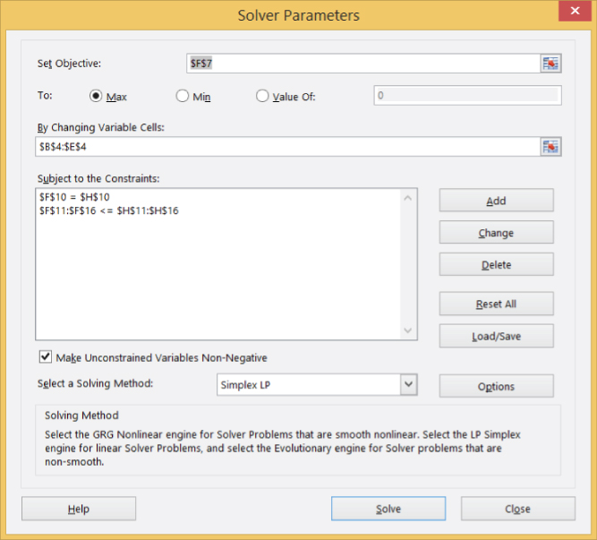
Exhibit 6.9 Excel Solver inputs for the portfolio allocation problem.
Our goal is to maximize the expression stored in cell F7 by changing the values in cells B4:E4, subject to a set of constraints. Note that since all constraints in rows 11–16 have the same sign (≥), we can pass them to Solver as one entry. Solver interprets the constraint
$F$11:$F$16 <= $H$11:$H$16equivalently to the set of constraints
$F$11<= $H$11
$F$12<= $H$12
$F$13<= $H$13
$F$14<= $H$14
$F$15<= $H$15
$F$16<= $H$16
We use the Simplex LP and the Make Unconstrained Variables Nonnegative options. The optimal solution is contained in the spreadsheet snapshot in Exhibit 6.8. To attain the optimal return of $931,800 while satisfying all required constraints, the manager should invest $2,000,000 in Fund 1, $0 in Fund 2, $4,000,000 in Fund 3, and $4,000,000 in Fund 4.