
Chapter 4
Statistical Estimation Models
When modeling portfolio risk, one can think about the distribution of financial returns at a particular point in time. This is the approach we took in Chapter 3—we reviewed probability distributions that can be used to represent observed characteristics of financial returns. A complementary approach is to use statistical models for asset return dynamics. Such models do not look at returns at a particular point in time in isolation—they identify factors that drive returns, or model the asset price process over time.
In this chapter, we review the most widely used statistical estimation models in portfolio management and explain how they are estimated and applied. We begin with a general discussion about return estimation models in finance followed by a review of linear regression analysis, factor analysis, and principal components analysis. We then discuss ARCH and GARCH models. The level of the chapter is intended to be introductory, and the emphasis is specifically on concepts that are useful in portfolio construction.1
4.1 Commonly Used Return Estimation Models
By far the most widely used return models in finance are models of the form
where
| is the rate of return on security i, | |
| is the sensitivity of asset i to factor k, | |
| is a constant, and | |
| is a random shock. |
The models are a mathematical expression of the assumption that financial return movements can be represented as a sum of predictable movements based on factor influences and a random (white) noise or error term. Despite their simple form, such models have remarkable flexibility. A fundamental model of this type is the regression model in which the values of all variables are recorded at the same time period and the random shock ![]() follows a normal distribution, making
follows a normal distribution, making ![]() normally distributed as well. This is a classical static regression model, which is often used to explain asset returns in terms of factors. Such factors can be macroeconomic variables (gross domestic product, level of interest rates) and/or company fundamentals (industry group, various financial ratios), and we discuss them in more detail in Chapter 9.
normally distributed as well. This is a classical static regression model, which is often used to explain asset returns in terms of factors. Such factors can be macroeconomic variables (gross domestic product, level of interest rates) and/or company fundamentals (industry group, various financial ratios), and we discuss them in more detail in Chapter 9.
In regression models, the factors are identified by the modeler, and a hypothesis is tested to verify that these factors explain returns in a statistically significant way. Two other kinds of statistical models covered in this chapter—factor analysis and principal component analysis—look very similar in terms of the equation estimated for returns; however, they extract factors from the data and do not treat them as exogenous.
The form of the model above is linear,2 which makes its estimation easier. However, nonlinear relationships between factors and the response variable (in this context, returns) can be incorporated as well. For example, the factors in the model can be modeled as nonlinear functions (such as a square or a logarithm) of observable variables.
The models can be made dynamic, too. For example, it may take some time for the market to respond to a change in a macroeconomic variable. The lag is measured in a certain number of time units, such as five months or two weeks. To incorporate such dynamics, one can include lagged values of factors in the equation above. Lagged values are values realized a certain number of time periods before the current time period. An example model of this kind is one in which the return on an asset i is determined by factor values from one time period ago (note the addition of the subscript t to the variables in the equation):
and a special model of this kind is one in which the return on an asset is determined by its own return values between 1 and p time periods ago:
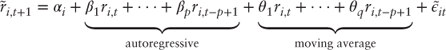
This is an autoregressive (AR) model of order p, a special case of the more general ARMA(p,q) (AutoRegressive Moving Average) model, which incorporates both lag terms and moving average3 terms:
Dynamics can be incorporated in the expectation of factor models as well, by assuming an autoregressive model for the factors themselves.4 Finally, one can incorporate dynamics in the white noise term ![]() . ARCH and GARCH models do just that, allowing for some important observed characteristics (“stylized facts”) of asset returns such as heavy tails and volatility clustering to be incorporated in the models.
. ARCH and GARCH models do just that, allowing for some important observed characteristics (“stylized facts”) of asset returns such as heavy tails and volatility clustering to be incorporated in the models.
4.2 Regression Analysis
In regression analysis, a modeler specifies the factors that are thought to drive the co-variation in asset returns, and the statistical analysis confirms or rejects this hypothesis. As explained in the introduction, a regression equation assumes that the return on a particular stock i can be represented as
where
| is the mean return, | |
| are the K factors, | |
| are the coefficients in front of the factors, and | |
| is the residual error. |
In practice, the linearity assumption is not very restrictive, because nonlinear relationships can be represented by transforming the data as explained earlier.
The factors ![]() in this regression are the explanatory variables (also called independent or predictor variables). They help explain the variability in the response variable (also called dependent variable)
in this regression are the explanatory variables (also called independent or predictor variables). They help explain the variability in the response variable (also called dependent variable) ![]() .
.
4.2.1 A Simple Regression Example
Let us consider a simple example of a regression model with a single explanatory variable. Suppose we are trying to understand how the returns of a stock, say Procter & Gamble (P&G), are impacted by the returns of a market index (the S&P 500).5 The model we are trying to estimate looks as follows:
where ![]() is the return on P&G stock and
is the return on P&G stock and ![]() is the return on the S&P 500. The data used for the estimation are pairs of observations for the explanatory variable
is the return on the S&P 500. The data used for the estimation are pairs of observations for the explanatory variable ![]() and the response variable
and the response variable ![]() . Suppose there are
. Suppose there are ![]() such pairs of monthly observations. The data can be represented in a graph, referred to as a scatterplot, like the one in Exhibit 4.1, where the coordinates of each point are the observed values of the two variables (
such pairs of monthly observations. The data can be represented in a graph, referred to as a scatterplot, like the one in Exhibit 4.1, where the coordinates of each point are the observed values of the two variables (![]() and
and ![]() ).
).

Exhibit 4.1 Determining a linear relationship between returns on a market index (the S&P 500) and returns on P&G stock.
Building the model requires finding coefficients α and β so that the line determined by the regression equation is “as close” as possible to all the observations. There are different measures of proximity but the classical measure is that the sum of the squared deviations from all the points (observations) to the line is the smallest possible. This is referred to as an ordinary least squares (OLS) regression. The line obtained using the OLS regression is plotted in Exhibit 4.1.
Because linear regression is the most fundamental statistical estimation model, virtually every statistical package (and many not specifically statistical ones such as Excel) contains functions for estimating a regression model. The only inputs one needs to specify are which variable is the response and which variable(s) are the explanatory variables. The calculations for the regression model output typically use the OLS method, where the formula for calculating the parameters is derived using calculus to minimize the sum of squared residuals from the regression, or maximum likelihood estimation, which maximizes a log-likelihood function.6 Even though the output formats for different statistical packages differ, the information conveyed in them is standard, so we will use the Excel output in Exhibit 4.2 to discuss the most important terminology associated with regression models.

Exhibit 4.2 Excel regression output for the P&G example.
The value for the coefficient beta in front of the explanatory variable (the S&P 500 excess return in our example) is 0.4617 (cell B18). This value tells us the amount of change in the response variable when the explanatory variable increases by one unit. (In a regression with multiple explanatory variables, this interpretation is still valid if we hold the values of the other explanatory variables constant.) In this case, the return of the P&G stock will change by about half (0.4617) of the amount of change in the return on the S&P 500.
The value of the intercept alpha is ![]() (cell B17). The intercept tells us the value of the response variable if the values for all explanatory variables are zero.
(cell B17). The intercept tells us the value of the response variable if the values for all explanatory variables are zero.
The estimated model equation based on this regression is
For example, if the monthly return on the S&P 500 is 0.0400, we would expect the return on P&G to be, on average, ![]() . Before this model can be used, however, it needs to be validated by testing for statistical significance and explanatory power. We show how this is done next.
. Before this model can be used, however, it needs to be validated by testing for statistical significance and explanatory power. We show how this is done next.
If the regression coefficient beta is statistically different from 0, the explanatory variable to which the regression coefficient corresponds will be significant for explaining the response variable. To check whether the regression coefficient is statistically significant (which means that it is statistically different from zero), we can check its p-value (cell E18) or the confidence interval associated with the coefficient (cells F18:G18). If the p-value is small (generally, less than 5% is considered small enough), then the beta coefficient is statistically different from zero. In this example, the p-value is 0.0000040709 (=4.0709·10–6, or 4.0709E-06 in Excel's notation), which is very small, so we can conclude that the S&P 500 excess return is a significant factor for forecasting P&G's stock returns. The same conclusion can be reached by checking whether zero is contained in the confidence interval for the regression coefficient. In this case, the 95% confidence interval for beta is (0.2766, 0.6468). Zero is not contained in the interval; therefore, the beta coefficient is statistically different from zero, and the S&P 500 return is a significant factor for explaining the P&G stock returns.
There are several other statistics we should consider in evaluating the regression model. The p-value for the F-statistic (cell F12), which in Excel appears as “Significance F,” tells us whether the regression model as a whole is statistically significant. Because in our example the p-value for the F-statistic is small (0.0000040709), the regression model is significant.
Three measures of goodness of fit are reported as standard output for a regression. The coefficient of determination ![]() (which in Excel appears as “R Square” in cell B5) tells us what percentage of the variability of the response variable is explained by the explanatory variable. The higher the number is, the better. (It ranges from 0% to 100%.) In this example, 24.51% of the variability in P&G returns can be explained by the variability in the S&P 500 returns. The problem with
(which in Excel appears as “R Square” in cell B5) tells us what percentage of the variability of the response variable is explained by the explanatory variable. The higher the number is, the better. (It ranges from 0% to 100%.) In this example, 24.51% of the variability in P&G returns can be explained by the variability in the S&P 500 returns. The problem with ![]() is that if we add more explanatory variables (factors),
is that if we add more explanatory variables (factors), ![]() will stay the same or continue to increase, even if the additional factors are not important. To control for this, in multiple regression models one looks also at the Adjusted
will stay the same or continue to increase, even if the additional factors are not important. To control for this, in multiple regression models one looks also at the Adjusted ![]() (cell B6), which imposes a penalty for having too many explanatory variables.
(cell B6), which imposes a penalty for having too many explanatory variables.
Another measure of goodness of fit is the standard error of the regression (cell B7), which equals the standard deviation of the regression residuals, the errors left after the model is fitted. The units of the standard error are the units of the residuals, which are also the units of the response variable. In our example, a standard error of 0.0403 tells us that the forecasts for the S&P 500 returns based on this regression model will be on average 0.0403 off from the observed S&P 500 returns.
In order for the regression model to be valid, we need to check that three assumptions that are made in regression analysis regarding the residuals (ε) are satisfied:
- Assumption 1: The residuals ε follow a normal distribution.
- Assumption 2: The residuals ε exhibit homoscedasticity (i.e., they have the same variability regardless of the values of the response and the explanatory variables).
- Assumption 3: The residuals ε are not autocorrelated (i.e., they do not exhibit patterns that depend on the order of the data in the data set).
Assumption 1 can be checked visually by creating a histogram of the residuals from the regression, and examining whether the distribution is bell-shaped and close to a normal curve fitted to the distribution (with the same mean and variance). One can also use a normal probability plot or quantile–quantile (Q-Q) plot that shows the standardized values of the residuals from the regression against the corresponding quantile values for a standard normal distribution.
Assumption 2 can be checked visually from graphs of the residuals against the response variable values predicted from the regression as well as against individual explanatory variables. A fan-shaped pattern with residuals farther away from the fitted regression line as, say, values for the response variable increase, is a typical indication that the homoscedasticity assumption is not satisfied by the regression model.
Assumption 3 can be checked visually by plotting a time series of the residuals from the regression. With observations collected over time, a cyclical pattern, for example, would indicate autocorrelation. In addition, the Durbin-Watson statistic or the Dickey-Fuller test are often used to evaluate the degree of autocorrelation in the residuals.
Many statistical software packages produce graphs and summary metrics that allow for checking these assumptions as part of the standard regression output. When the assumptions are not satisfied, the modeling exercise is not completed, since one may be able to improve the explanatory power of the model. One should consider
- Transforming the explanatory variables by using functions such as logarithm, square, square root (this may fix the statistical problems associated with the violation of the first two assumptions about the residuals).
- Incorporating lagged explanatory variables or modeling the changing variability of the error term explicitly (this may fix the statistical problems associated with the last two assumptions about the residuals).
In regression models with multiple explanatory variables, we are also concerned about multicollinearity, which happens when the explanatory variables are highly correlated among themselves. In the specific context of forecasting asset returns, an example of factors that could be correlated, for example, is the level of interest rates and stock market returns, or credit spreads and stock market returns. Strong correlation between the factors means that it is difficult to isolate the effect of one variable from the effect of the other. This makes the estimates of the regression coefficients (the betas) misleading because they can take on multiple values, it inflates the value of the ![]() of the regression artificially, and leads to estimates for the p-values and other measures of the significance of the regression coefficients that cannot be trusted.7 To check for multicollinearity, one examines the correlation matrix of the explanatory variables and other measures of co-dependence such as the variance inflation factors (VIFs), which are standard output in more advanced statistical packages. Unfortunately, there is not much that can be done if multicollinearity is observed. Sometimes, explanatory variables can be dropped or transformed.
of the regression artificially, and leads to estimates for the p-values and other measures of the significance of the regression coefficients that cannot be trusted.7 To check for multicollinearity, one examines the correlation matrix of the explanatory variables and other measures of co-dependence such as the variance inflation factors (VIFs), which are standard output in more advanced statistical packages. Unfortunately, there is not much that can be done if multicollinearity is observed. Sometimes, explanatory variables can be dropped or transformed.
Finally, when we build regression models, there is a trade-off between finding a model with good explanatory power and parsimony (i.e., limiting the number of factors that go into the model). On the one hand, we want to include all factors that are significant for explaining the response variable (in many finance applications, this is typically returns). On the other hand, including too many factors requires collecting a lot of data, and increases the risk of problems with the regression model, such as multicollinearity.
4.2.2 Regression Applications in the Investment Management Process
Regression analysis is the workhorse of quantitative finance. It is used in virtually every stage of the quantitative equity investment management process, as well as in a number of interesting bond portfolio applications. This section provides a brief overview of the applications of regression in the four stages of the investment management process described in Chapter 1.
4.2.2.1 Setting an Investment Policy
Setting an investment policy begins with the asset allocation decision. Although there is a wide variety of asset allocation models, they all require the expected returns for different asset classes. (Some, like the Markowitz mean-variance model we describe in Chapter 8, require also the variances and covariances.) These expected returns and other inputs are typically calculated using regression analysis. We explain the estimation process in more detail in Chapter 9 but here we mention that the regression models that are used establish links between returns and their lagged values or exogenous variables. These variables are referred to as “factors.” The justification for the models that are used is primarily empirical, that is, they are considered valid insofar as they fit empirical data.
4.2.2.2 Selecting a Portfolio Strategy
Clients can request a money manager for a particular asset class to pursue an active (also referred to as alpha) or passive (also referred to as beta) strategy. As we explained in Chapter 1, an active portfolio strategy uses available information and forecasting techniques to seek a better performance than a portfolio that is simply diversified broadly. A passive portfolio strategy involves minimal input when it comes to forecasts, and instead relies on diversification to match the performance of some market index. There are also hybrid strategies.
Whether a client selects an active or a passive strategy depends on his or her belief that the market is efficient for an asset class. If the market is not efficient, the client needs to believe that the manager will be able to outperform the benchmark for the asset class that is believed to be inefficient. Regression analysis is used in most tests of the pricing efficiency of the market. The tests examine whether it is possible to generate abnormal returns. An abnormal return is defined as the difference between the actual return and the expected return from an investment strategy. The expected return used in empirical tests is the return predicted from a regression model after adjustment for transaction costs. The model itself adjusts for risk. To show price inefficiency, the abnormal return (or alpha) must be shown to be statistically significant.8
4.2.2.3 Selecting the Specific Assets
Given a portfolio strategy, portfolio construction involves the selection of the specific assets to be included in the portfolio. This step in the investment management process requires an estimate of expected returns as well as the variance and covariances of returns. Regression analysis is often used to identify factors that impact asset returns. In bond portfolio management, regression-based durations (key measures of interest rate exposures) are estimated to evaluate portfolio risk. Regression-based durations can be estimated also for equities. These are important, for example, in the case of defined-benefit pension funds, which match the duration of their asset portfolio to the duration of their pension liabilities. We explain some of these concepts in more detail in later chapters.
4.2.2.4 Measuring and Evaluating Performance
In evaluating the performance of a money manager, one must adjust for the risks accepted by the manager in generating the return. Regression (factor) models provide such information. The process of decomposing the performance of a money manager relative to each factor that has been found through multifactor models is called return (or performance) attribution analysis.
4.3 Factor Analysis
To illustrate the main idea behind factor analysis, let us begin with a simple nonfinance example provided by Kritzman (1993). Suppose that we have the grades for 1,000 students in nine different subjects: literature, composition, Spanish, algebra, calculus, geometry, physics, biology, and chemistry. If we compute the pairwise correlations for grades in each subject, we would expect to find higher correlations between grades within the literature, composition, Spanish group than between grades in, say, literature and calculus. Suppose we observe that we have (1) high correlations for grades in the literature, composition, Spanish group, (2) high correlations for grades in the algebra, calculus, geometry group, and (3) high correlations for grades in the physics, biology, chemistry group. There will still be some correlations between grades in different groups, but suppose that they are not nearly as high as the correlations within the groups. This may indicate that there are three factors that determine a student's performance in these subjects: a verbal aptitude, an aptitude for math, and an aptitude for science. A single factor does not necessarily determine a student's performance; otherwise all correlations would be 0 or 1. However, some factors will be weighted more than others for a particular student. Note, by the way, that these factors (the aptitudes for different subjects) are invisible. We can only observe the strength of the correlations within the groups and between them, and we need to provide interpretation for what the factors might be based on our intuition.
How does this example translate for financial applications? Suppose we have data on the returns of N assets. One can think of them as the grades recorded for the different students. We compute the pairwise correlations between the different asset returns, and look for patterns. There may be a group of assets for which the returns are highly correlated. If all assets in the group receive a large portion of their earnings from foreign operations, we may conclude that exchange risk is one underlying factor. Another group of highly correlated assets may have high debt-to-equity ratios, so we may conclude that the level of interest rates is another underlying factor. We proceed in the same way, and try to identify common factors from groups that exhibit high correlations in returns.
There is a specific statistical technique for computing such underlying factors. Most advanced statistical packages have a function that can perform the calculations. Excel's statistical capabilities are unfortunately not as advanced, but the open source statistical language R and other specialized statistical packages and modeling environments have this ability. The user provides the data, specifies the number of factors (which the user can try to guess based on the preliminary analysis and economic theory), and obtains the factor loadings. The factor loadings are the coefficients in front of the factors that determine how to compute the value of the observation (the grade or the asset return) from the hidden factors, and can be interpreted as the sensitivities of the asset returns to the different factors. A factor model equation in fact looks like the familiar regression equation; the difference is in the way the factors are computed. The output from running factor analysis with statistical software on our data set of asset returns will be a model
or, in terms of the vector of returns for the assets in the portfolio,
where ![]() is the N-dimensional vector of mean returns, f is the K-dimensional vector of factors, B is the
is the N-dimensional vector of mean returns, f is the K-dimensional vector of factors, B is the ![]() matrix of factor loadings (the coefficients in front of every factor), and
matrix of factor loadings (the coefficients in front of every factor), and ![]() is the N-dimensional vector of residual errors.
is the N-dimensional vector of residual errors.
Factor analysis assumes that an underlying causal model exists and has a particular strict factor structure in the sense that the covariance matrix of the data can be represented as a function of the covariances between factors plus idiosyncratic variances:
Because there are multiple ways to represent the covariance structure, however, the factors identified from a factor model are not unique. If the factors and the noise terms are uncorrelated, and the noise terms are uncorrelated among themselves (which means that ![]() is a diagonal matrix that contains the variances in the noise terms in its diagonal), then the factors are determined up to a nonsingular linear transformation.9 In other words, if we multiply the vector that represents the set of factors by a nonsingular matrix, we obtain a new factor model that fits the original data. In order to make the model uniquely identifiable, one can require that the factors are orthonormal variables and that the matrix of factor loadings is diagonal (with zeros in off-diagonal elements). Even then, the factors are unique only up to a rotation.10
is a diagonal matrix that contains the variances in the noise terms in its diagonal), then the factors are determined up to a nonsingular linear transformation.9 In other words, if we multiply the vector that represents the set of factors by a nonsingular matrix, we obtain a new factor model that fits the original data. In order to make the model uniquely identifiable, one can require that the factors are orthonormal variables and that the matrix of factor loadings is diagonal (with zeros in off-diagonal elements). Even then, the factors are unique only up to a rotation.10
The problem with the factor analysis procedure is that even if we have accounted for all the variability in the data and have identified the factors numerically, we may not be able to provide a good interpretation of their meaning. In addition, factor analysis may work if we are considering asset prices at a single point in time but is difficult to transfer between samples or time periods. For example, factor 1 in one data set may be factor 5 in another data set, or not discovered at all. In addition, the factors discovered through factor analysis are not necessarily independent. This makes factor analysis challenging to apply for portfolio construction and risk management purposes.
4.4 Principal Components Analysis
Principal components analysis (PCA) is similar to factor analysis in the sense that the goal of the statistical procedure is to extract factors (principal components) out of a given set of data that explain the variability in the data. The factors are statistical; that is, the factors are not input by the user, but computed by software. The difference between PCA and factor analysis is that the main goal of PCA is to find uncorrelated factors in such a way that the first factor explains as much of the variability in the data as possible, the second factor explains as much of the remaining variability as possible, and so on. Mathematically, this is accomplished by finding the eigenvectors and the eigenvalues11 of the covariance matrix or the correlation matrix of the original data. (The results are different depending on which matrix is used.) PCA is principally a dimensionality reduction technique12 and does not require starting out with a particular hypothesis. Factor analysis, on the other hand, assumes that an underlying causal model exists. This assumption needs to be verified for factor analysis to be applied.
Consider a data set that, as we mentioned, is often encountered in finance: time series of returns on N assets over T time periods, that is, column vectors ![]() , i = 1,…, N that contain T entries each. In this context, PCA reduces to the following. Consider a linear combination of these assets (that is, a weighted sum of their returns). The latter can be thought of as a portfolio of these assets with percentage weights
, i = 1,…, N that contain T entries each. In this context, PCA reduces to the following. Consider a linear combination of these assets (that is, a weighted sum of their returns). The latter can be thought of as a portfolio of these assets with percentage weights ![]() . This portfolio has variance
. This portfolio has variance ![]() , which depends on the portfolio weights, as we will see in Chapter 8. Consider a normalized portfolio with the largest possible variance.13 Let Σ be the covariance matrix of the data, that is, the matrix that measures the covariances of the returns of the N assets. PCA involves solving an optimization problem of the kind
, which depends on the portfolio weights, as we will see in Chapter 8. Consider a normalized portfolio with the largest possible variance.13 Let Σ be the covariance matrix of the data, that is, the matrix that measures the covariances of the returns of the N assets. PCA involves solving an optimization problem of the kind
subject to the normalization condition on the weights:
It turns out that the optimal solution to this problem is the eigenvector corresponding to the largest eigenvalue of the covariance matrix Σ. The eigenvalues and eigenvectors can be found with numerical methods for matrix decomposition.14
Before running PCA, the data are usually centered at 0 (i.e., the means are subtracted) and divided by their standard deviations.15 This is not as important in the case of returns because they are all of the same units but it makes a difference when the variables under consideration have very different magnitudes.
Each subsequent principal component explains a smaller portion of the variability in the original data. After we are done finding the principal components, the representation of the data will in a sense be “inverse” to the original representation: each principal component will be expressed as a linear combination of the original data. For example, if we are given N stock returns ![]() , the principal components
, the principal components ![]() will be given by
will be given by

This is what is referred to as a linear transformation of the original data. We calculate the principal components ![]() as combinations (again, think of them as portfolios) of the original variables, which are often returns in the financial context. If there are N initial variables (e.g., we have the time series for the returns on N assets), there will be N principal components in total.
as combinations (again, think of them as portfolios) of the original variables, which are often returns in the financial context. If there are N initial variables (e.g., we have the time series for the returns on N assets), there will be N principal components in total.
If we observe that a large percentage of the variability in the original data is explained by the first few principal components, we can drop the remaining components from consideration. This is the process of dimensionality reduction. For example, if we have data for the returns on 1,000 stocks and find that the first seven principal components explain 99% of the variability, we can drop the other principal components, and model only with seven variables (instead of the original 1,000). How do we determine which principal components are “important” and which are “not as important”? A popular method for doing this is the scree plot, first suggested by Cattell (1988). The horizontal axis of the scree plot lists the number of principal components, and the vertical axis lists the eigenvalues. The plot of the eigenvalues against the number of principal components is examined for an “elbow,” that is, a place where there is a dramatic change in slope, and the marginal benefit of adding more principal components diminishes. This is the point at which the number of principal components should be sufficient.
The principal components may not have a straightforward interpretation, and PCA is even less concerned with interpretation of the factors than factor analysis is. However, the principal components are guaranteed to be uncorrelated, which has a number of advantages for modeling purposes, such as when simulating future portfolio performance. The principal components are helpful for building factors models (e.g., to reduce the dimensionality of the data and to capture hidden factors in hybrid factor models, as we will see in Chapter 9), and are often used as input variables for other statistical techniques, such as clustering, regression, and discriminant analysis. PCA models also help eliminate sources of possible noise in the data, by removing components that do not account for a large portion of the variance in the data.
Similarly to the case of factor analysis, most advanced statistical packages have a function that can compute the principal components for a set of data. There is no such function in Excel; however, R's functions prcomp() and princomp() that come with the default R package “stats,” as well as a number of other functions available from other packages such as FactoMineR, ade4 and amap, allow a user to input the data and obtain useful output such as the coefficients in front of the original data, that is, ![]() in the equation above, the scores (i.e., the values of the principal components themselves), and the percentage of the variability of the original data explained by each principal component.
in the equation above, the scores (i.e., the values of the principal components themselves), and the percentage of the variability of the original data explained by each principal component.
Let us provide a simple example to illustrate how PCA is performed. Consider the returns of 10 stocks (tickers AXP, T, BA, CAT, CVX, CSCO, KO, DD, XOM, GE) over 78 months (from August 2008 until September 2014). The time series of the returns are plotted in Exhibit 4.3.

Exhibit 4.3 Ten stock return processes.
The principal components are calculated using the prcomp function in R. The resulting principal components (that is, the weights of the original stocks in the portfolios that are now the new variables) are shown in Exhibit 4.4. The eigenvalues of the covariance matrix are the variances of the new variables. The square roots of those variances (that is, the standard deviations of the principal components) are given in Exhibit 4.5. Exhibit 4.5 also shows the proportion and the cumulative proportion of total variance explained by each consecutive principal component. One can observe that the first principal component explains 52.91% of the total variance of the returns, the second principal component explains 13.74% of the total variance, and so on. Together, the first three principal components explain about three quarters (74.80%) of the total variance. There is a large gain with the first three components. After the sixth component, the gains are marginal.
Exhibit 4.4 Principal components.
| PC1 | PC2 | PC3 | PC4 | PC5 | PC6 | PC7 | PC8 | PC9 | PC10 | |
| AXP | −0.3125 | −0.3965 | −0.0053 | −0.1065 | 0.2329 | −0.3591 | 0.7197 | −0.0855 | −0.0244 | 0.1563 |
| T | −0.262 | 0.2583 | −0.5274 | −0.5126 | 0.5049 | 0.2171 | −0.0773 | 0.0167 | 0.0072 | −0.1233 |
| BA | −0.319 | −0.1623 | 0.3003 | 0.4218 | 0.51 | 0.3489 | −0.2128 | −0.2478 | −0.3287 | 0.0829 |
| CAT | −0.3592 | −0.0749 | 0.0022 | −0.3208 | −0.3152 | −0.3924 | −0.4024 | −0.092 | −0.5604 | 0.1562 |
| CVX | −0.316 | 0.4582 | 0.2953 | −0.0732 | 0.0018 | −0.0931 | −0.0679 | −0.1833 | 0.4842 | 0.5622 |
| CSCO | −0.3206 | −0.1258 | 0.1474 | −0.2682 | −0.4821 | 0.6971 | 0.2597 | 0.0245 | −0.0325 | −0.0057 |
| KO | −0.2625 | 0.2633 | −0.5851 | 0.5335 | −0.3049 | −0.0072 | 0.1629 | −0.3324 | −0.0654 | −0.0178 |
| DD | −0.3654 | −0.3085 | 0.081 | −0.0091 | −0.0691 | −0.162 | −0.2745 | −0.2502 | 0.5104 | −0.5788 |
| XOM | −0.2559 | 0.5627 | 0.3717 | 0.0788 | 0.0302 | −0.1638 | 0.256 | 0.2926 | −0.2266 | −0.4931 |
| GE | −0.3634 | −0.1923 | −0.1883 | 0.2768 | −0.0081 | −0.0166 | −0.1704 | 0.7934 | 0.1595 | 0.1854 |
Exhibit 4.5 Standard deviations of the 10 principal components.
| PC1 | PC2 | PC3 | PC4 | PC5 | PC6 | PC7 | PC8 | PC9 | PC10 | |
| Standard deviation | 2.3003 | 1.1724 | 0.9020 | 0.7931 | 0.7036 | 0.6943 | 0.5649 | 0.4933 | 0.4500 | 0.3865 |
| Proportion of variance | 0.5291 | 0.1374 | 0.0814 | 0.0629 | 0.0495 | 0.0482 | 0.0319 | 0.0243 | 0.0203 | 0.0149 |
| Cumulative proportion | 0.5291 | 0.6666 | 0.7480 | 0.8109 | 0.8604 | 0.9086 | 0.9405 | 0.9648 | 0.9851 | 1.0000 |
The scree plot (Exhibit 4.6) helps visualize the contribution of each principal component. However, a considerable amount of subjectivity is involved in identifying the “elbow.” In this example, the elbow appears to be around the second principal component, that is, we could employ only two principal components. Fortunately, there is a procedure for deciding how many principal components to keep, known as Kaiser's criterion. For standardized data, Kaiser's criterion for retaining principal components specifies that one should only retain principal components with variance (that is, standard deviation squared) that exceeds 1.16 In this example, only the first two principal components meet this criterion.

Exhibit 4.6 Scree plot.
Once the number of principal components to use is determined, one can compute the principal components scores, that is, the values of the principal components in terms of the original variables through the formula

using the coefficients from Exhibit 4.4. If we retain the first two principal components and plot them, we get the picture in Exhibit 4.7. It is difficult to discern specific patterns in this graph but often the principal components are then used as inputs into clustering algorithms that help separate a universe of stocks into particular groups (one can imagine such groups as clusters of points on the graph), or into statistical factor models.

Exhibit 4.7 Representation of the original data for the 10 stocks (78 data points, one for each time period) in terms of the first two principal components.
4.5 Autoregressive Conditional Heteroscedastic Models
As we explained in Section 4.2, one of the main assumptions regarding the residuals in regression models is homoscedasticity, that is, the assumption that the variance of the error terms is the same regardless of the magnitudes of the response and explanatory variables. (When the variance of the error terms is different, this is referred to as heteroscedasticity.) Another assumption is that there is no autocorrelation in the residuals from the regression. Financial returns, however, tend to exhibit the following characteristics:
- The amplitude of financial returns tends to vary over time; large changes in asset prices are more likely to be followed by large changes and small changes are more likely to be followed by small changes. This is referred to as volatility clustering, and it violates both regression assumptions mentioned above.
- Higher-frequency (e.g., daily) asset returns data exhibit heavy tails. This violates the normality assumption of regression models.
Application of regression models to financial data needs to be able to handle these stylized facts. Autoregressive Conditional Heteroscedastic (ARCH) models, suggested in a seminal work by Engle (1982) and followed by the important generalization to Generalized Conditional Heteroscedastic (GARCH) models by Bollerslev (1986 1987), are used to address both of these issues. Robert Engle received the Nobel Memorial Prize in Economic Sciences in 2003 for this contribution.
ARCH and GARCH models address the problem of forecasting the mean and the variance (volatility) of future returns based on past information. They focus on modeling the error process, and specifically on modeling its variance. We should note that the error process is not directly observable. The only time series that is actually observable is the time series of asset returns, ![]() . The error process needs to be implied from the observed values for
. The error process needs to be implied from the observed values for ![]() and will depend both on the observed values and on the assumption for the model describing the dynamics of
and will depend both on the observed values and on the assumption for the model describing the dynamics of ![]() . For example, if one assumes that returns have a constant mean μ and follow a model
. For example, if one assumes that returns have a constant mean μ and follow a model
where ![]() are the error terms, then the error process will be determined from the differences between the returns and their constant mean. If, instead, one discovers that accounting for a factor f helps predict returns better, that is, that the returns can be modeled as
are the error terms, then the error process will be determined from the differences between the returns and their constant mean. If, instead, one discovers that accounting for a factor f helps predict returns better, that is, that the returns can be modeled as
then the process for ![]() should be implied from the differences between the returns and
should be implied from the differences between the returns and ![]() .
.
In the original ARCH model formulation (Engle 1982), the errors are assumed to have the form
where ![]() are independent standard normal variables (with mean of 0 and standard deviation of 1).17 The conditional variance of the error terms (that is, the variance based on past information) is therefore ht; in the ARCH(q) model it is forecasted as a weighted moving average of q past error terms:18
are independent standard normal variables (with mean of 0 and standard deviation of 1).17 The conditional variance of the error terms (that is, the variance based on past information) is therefore ht; in the ARCH(q) model it is forecasted as a weighted moving average of q past error terms:18

The weights ![]() for the squares of the past error terms
for the squares of the past error terms ![]() are estimated from data to provide the best fit.
are estimated from data to provide the best fit.
The GARCH(p,q) model adds flexibility to the ARCH(q) model by allowing for the conditional variance to depend not only on the past error terms but also on p lagged conditional variances. The conditional variance can be written as

As pointed out by Bollerslev (1986), the GARCH(p,q) process can be interpreted as an autoregressive moving average process in ![]() . The majority of volatility forecasting models used in practice are GARCH models. The GARCH(1,1) model in particular, with one lag for the squared error and one lag for the conditional variance, is one of the most robust volatility models:
. The majority of volatility forecasting models used in practice are GARCH models. The GARCH(1,1) model in particular, with one lag for the squared error and one lag for the conditional variance, is one of the most robust volatility models:
The parameters ![]() and
and ![]() in GARCH models are estimated with maximum likelihood methods. A variety of statistical software packages, such as R, EViews, and SAS, have functions that can estimate the GARCH process directly. For example, in R one can use the
in GARCH models are estimated with maximum likelihood methods. A variety of statistical software packages, such as R, EViews, and SAS, have functions that can estimate the GARCH process directly. For example, in R one can use the garchFit function from the fGarch library.
The ARCH/GARCH framework has been very successful at capturing volatility changes in practice, and it is widely used in portfolio risk management in particular. It is successful at modeling fat tails observed in return distributions.19
The ARCH/GARCH framework also allows for accounting for the time-varying nature of volatility in portfolio risk calculations, such as the calculation of value-at-risk (VaR) and conditional value-at-risk (CVaR). As we explained in Chapter 2, VaR and CVaR are typically reported for 1 or 10 days ahead. VaR at the ![]() level is calculated either through simulation (by observing the
level is calculated either through simulation (by observing the ![]() percentile of the simulated distribution of future portfolio losses) or through the normal approximation,
percentile of the simulated distribution of future portfolio losses) or through the normal approximation,
In the expression above, ![]() is the expected return,
is the expected return, ![]() is the standard deviation of the return,
is the standard deviation of the return, ![]() is the current portfolio value, and
is the current portfolio value, and ![]() is the
is the ![]() percentile of a standard normal distribution.20
percentile of a standard normal distribution.20
Similarly, CVaR at the ![]() level can be calculated either through simulation (by observing the average of the
level can be calculated either through simulation (by observing the average of the ![]() percentile of the simulated distribution of future portfolio losses) or through the normal approximation,
percentile of the simulated distribution of future portfolio losses) or through the normal approximation,

The number ![]() is the
is the ![]() percentile of a standard normal distribution, as before, and we use
percentile of a standard normal distribution, as before, and we use ![]() to denote the value of the normal probability density at the point
to denote the value of the normal probability density at the point ![]() .21
.21
It is the estimate of ![]() based on forecasting models that is improved by using ARCH/GARCH models to estimate the volatility of the error in that estimate and linking it to the volatility of the estimate itself. For example, in the simple model mentioned earlier in this section,
based on forecasting models that is improved by using ARCH/GARCH models to estimate the volatility of the error in that estimate and linking it to the volatility of the estimate itself. For example, in the simple model mentioned earlier in this section,
the standard deviation of the error ![]() is actually the standard deviation of the return
is actually the standard deviation of the return ![]() . This is because the mean return is assumed to be constant. This is not the case for general econometric models of returns but forecasts for the volatility of returns can be created based on forecasts for the volatility of the error.
. This is because the mean return is assumed to be constant. This is not the case for general econometric models of returns but forecasts for the volatility of returns can be created based on forecasts for the volatility of the error.
Before ARCH/GARCH models became mainstream, the primary tool for capturing past information in the calculation of ![]() was the rolling standard deviation. The rolling standard deviation is the standard deviation of returns over a prespecified number of time periods under consideration, calculated as the square root of the average of the squared differences of the returns during the prespecified time period from the mean return during that period. For example, the rolling standard deviation could be calculated every day using the daily returns from the 22 previous trading days to capture one month of observations. The rolling standard deviation approach is still sometimes used but it suffers from a number of problems, including the issues of picking exactly a certain number of days for estimation (e.g., 22), and attributing the same importance to the returns in all 22 days (virtually, ignoring information about more recent momentum). ARCH/GARCH models let the weights of the observations be estimated from the data so that they can explain the variance in the data the best, and capture the volatility dynamics in a more flexible way. This makes them particularly valuable in the context of modeling portfolio risk.
was the rolling standard deviation. The rolling standard deviation is the standard deviation of returns over a prespecified number of time periods under consideration, calculated as the square root of the average of the squared differences of the returns during the prespecified time period from the mean return during that period. For example, the rolling standard deviation could be calculated every day using the daily returns from the 22 previous trading days to capture one month of observations. The rolling standard deviation approach is still sometimes used but it suffers from a number of problems, including the issues of picking exactly a certain number of days for estimation (e.g., 22), and attributing the same importance to the returns in all 22 days (virtually, ignoring information about more recent momentum). ARCH/GARCH models let the weights of the observations be estimated from the data so that they can explain the variance in the data the best, and capture the volatility dynamics in a more flexible way. This makes them particularly valuable in the context of modeling portfolio risk.
Many additional uses of ARCH and GARCH models have been addressed in the literature. For example, multivariate extensions of ARCH/GARCH models (in which the volatilities of multiple asset return processes are modeled simultaneously) are of particular interest in portfolio risk modeling because one needs to account for changes in volatility both across time and across assets.22