12

Attacking Routing Protocols

In the previous chapter, we learned about wireless encryption protocols, wireless architecture, attacks on wireless networks, and securing wireless networks. This chapter talks about different but very interesting and important network protocols: routing protocols, especially the Interior Gateway Protocol (IGP).

IGP is used to share the routing information in the form of a routing table within the autonomous system to route traffic and network protocols such as Internet Protocol (IP).

This chapter starts with an explanation of the IGP protocol, various routing protocols, misconfigurations, and the countermeasures that can be implemented to secure the routing protocol from various attacks.

In this chapter, we will cover the following topics:

• IGP standard protocols – the behaviors of RIP (brief), OSFP, and IS-IS
• Falsification, overclaiming, and disclaiming
• DDOS, mistreating, and attacks on the control plane
• Routing table poisoning and attacks on the management plane
• Traffic generation and attacks on the data plane
• How to configure your routers to protect
• BGP – protocol and operation
• BGP hijacking
• BGP mitigation

IGP standard protocols – the behaviors RIP (brief), OSPF, and IS-IS

Now, as we all know, the whole internet is a very big single entity comprising many smaller networks. These smaller networks relate to each other via some routing protocols. So, this means that when any computer is connected to the internet, that computer system is a part of a smaller network – this smaller network in terms of networking is known as the Autonomous System (AS).

These ASs are connected via the Exterior Gateway Protocol (EGP), so if a computer from, say, AS-1 wants to communicate with another computer in AS-2, it transfers via the EGP. An example of EGP is Border Gateway Protocol (BGP).

Therefore, following a similar concept, when computers inside AS-1 need to communicate with each other, they use the IGP. Examples of IGP are Routing Information Protocol (RIP), Open Shortest Path First (OSPF), Interior Gateway Routing Protocol (IGRP), Enhanced Interior Gateway Protocol (EIGRP), and Intermediate System-Intermediate System (IS-IS).

So, before deep diving into the routing protocols, let’s understand the EGP and IGP with a simple diagram as follows:

Figure 12.1 – IGP and EGP routing

As shown in Figure 12.1, two autonomous systems are interconnected with each other via EGP routing protocol, and the routers in between are connected via IGP routing protocols.

So, now we have understood the AS and routing architecture, let’s come to understand how the IGP routing protocols work in production environments first.

IGP is used to route the routing information in the form of routing tables with intra-connected routers. Here, IGP is solely responsible for transmitting information to the correct destination (in networking, this is the IP address). If the routing protocols are not defined properly, the messages on the network channel will either miss the destination or will drop at the very next connected network device. Hence, attackers also utilize the misconfigurations of these routing protocols to either sniff or spoof the messages.

So, let’s understand the behavior of some of the primarily used routing protocols in organizations.

RIP protocol behavior

RIP is one of the most widely used forms of IGP on internal networks. RIP uses the hop-count technique to identify changes in the network and also recognizes how far the communication in the network can reach.

The hop-count technique is defined as the number of connections (routers here) that are in between the source and the destination. This technique helps the RIP to identify the best and the shortest path between the message originator and the target to receive the message.

RIP works on User Datagram Protocol (UDP) and uses port 520.

So, let’s understand how RIP works using Packet Tracer:

Important Note

The sole purpose of this chapter is to analyze the misconfigurations in the routing protocols. Hence, we expect our readers to know the basics about the routing configurations and backgrounds of the various network devices.

Figure 12.2 – RIP routing in Packet Tracer

As shown in Figure 12.2, the RIP is configured, and the packet is easily transferred from network 192.168.2.0 to 192.168.1.0.

Let us analyze the RIP configuration using an in-built sniffer in Packet Tracer:

Figure 12.3 – RIP packet sniffing

As shown in Figure 12.3, the successful packet submitted is sniffed using the Packet Tracer sniffer.

Important Note

In real-time production environments, we can use Wireshark as a sniffer to analyze the packets as well. But just to demonstrate the behavior of a single packet, we have used the feature built into Packet Tracer.

So, now we have understood the protocol behavior of RIP, let us understand another routing protocol – OSPF.

OSPF protocol behavior

The OSPF protocol, as the name suggests, is the IGP link-state routing protocol used to transfer packets by filtering the shortest paths in the AS. OSPF is very popular among organizations nowadays, as it transmits the packets at a very high rate, even in larger ASs.

The way that OSPF works is very straightforward. All the routers in the AS will share Link-State Advertisements (LSAs) with their neighboring or adjacent router and all the routers will maintain their Link-State Databases (LSDs). Then, based on this, the shortest path between the routers is calculated. Hence, whenever a sender has to transmit any packet from one machine to another in an AS, the routers from the topology will identify the shortest path and then transmit the packets.

When OSPF was introduced, it was very successful for smaller networks, but when this routing algorithm was introduced for bigger organizations with many routers in an AS, OSPF began to fail, as it takes a lot of time to calculate the shortest links between all the routers. But even after that disadvantage, OSPF is still one of the main routing algorithms implemented in organizations because of its many advantages. A few of the advantages of the OSPF protocol are listed as follows:

• The protocol allows the routers to recalculate the links whenever there is even a small change inside the AS.
• OSPF provides an additional layer of protection known as area routing, which means a multi-level hierarchy is implemented inside the AS so that the information about the network topology is unknown by any routers that are outside of that AS.
• Only trusted routers are allowed to exchange the routing information, as the protocol exchange is authenticated before being shared.

OSPF works on port 89 and supports both IPv4 and IPv6. The current version of supported OSPF is v2 for IPv4 and v3 for IPv6.

So, let’s understand OSPF from the following screenshot:

Figure 12.4 – How OSPF works

As shown in Figure 12.4, consider a very small AS with five sets of routers – now, consider that router A would like to create the LSD, so it will send the LSA update to each connecting router to update the table. Then, those routers will send the LSA to another connecting router, and once the connected routers update their tables, they will send an update to router A, and router A will update the LSD.

But the question arises here – how will router A or any other connected routers calculate the shortest or the fastest path?

So, the answer is very simple. The OSPF protocol calculates the path via the assigned COST value, and then adds up the total cost to reach to that router. This is shown as follows.

So, let’s say router A would like to send a packet to router C, so let’s calculate the total cost via multiple paths:

• A + E + C = 10 + 10 + 30 = 50
• A + E + D + C = 10 + 10 + 20 + 30 = 70
• A + D + C = 10 + 20 + 30 = 60
• A + E + B + C = 10 + 10 + 40 + 30 = 90

So, from the calculation of the paths, the shortest (or the fastest) path is A + E + C = 50. Hence, if any machine connected to router A would like to send a message to a machine connected to router C, the path will be A + E + C. A similar methodology is being used for all other router matrices as well.

So, let us understand this with a simple demonstration, shown as follows:

Figure 12.5 – An OSPF configuration

As shown in Figure 12.5, two adjacent routers are configured to each other and are also connected to their respective computers. Now, PC0 sends a message to PC1, and the message is successfully delivered using the OSPF routing protocol.

So, now we have understood the RIP and OSPF in detail, let’s understand IS-IS protocol behavior.

IS-IS protocol behavior

IS-IS is a link-state routing protocol that was designed specifically for the Open Systems Interconnect (OSI) model by the International Standards Organization (ISO). IS-IS is specially used by the Internet Service Provider (ISP) because of its in-depth scalability.

Some of the characteristics of the IS-IS protocol are as follows:

• It is a link-state protocol.
• It works on the principle of SPF.
• IS-IS is an IGP protocol.
• IS-IS is a classless routing protocol.
• IS-IS supports subnetting and Variable Length Subnet Mask (VLSM).
• IS-IS is a Layer 2 protocol – hence, it uses Media Access Control (MAC) addresses to send messages as Multicast and Unicast.
• The Administrative Distance (AD) value of the IS-IS protocol is 115.
• IS-IS mainly maintains three tables, namely the neighbor table, the topology table, and the routing table, similar to OSPF.
• The major advantage of the IS-IS protocol is that it is free from the metric length of the link-state bandwidths. By default, the metric value of the link is 10, but we can define our metric value between 0 and 63.

So, now we have understood the behavior of the IS-IS protocol. Let’s understand IS-IS in more depth.

Dual IS-IS

When IS-IS was originally discovered, it was used as an EGP on the OSI layer, but as the technologies evolved, IS-IS was changed to support TCP/IP protocol, and hence, it was named Dual IS-IS or Integrated IS-IS.

Dual IS-IS was designed to provide the following:

• It works the same as any other form of IGP such as OSPF.
• IS-IS is more stable than other protocols.
• IS-IS utilizes bandwidth, memory consumption, and resources very efficiently.
• IS-IS works very fast – the default hello packet value is 10 secs.

Now, let’s move to another concept in IS-IS called Connectionless Network (Address) Protocol (CLNP).

CLNP

A CLNP address, known as the net address, in short, is used to assign an address to the routers on Layer 3 as a replacement for the IP address. Hence, CLNP became very popular among CISCOs and is being adopted by large-scale companies. A CLNP address is comprised of three major fields, defined as follows:

• The Authority Format Identifier (AFI) – this value is fixed to 49, which indicates the address is private:
  • AreaID – the value is minimum set as 1 byte and is represented as 0001.
• SystemID – This value is 48 bits, so 6 bytes.
• The Network Service Access Point Address (NSAP) – this value is always set to 00, which indicates that this device is a router.

Hence, combining the values, the CLNP address will be represented as follows:

49.0001.1111.1111.1111.00 -- CLNP or Net Address

IS-IS levels

The IS-IS supports a two-layer hierarchy:

• Level-2 (L2) – When the route of the traffic will be outside an area. L2, in simple terms, defines the backbone.
• Level-1 (L1) – This means the route of the traffic will be within the areas. Layer-1, in simple terms, defines the areas.

IS-IS can work on both layers simultaneously as well. We can define the layers in IS-IS manually but if not defined, the default will be L1/L2.

Now, let’s configure IS-IS:

Figure 12.6 – Routers connected for IS-IS configuration

As shown in Figure 12.6, two routers are successfully connected and are ready to communicate with each other using the IS-IS routing protocol. So, let’s configure the IS-IS routing protocol in both routers:

Figure 12.7 – The IS-IS configuration

As shown in Figure 12.7, the IS-IS configuration is successfully built and the routers will now start communicating with each other.

So, now that we have learned about the working and behaviors of various network routing protocols, let us look now at some of the loopholes of these routing protocols.

Falsification, overclaiming, and disclaiming

Router falsification is an attack in which an attacker sends fake or false routing information to the network. Once the intermediate connected nodes (routers here) accept the false routing information, such as fake LSAs (in OSPF), routers tend to update their routing tables. These attacks can prove dangerous, as they lead to website phishing, MITM attacks, eavesdropping, and DNS spoofing.

To perform falsification attacks, a few assumptions are required to achieve the target. The primary assumption is that the attacker cannot be a receiver, but they need to be an originator. This means that the attacker’s machine should be capable of originating the false routing information and should be acting as a forwarder of the falsified routing data, rather than just being capable of receiving the information.

A falsification attacker acting as an originator is described as follows:

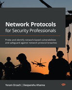
• Overclaiming – An overclaiming attack occurs when an attacker connected to the adjacent router claims that the best routing path to reach the other end of the network is provided by the attacker’s claim router, which is not true in the real-time scenario, or if the attacker’s advertisement is not authorized to accept in the network. Let’s explore this using the following figure:

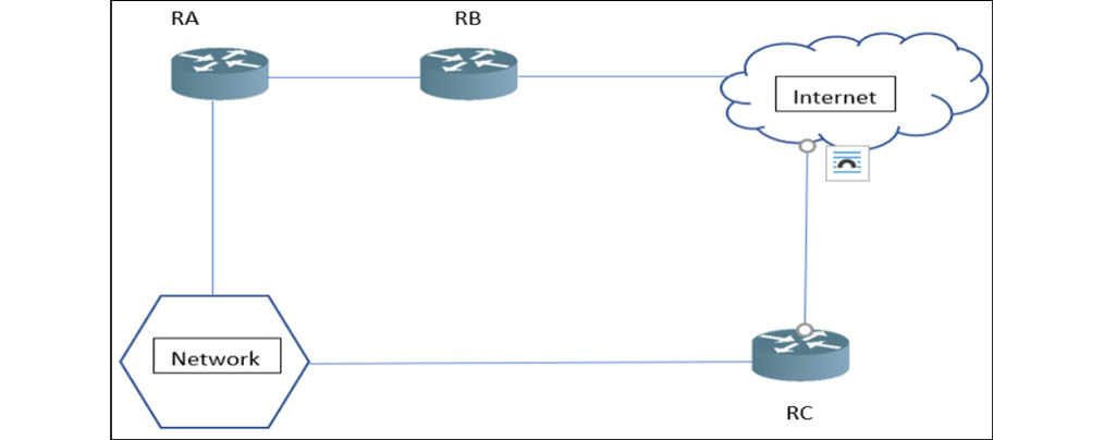
Figure 12.8 – Overclaiming

As shown in Figure 12.8, router A (RA) is connected to the internet via router B (RB) – router C (RC) is connected to the internet and the internal network the same way as RA. Now, let’s assume that in the actual scenario, RA can advertise its link to the internet through RB, and RC is authorized to advertise the links to the network. As per this scenario, RA is not authorized to advertise any link to the network, meaning that RA cannot control the links to the network, but still has a connecting link to it.

Let’s assume RA is an attacker’s router, which means the attacker is controlling the complete link states, the protocol information such as router IDs, link-state IDs, and the advertising router. Now, RA will advertise the links with fake routing, claiming that the shortest path to reach the network is through RA to RB and the internet. Once RB accepts and modifies the routing table and authorizes the traffic flow, the complete network traffic flow will start flowing through the RA, and the attacker will be able to control the traffic flow.

Now, two things could happen – either based on authorization, the traffic to the network will start flowing through RA, or the traffic will never reach the destination. But in either case, RA will be able to control the network traffic.

So, now we have understood the basics of overclaiming, let’s move on to another concept – disclaiming or misclaiming.

• Misclaiming – A misclaiming attack occurs when the attacker’s router is given some authorizations in the network and using those authorizations, the attacker starts sending the fake routing information, but that authorization is not the actual or intended authorization that was provided by the network administrator.

Let’s understand this with the help of an example, as shown in the following screenshot:

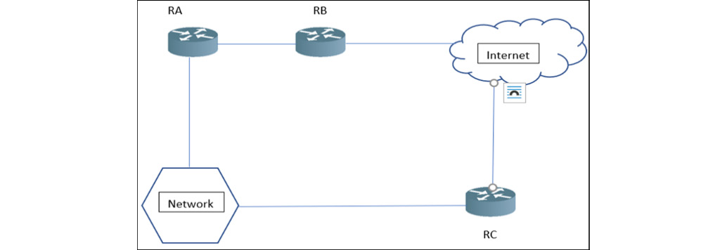
Figure 12.9 – Misclaiming

As shown in Figure 12.9, let’s suppose RA has authorized some rights in the network but not full control over the network. RA starts sending fake LSA messages to the whole network through RB. Once the fake routing LSAs are accepted, RA will be able to control the network traffic.

Now, we have understood the types of falsification with examples. Let’s look at how we can exploit this with a real-world example, as shown in the following screenshot:

Figure 12.10 – OSPF’s new integration

As shown in Figure 12.10, let’s suppose there is an integration of a new server segment in the network, and to integrate the routing, there is a new router, RC, being introduced in the network with OSPF routing.

Now, as per the default behavior of the routers, RC, to build trust with other routers in the network, will start sending the LSA with routing information – say, a 10.1.1.1/24 integration – to other routers. The other connecting routers will start updating their corresponding routing tables without checking the integrity of the routing information.

Let’s assume there is an attacker with a fake router who is also part of this network, is in MITM mode, and will also receive this information. Now, as soon as the attacker’s router receives this information, the attacker also sends a fake LSA packet in the network that the 10.1.1.1/24 network no longer supports, and the new subnet would be 192.168.1.1/24.

As soon as the other routers receive this fake LSA, they will also start updating their routing table information to build trust with the new integrated router and network. Once the routing tables are updated, the attacker will start getting traffic from the other connecting devices for the newly integrated network.

So, this is the falsification of OSPF routing by sending fake LSAs. Now we have understood these routing protocol attacks, let’s look at some other routing protocol attacks

DDOS, mistreating, and attacks on the control plane

Now, before diving deeper into the attack phase, let’s understand some of the networking basics first to define Distributed Denial-of-Service (DDOS) on control planes.

Planes

Planes in networking are simply defined as the dimensions to define how the data packet will be transmitted from the source to the destination and handled during data transmission, as well as the methods of monitoring the data transmission.

Now, these planes, in networking terminology, are divided into three categories:

• The control plane
• The data plane
• The management plane

The control plane

The control plane decides how to forward the data, which means how the data will be transferred from source to destination. The process of creating the routing table in which the routers store the network paths is part of the control plane.

The data plane

Now, once the control plane decides on the data transference, the data plane will be responsible for the transfer of data packets. The data plane is also known as the forwarding plane.

The management plane

The management plane is where the engineers configure and monitor the network devices. The management plane runs on the same processor as the control plane.

So, now we have understood the network planes, let’s look at attacks on the control plane.

DOS and DDOS

A Denial-of-Service (DOS) attack is an attempt to send many packets that will cut off the connection between the users and the network devices by increasing the load on the network or utilizing the machine’s resources. In this case, users won’t be able to access anything in the network.

Now, DDOS, on the other hand, performs the same attack but in a distributed way. A lot of BOTs will send a huge quantity of packets to utilize all the resources, which will eventually down the device and the users in the network won’t be able to access it.

Now, in the case of a control plane DDOS attack, the attackers would send a huge quantity of control packets to the device’s control plane, which would result in exhaustion and an excessive load on the router that disrupts the network communications.

Reflection attacks

A reflection attack on the control plane is another type of DOS attack that is typically different from the original DOS or DDOS attack. The reflection attack is performed in two main phases:

• Probing phase – In this phase, the attacker will first send the timing packets, test packets, and data plane packets. These packets will help the attacker to learn about the configurations of the applications of the control plane that are involved in the data plane.
• Triggering phase – Now, once the attacker gains an ample amount of information from the probing phase, they will then craft patterns for the spoofed packets to trigger the update messages in a very small time, which will cause network traffic disruptions and in some cases, the whole network can be paralyzed.

So, now we have learned about the various attacks on the control plane, let’s look at some of the attacks on the management plane.

Important Note

Performing DOS or DDOS attacks in the real-world network should be avoided, as it could bring down the whole network – losing one router or switch connection in the network can result in losing the entire network connection. Hence, demonstrating DOS or DDOS attacks is not possible for this section.

Routing table poisoning and attacks on the management plane

Routing tables are defined as the set of rules and information presented in a tabular format that determine the route of the traffic in the network. The routing table is the most important part of any routing protocol, as it represents the configuration of the routers concerning the IP addresses and is directly connected to neighboring routers.

The routing table usually consists of the destination IP address, subnet mask, and interface. This is shown as follows:

Destination Address	Subnet Mask	Interface
192.168.1.0/24	255.255.255.0	FastEthernet0/0
192.168.2.0/24	255.255.255.0	FasthEthernet0/1
Default		FastEthernet0/1

The default gateway corresponding entry to the destination address in the routing table is always 0.0.0.0 and the subnet mask is always set to 255.255.255.255.

Now, as we all know, the routing packet contains complete information about the source and the destination address. This information helps to build a proper routing table so that the routing protocol can decide the best path, as we have already seen with the OSPF protocol, and after choosing the best and shortest path, this information is also stored in the routing table.

Hence, while sending the packets from any source to the destination, the routing table will instruct the device to send packets to the next hop. The following entries are stored with every single entry in the routing table:

• Network ID – The destination address that corresponds to the route information
• Subnet Mask – The mask corresponding to the network destination address
• Next hop – The closest adjacent connecting device to which the packet will be routed
• Interface – The outgoing port from which the packet will out and reach the destination
• Metric – The minimum number of hops or routers the packet will cross to reach the destination address

So, let’s now see how this routing table looks in a router using a packet tracer.

Figure 12.11 – A routing table

As shown in Figure 12.11, the show IP route command is used to showcase the routing table information.

Let’s look at the directly connected devices, as shown in the following screenshot:

Figure 12.12 – The connected devices

As shown in Figure 12.12, the show ip route connected command shows the next hops directly connected to Router0, to which the packet will be transferred.

Now, before exploring routing table poisoning, let’s understand the issue with the Distance Vector Routing (DVR) protocol first.

The main problem with DVR is that if any router fails, the other routers will take some time to be notified about the failure, and in the meantime, the other routers will start sending the data packets, which will eventually create an infinite loop. Let’s understand this with the help of an example:

Figure 12.13 – Router failover

As shown in Figure 12.13, there are three connected routers (R0 -> R1 -> R2). Now, let’s take an example here – from R1 to R2, the total cost of a packet is 1, and from R0 to R2, it is 2.

After some time, R2 goes down, and the connection between R1 and R2 is disconnected. Now, once R1 learns about the failure, it will automatically remove the path from its table. But before sending an update to R0, R1 receives an update from R0. Now, R1 will send back an update that the total cost to reach R2 will be 3, and then once R0 receives an update, it will send the next packet with a cost of 4, and the loop will continue. This is called the Count to Infinity problem, in which the routers keep on sending false information about the cost and paths to each other in a never-ending loop.

This problem has two solutions, as listed:

• Split horizon – With this technique, if any router fails, the packet-receiving router will not send any information back to the sender router. Therefore, if R2 fails and R1 receives an update from R0, R1 will not advertise any data to R0, and hence, the loop can be avoided.
• Routing poison – With this technique, if any router in the network fails, the connecting neighbor router will start sending negative information about the failure with a very special metric value called infinity, which will inform the other routers that there is a connection failure at a certain end. Every routing protocol has its definitive infinity value – for example, with RIP, it is 16.

Now, once the routers receive the infinity value, all the routers accept this information and modify the routing table. But the main issue with route poisoning is that the number of announcements increases, which can flood the environment.

Now we have understood the routing table, its issues, and why routing poison was introduced. Now, think from an attacker’s perspective that if an attacker starts sending fake announcements in the network and can modify the routing tables, it eventually causes the network to malfunction or be completely compromised.

Now, we can create the packets and route for fake routing table entries – there is an automated tool for this written by Frederico. You can find it here: https://gitlab.com/fredericopissarra/t50/-/releases.

The following figure shows the automated tool attack:

Figure 12.14 – Routing table poisoning

As shown in Figure 12.14, 1,000 fake packets are flooded and will poison the routing tables with fake entries.

Now, similar types of attacks can be performed on the management plane, in which an attacker attacks and controls the switches:

• CAM table poisoning – A Content Addressable Memory (CAM) table is created by switches in the network to store the information about the MAC addresses, along with their corresponding VLAN parameters. The following screenshot shows the CAM table entries in the switch:

Figure 12.15 – A CAM table

As shown in Figure 12.15, the show mac-address table presents the CAM table entries in the switch.

Now, an attacker can flood this CAM table with fake entries using the macof tool, which is pre-installed in Kali Linux. The following screenshot shows the macof tool:

Figure 12.16 – CAM table poisoning

As shown in Figure 12.16, 10 entries in the MAC table were sent to poison the MAC table of the switch connected at eth0.

• Address Resolution Protocol (ARP) – We showcased ARP poisoning in detail in Chapter 8, Network Traffic Analysis and Eavesdropping, in the ARP spoofing attacks section. In this chapter, we'll look at some other ways to attack switches in layer 2.
• Protocol-based attacks – There are also attacks on Simple Network Management Protocol (SNMP) or Secured Shell (SSH) protocols that are not covered in this chapter, but please feel free to explore this as well.

Now that we have seen the attacks on switches and routers, let us look at the security configurations for routers.

Traffic generation and attacks on the data plane

Nowadays, building networks is much more complex than it used to be. Performing network-related tests is a much more difficult task for network administrators, especially in terms of bandwidth testing, any glitch that has caused the intermediate connecting network devices to disconnect from the network, or tracing the packet loss between the host and the server.

Therefore, packet generation plays a vital role in troubleshooting network issues. Hence, packet generation is a type of traffic generation that defines the flow of the packets and data sources between the client and the server in a packet-switched network. For example, in the case of the web, traffic is sent in the form of web packets to be received and sent by the user’s browser.

Therefore, traffic generation defines the flow of certain traffic between the sender and the receiver in a certain format and network, such as cellular networks or computer networks.

Now, for this book and chapter, we will focus on computer networks, but please feel free to explore cellular traffic as well.

To analyze the traffic performance in real time, there are numerous tools present on the internet such as Bwping or iperf. But as per my experience, network administrators generally prefer using iperf, because it is very user-friendly, comes with multiple options, is compatible with Windows and Linux (both flavors), gives accurate details, and most importantly, can generate both TCP and UDP packets.

So, let us analyze the traffic bandwidth by generating a certain number of packets between the client and server.

Now, to generate the traffic between two hosts, we need to create a server listener at one end, as shown in the following screenshot:

Figure 12.17 – Opening the iperf listener

As shown in Figure 12.17, a listener is a setup at the one end of the network. Now, let’s set up a client on another end of the network, as shown in the following screenshot:

`

Figure 12.18 – iperf connected with the listener

As shown in Figure 12.18, the machine on another end is connected to the machine with the listener open, and as we can see, there is an exchange of traffic at a bandwidth rate of 35.4 Gbits/sec.

We can monitor the same thing in the system monitor window, where the memory utilization graph peaks during the exchange of traffic or traffic generation:

Figure 12.19 – The peak when the traffic exchange started

As shown in Figure 12.19, before the client connected to the listener machine, the traffic exchange was normal and CPU utilization was lower, but as soon as the client is connected to the server, there is an exchange of traffic, causing the CPU utilization to immediately go up and manifesting as a visible peak in the network.

Attacks on the data plane

Now, attacks on the data plane are similar to the types of attacks we have seen performed on the management plane, but the nature of the attacks will be completely different.

So, as we know, the data plane is the carrier of the data packets – hence, the following are the levels of attacks that can be performed here:

• Eavesdropping – Eavesdropping is a mechanism by which an attacker monitors and modifies the ongoing traffic between the two nodes. This attack generally depends upon the type of the packets but generally, attackers perform an ARP relay to sniff the complete traffic. We discussed this in Chapter 8, Network Traffic Analysis and Eavesdropping, in depth.
• DOS – Another major attack that is very common on the data plane is a DOS attack, mainly performed for two reasons:
  • Breaking the complete connection between both the communicating parties
  • Sending malformed traffic to redirect the requests generally performed during wireless attacks

So, let’s look at a DOS attack on the data plane:

Figure 12.20 – hping3 flooding the service running at port 80

As shown in Figure 12.20, the attack is started at port 80 on a server running at 192.168.64.130. After some time, the server wasn’t reachable:

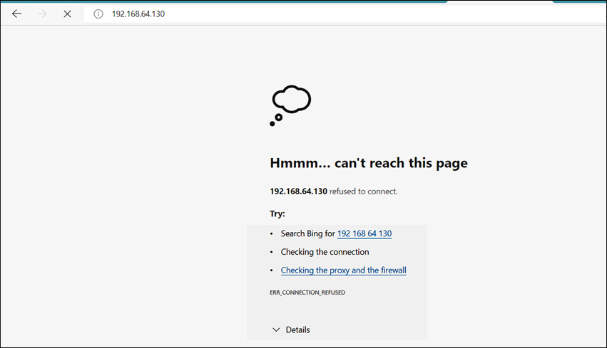
Figure 12.21 – The server is down

As shown in Figure 12.21, the service is down. Now, we have seen multiple attacks on routers and routing protocols, let’s look at the security configurations at the router’s end.

How to configure your routers to protect

Now we have seen various types of attacks on routers, let’s look at the high-level security best practices that can be applied to the routers to protect against various levels of attacks:

• The Authentication, Authorization, Accounting (AAA) framework – The AAA framework provides a centralized approach that provides mechanisms for the authentication of the user’s management sessions. The AAA framework also provides a secure configuration to limit the number of commands that will be enabled by the administrators and will also help to log all the commands enabled by the users.
• A secure management plane configuration – As defined earlier, the management plane is responsible for monitoring and managing the device and network operations on which it is deployed. The management plane should be configured securely, as all the data from the control plane directly affects the operations of the management plant. The following protocols should be configured securely at the management plane:
  • SNMP
  • SSH
  • Terminal Access Controller Access Control System (TACACS+)
  • Radius
  • Telnet
  • File Transfer Protocol (FTP)
  • Network Time Protocol (NTP)
• Centralized monitoring and security operations – Monitoring should be enabled among all the network devices. It will monitor the complete inbound or outbound traffic, which will prevent unauthorized access alerts or attack alerts. This can be achieved by SIEM monitoring and NetFlow.

NetFlow – A technology used by network administrators to monitor the traffic flow to and from the routers.

• Password management – Credentials play a key role in any machine that helps to authenticate the machines. Similarly, to authenticate routers, network administrators generally enable SSH for communication. Generally, during the penetration phase, the attackers can break the credentials, as administrators generally keep low-strength or common passwords such as Admin@123, which should not be used in general practice.

Hence, a strong login password should be set for SSH. In addition to this, the administrators should use a stronger encryption mechanism to authenticate the administrators at the router’s IOS config level. This can be achieved by using the enable secret command.

Another security implementation that should be carried out is the implementation of the TACACS+ or Radius password management server. This enables the authentication requests to check the access level granted to the users or groups first and then based on the permissions set, the access is granted or denied.

Network administrators should also set the lockout feature in routers. This will prevent and lock the users after three to five failure attempts:

• No Service Password-Recovery – The No Service Password-Recovery feature prevents access to modify the NVRAM and change the configuration register value.
• Centralized logging – Logging helps the administrators, as well as the security professionals, to look at the logs during network communication failures or in case of security breaches.
• Restricting idle services – During the initial implementation of routers, there will also be a lot of unrestricted services enabled. This can help attackers to exploit and gain access to routers through the SNMP, for example – attackers can not only modify the router parameters but can also change the router’s configurations. Hence, disable the unused services and restrict the essential protocols.
• Access Control Lists (ACLs) – ACLs play a vital role in an environment. These ACLs are called infrastructure ACLs. ACLs decide the network traffic flow, such as whether to restrict or allow any traffic packet from one area to another. The major example of this like traffic only allows from SSH or SNMP.

There are other types of ACLs besides infrastructure ACLs, known as VLAN ACLs (VACLs). These VACLs will enforce the traffic rules routed to and from inter-VLAN or intra-VLAN. These VACLs protect the environment using both segmentation and segregation. For example, SWIFT environments are often placed in an isolated zone, and these are separated from the whole environment using the VACLs:

• NTP – NTP is always an easy target for any attacker. Hence, NTP should be secured with NTP authentication.
• Secure protocols – Another very important factor is the configuration of secure protocols such as SSHv2, SNMPv3, and the filtering of traffic protocols such as Internet Control Message Protocol (ICMP).
• Implementation of DOS or DDOS – DOS or DDOS attacks are very common in the network. Hence, there are many solutions available given by CISCO and other entities such as Juniper to protect against DOS or DDOS attacks.

  Important Note

  These are some of the important configurations that protect against network intrusions. For the complete information, CISCO has published a complete document on secure router configurations. Please follow the link for complete information: https://www.cisco.com/c/en/us/support/docs/ip/access-lists/13608-21.html.

BGP – protocol and operation

BGP is an EGP that was introduced in 1984 as v1 to route the network packets by choosing the best routing path. Hence, BGP is also known as the dynamic routing protocol.

So, as time evolved, the internet started growing, and the network traffic eventually started putting a greater load on the communication channels. Hence, the BGP was reframed and multiple versions were introduced. The current version of BGP is v4.

Now, as we know, for routers to communicate outside of their AS, they need to have BGP configured. The local network administrator will not know which AS number they should configure under. So, to solve all the AS and BGP configuration issues, all organizations take the AS configurations from their ISP. Hence, the ISP will put the organization’s network routes under its own AS, making it a single AS to route traffic from the organization to the global internet.

So, as with OSPF, BGP also transfers the data by choosing the best path for transfer, but not in the way that OSPF parameters do. BGP works with path parameters to choose the best, such as based on the number of hops, which in networking terms, is known as the distance vector protocol. In this way, the routing protocol will calculate the number of hops between the source and destination. This is shown as follows:

Figure 12.22 – BGP distance vector calculation

As shown in Figure 12.22, the source AS, A100, sends the requests and collects the responses from both distance vectors. Now, based on distance vector calculation, BGP will choose Distance vector 2 as the best path, as it only has two AS hops to reach the destination.

Now, there is another very important concept in BGP – it’s programmed to work smartly to avoid loops horizons. This means that if the source AS receives a loop AS a number of its own, creating a loop, then it simply rejects the path and chooses the second-best path after this. Let’s understand this with the help of a diagram as follows:

Figure 12.23 – BGP distance vector calculation (loop horizon)

As shown in Figure 12.23, the first distance vector that BGP receives forms a loop, and hence, BGP will simply drop the path. So, let us now look at the BGP tables and messages.

BGP creates three tables:

• Neighbor tables – This table contains all the entries of the adjacent connecting AS.
• BGP tables – This table contains all the information about the BGP routing such as all the identified paths and prefixes.
• BGP routing – This contains information about the best path selection for data transmissions.

BGP uses four different types of messages:

• OPEN
• UPDATE
• KEEPALIVE
• NOTIFICATION

So, now we have covered the operation of BGP. Let us now look at how BGP works in real time through simulation in Packet Tracer:

Figure 12.24 – BGP configuration in packet tracer

As shown in Figure 12.24, the BGP is configured for Router1, and the same configuration is being done at Router0 and Router2. Now, once all the routers learn about each connecting node, the source can then start the data transmission.

Now, we have learned the BGP in depth. Let’s look at some of the flaws of BGP.

BGP hijacking

BGP hijacking in simple terms is defined as the rerouting of the ongoing traffic from one AS to another AS, which is completely owned by the attackers. BGP hijacking is also known as prefix, route, or IP hijacking.

Let’s understand this with a small example. Imagine every day everyone takes different routes from home in the morning to reach the same destination, which only has a single road to go and come back from it. Now, suddenly, one day, a parallel road is designed by hijackers, and as an announcement, a sign has been installed that signals that this is the shortest road to reach the destination, so everybody turns down that newly built road. After this, all of the traffic will eventually be hijacked by the attacker. Let’s frame this with a simple diagram, as shown in the following figure:

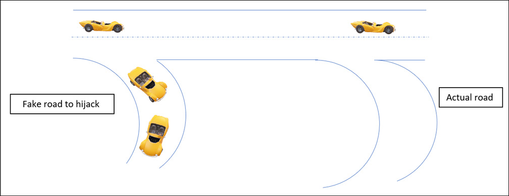
Figure 12.25 – Traffic hijacking

As shown in Figure 12.25, an attacker or a hijacker created a fake road just parallel to the other road, so now all the traffic will be rerouted to the fake road.

So, a similar idea can be applied to BGP hijacking. Now, attackers will corrupt the internet routing tables and illegitimately take over the IP addresses. To achieve this, the attackers will own a router and announce the IP addresses that are currently not assigned to the attacker’s router. This request will offer the other routers to route the traffic with the shortest path and the source router will add the router ID to the BGP routing table, which will eventually redirect the traffic to the attacker’s own IP address. The complete attack pattern is shown in the following screenshot:

Figure 12.26 – BGP hijacking

As shown in Figure 12.26, an attacker announced an IP address with the shortest route for the destination.

So, now that we have learned about BGP hijacking, let’s look at what would happen if the BGP is hijacked:

• An attacker would be able to monitor and control the complete internet traffic.
• The internet traffic could be routed to a different zone such as malicious sites.
• Spammers can use BGP hijacking to spoof legitimate IP addresses for illegitimate work.
• The attackers can increase the latency for the complete internet traffic.

There will be many other scenarios, such as hackers performing BGP hijacking in 2018 who were able to steal approximately $152,000 in the form of digital money or cryptocurrency.

Now, let’s demonstrate BGP hijacking in a real-time scenario, as shown in the following figure:

Figure 12.27 – A current BGP configuration

As shown in Figure 12.27, the current BGP configuration for the corresponding next hop in the R5 router for the 1.0.0.0 network is 9.0.6.1/9.0.7.1, and similarly for other networks as well.

Now, an attacker will create a rogue AS and fake the route information to send the traffic through the rogue AS, as shown in the following figure:

Figure 12.28 – The current BGP configuration

As shown in Figure 12.28, with a fake AS, there is a new entry to the 1.0.0.0 network with the corresponding next hop being 9.0.8.2/9.0.5.2. Now, all the traffic will be routed through these new network configurations.

Now, we understand how dangerous it would be if BGP protocol was hijacked. So, let’s understand how we can protect it.

BGP mitigation

The following methods can be used to prevent BGP hijacking:

• BGP hijacking detection – Proper monitoring of the BGP-routed traffic can help organizations to avoid BGP hijacking. This can be achieved if there is any latency being seen in the network traffic from the normal latency Time To Live (TTL).
• IP prefix filtering – The network administrators or ISPs should only declare the fixed IP addresses rather than the complete internet. This will prevent the routers to accept the fake IP address prefix declarations and also help in preventing unintentional route hijacking.
• BGPSec – Implement BGPSec, which will implement another layer of security at the BGP protocol.

Summary

In this chapter, we learned in depth about how types of IGP and EGP such as OSPF, RIP, BGP, and IS-IS and their corresponding analyses using various packet sniffers and GUI-based network simulations such as Packet Tracer and GNS3. Then, we learned about the BGP. Apart from routing protocols, we performed various practical demonstrations of attacks such as routing table poisoning and BGP hijacking and also learned about the various mitigation techniques of routing protocols and how we can securely configure the routers.

Now, in the next chapter, we will learn about a very important protocol from the attacker’s point of view, which is Domain Name Service (DNS), its behavior analysis using sniffers, and the practical demonstration of various real-time attacks on DNS.

Questions

1. What is the full form of OSPF?
   1. Open Shortest Path First
   2. Open Small Path First
   3. Open Shortest Payload First
   4. None of the above
2. What is the full form of BGP?
   1. Bi Gate Protocol
   2. Border Gateway Protocol
   3. Border Gate Protocol
   4. None of the above
3. What does the EGP include?
   1. OSPF
   2. RIP
   3. BGP
   4. All of the above
4. What does the IGP include?
   1. OSPF
   2. RIP
   3. Static
   4. Both A and B
5. How is the Count to Infinity problem resolved?
   1. BGPSec
   2. Split horizon
   3. Gateway to last resort
   4. None of the above
6. What is BGPSec protection against?
   1. BGP hijacking
   2. Routing loops
   3. Hop counts
   4. All the above
7. What is the tool used for routing table poisoning?
   1. macof
   2. Kali
   3. T50
   4. All of the above