Chapter 10
Iteratively Decoded Variable-Length Space–Time Coded Modulation: Code Construction and Convergence Analysis1
10.1 Introduction
In this chapter an Iteratively Decoded Variable-Length Space–Time Coded Modulation (VL-STCM-ID) scheme capable of simultaneously providing both coding and iteration gain as well as multiplexing and diversity gain is investigated. Non-binary unity-rate precoders are employed in order to assist the iterative decoding of the VL-STCM-ID scheme. The discrete-valued source symbols are first encoded into variable-length codewords that are spread to both the spatial and the temporal domains. Then the variable-length codewords are interleaved and fed to the precoded modulator. More explicitly, the proposed VL-STCM-ID arrangement is a jointly designed iteratively decoded scheme combining source coding, channel coding and modulation as well as spatial diversity/multiplexing. We demonstrate that, as expected, the higher the source correlation, the higher the achievable performance gain of the scheme becomes. Furthermore, the performance of the VL-STCM-ID scheme is about 14 dB better than that of the Fixed-Length STCM (FL-STCM) benchmark at a source symbol error ratio of 10−4.
To elaborate a little further, recall from Chapter 1 that Shannon’s separation theorem stated that source coding and channel coding are best carried out in isolation [133]. However, this theorem was formulated in the context of potentially infinite-delay, lossless entropy coding and infinite-block-length channel coding. In practice, real-time wireless audio and video communications systems do not meet these ideal hypotheses. Explicitly, the source-encoded symbols often remain correlated, despite the lossy source encoder’s efforts to remove all redundancy. Furthermore, they exhibit unequal error sensitivity. In these circumstances, it is often more efficient to use jointly designed source and channel encoders.
The wireless communication systems of future generations will be required to provide reliable transmissions at high data rates in order to offer a variety of multimedia services. Space–time coding schemes, which employ multiple transmitters and receivers, are among the most efficient techniques designed for providing high data rates by exploiting the high channel capacity potential of Multiple-Input Multiple-Output (MIMO) channels [314, 315]. More explicitly, the Bell Labs LAyered Space–Time architecture (BLAST) [316] was designed for providing full-spatial-multiplexing gain, while Space–Time Trellis Codes (STTCs) [317] were designed for providing the maximum attainable spatial-diversity gain.
As a further advance, in this chapter we investigate a jointly designed source coding and Space–Time Coded Modulation (STCM) scheme, where two-dimensional (2D) Variable-Length Codes (VLCs) are transmitted by exploiting both the spatial and the temporal domains. More specifically, the number of activated transmit antennas equals the number of modulated symbols in the corresponding VLC codeword in the spatial domain, where each VLC codeword is transmitted during a single symbol period. Hence, the transmission frame length is determined by the fixed number of source symbols, and therefore the proposed Variable-Length STCM (VL-STCM) scheme does not exhibit synchronization problems and does not require the transmission of side information for synchronization. Additionally, the associated source symbol correlation is exploited in order to achieve an increased product distance, hence resulting in an increased coding gain. Furthermore, the VL-STCM scheme advocated is capable of providing both multiplexing and diversity gains with the aid of multiple transmit antennas. Practical applications of the proposed scheme are related to the transmission of VLC-based MPEG-2-, 3-and 4-encoded video and audio sequences, for example. It is also possible to simply pack binary computer data into VLC-encoded symbols for the sake of removing any correlation amongst the symbols and for their near-capacity transmission.
Relevant work on the joint design of source coding and space–time coding can be found in [318] and [319], where the performance measure is based on the end-to-end analog source distortion. However, in this chapter we assume the presence of a discrete source, where the potentially analog source was quantized/discretized, before it was input to our VL-STCM encoder. Our objective is thus to minimize the error probability of the discrete source symbols. Furthermore, joint detection of conventional One-Dimensional (1D) VLC and STCM has been shown to approach the channel capacity in [320], although the related VLC schemes have to convey explicit side information regarding the total number of VLC-encoded bits or symbols per transmission frame.
On the other hand, it was shown in [321] that a binary Unity-Rate Code (URC) or precoder can be beneficially concatenated with Trellis-Coded Modulation (TCM) [322] for the sake of invoking iterative detection, and hence for attaining iteration gains. Since VLSTCM also belongs to the TCM family, we further develop the VL-STCM scheme for the sake of attaining additional iteration gains by introducing a novel non-binary URC between the variable-length space–time encoder and the modulator. The Iterative Decoding (ID) VLSTCM (VL-STCM-ID) scheme achieves a significant coding/iteration gain over both the non-iterative VL-STCM scheme and the Fixed-Length STCM (FL-STCM) benchmark.
The rest of the chapter is organized as follows. The overview of the space–time coding technique advocated is given in Section 10.2 and the 2D VLC design is outlined in Section 10.3. The description of the proposed VL-STCM and VL-STCM-ID schemes is presented in Sections 10.4 and 10.5 respectively. The convergence of the VL-STCM-ID scheme is analyzed in Section 10.6. In Section 10.7 the performance of the proposed schemes is discussed. Then the VL-STCM is combined with a higher-order modulation scheme in Section 10.8. Finally our conclusions are offered in Section 10.9.
10.2 Space–Time Coding Overview
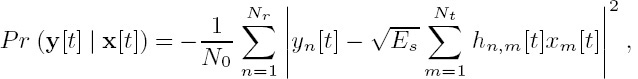
Let us consider a MIMO system employing Nt transmit antennas and Nr receive antennas. The signal to be transmitted from transmit antenna m, 1 ≤ m ≤ Nt, at the discrete time index t is denoted as xm [t]. The signal received at antenna n, 1 ≤ n ≤ Nr, and at time instant t can be modeled as

where Es is the average energy of the signal constellation and hn,m[t] denotes the flat-fading channel coefficients between transmit antenna m and receive antenna n at time instant t, while wn[t] is the Additive White Gaussian Noise (AWGN) having zero mean and a variance of N0/2 per dimension. The amplitude of the modulation constellation points is scaled by a factor of ![]() so that the average energy of the constellation points becomes unity and the expected Signal-to-Noise Ratio (SNR) per receive antenna is given by γ = NtEs/N0 [323]. Let us denote the transmission frame length as T symbol periods and define the space–time encoded codewords over T symbol periods as an (Nt × T)-dimensional matrix C formed as
so that the average energy of the constellation points becomes unity and the expected Signal-to-Noise Ratio (SNR) per receive antenna is given by γ = NtEs/N0 [323]. Let us denote the transmission frame length as T symbol periods and define the space–time encoded codewords over T symbol periods as an (Nt × T)-dimensional matrix C formed as

where the elements of the tth column c[t]=[c1[t] c2[t] · · · cNt[t]]T are the space–time symbols transmitted at time instant t and the elements in the mth row cm = [cm [1] cm [2] · · · cm [T]] are the space–time symbols transmitted from antenna m. The signal transmitted at time instant t from antenna m, which is denoted as xm[t] in Equation (10.1), is the modulated space–time symbol given by xm[t]= f(cm[t]) where f(.) is the modulator’s mapping function. The Pair-Wise Error Probability (PWEP) of erroneously detecting E instead of C is upper bounded at high SNRs by [317, 324] where EH is referred to as the effective Hamming distance, which quantifies the transmitter-diversity order, and EP is termed the effective product distance [317], which quantifies the coding advantage of a space–time code.

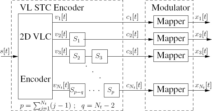
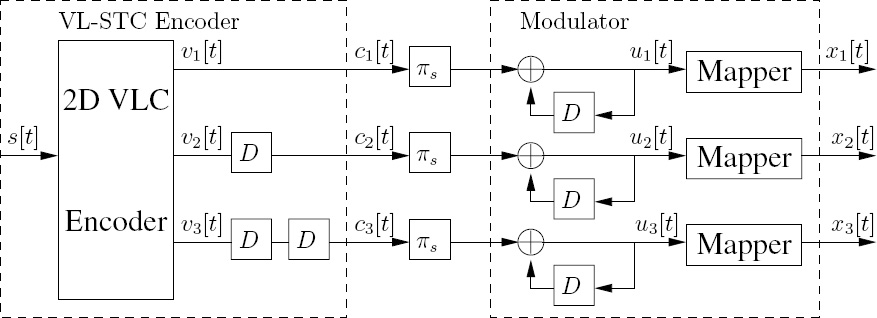
Figure 10.1: Block diagram of the VL-STCM transmitter. IEEE [271] Ng et al.2007.
It was shown in [325] that a full-spatial-diversity STTC scheme having the minimum decoding complexity can be systematically designed based on two steps. The first step is to design a block code, while the second step is to transmit the block code diagonally across the space–time grid. The mechanism of the diagonal transmission across the space–time grid will be exemplified in Section 10.4 in the context of Figure 10.1. The Hamming distance and the product distance of a block code can be preserved when the block code is transmitted diagonally across the space–time grid. Hence, a full-spatial-diversity STTC scheme can be realized, when the Hamming distance of the block code used by the STTC scheme equals the number of transmitters. Based on the same principle, a joint source-coding and STTC scheme can be systematically constructed by first designing a 2D VLC and then transmitting the 2D VLC diagonally across the space–time grid. As mentioned above [325], this allows us to achieve a transmitter-diversity order2, which is identical to the Hamming distance of the 2D VLC plus a coding advantage quantified by the product distance of the 2D VLC, as well as a multiplexing gain, provided that the number of possible source symbols Ns is higher than the number of modulation levels M.
Let us now commence our detailed discourse on the proposed VL-STCM-ID scheme in the following sections.
10.3 Two-Dimensional VLC Design
Consider as an example a source having Ns = 8 possible discrete values, and let the lth value be represented by a symbol sl = l for l ∈ {1, 2, ..., Ns}. Let us consider a source where the symbols emitted are independent of each other, but the symbol probability distribution is not uniform, and is given by
and ![]() Hence, the source symbol s1 has the highest occurrence probability of P(s1) = 0.4068, and the source symbol s8 has the lowest occurrence probability of P(s8) = 0.0114. Note that a source is correlated when its entropy rate
Hence, the source symbol s1 has the highest occurrence probability of P(s1) = 0.4068, and the source symbol s8 has the lowest occurrence probability of P(s8) = 0.0114. Note that a source is correlated when its entropy rate ![]() (s) is smaller than log2(Ns) [326]. For the independent source considered, the source entropy rate equals the source entropy H(s), which is given by
(s) is smaller than log2(Ns) [326]. For the independent source considered, the source entropy rate equals the source entropy H(s), which is given by ![]() (s) = H(s) =
(s) = H(s) = ![]() = 2.302 bit. Since
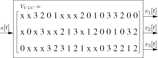
= 2.302 bit. Since ![]() (s) < log2(Ns), the source considered is a correlated source, where the higher the source correlation the smaller the source entropy rate. Let us now consider a 2D VLC codeword matrix, VVLC, which encodes these Ns = 8 possible source symbols using Nt = 3 transmit antennas and BPSK modulation as follows:
(s) < log2(Ns), the source considered is a correlated source, where the higher the source correlation the smaller the source entropy rate. Let us now consider a 2D VLC codeword matrix, VVLC, which encodes these Ns = 8 possible source symbols using Nt = 3 transmit antennas and BPSK modulation as follows:

where each column of the (3 × 8)-dimensional matrix VVLC corresponds to the specific VLC codeword conveying a particular source symbol, and the elements in the matrix denoted as ‘0’ and ‘1’ represent the BPSK symbols to be transmitted by the Nt = 3 transmit antennas, while ‘x’ represents ‘no transmission.’ ‘No transmission’ implies that the corresponding transmit antenna sends no signal. Let the lth source symbol sl be encoded using the lth column of the VVLC matrix seen in Equation (10.5). Hence, the source symbol s1 is encoded into an Nt-element codeword using the first column of VVLC in Equation (10.5), namely [x x 0]T, where the first and second transmit antennas are in the ‘no transmission’ mode, while the third antenna transmits an ‘active’ symbol represented by the binary value ‘0’. If L(sl) is the number of ‘active’ symbols in the VLC codeword assigned to source symbol sl, then we may define the average codeword length of the 2D VLC as
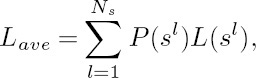
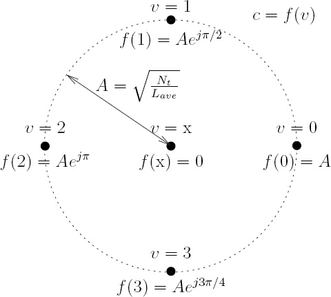
where we have Lave = 1.233 bits/VLC codeword for this system according to Equations (10.4) and (10.5). The corresponding BPSK signal mapper is characterized in Figure 10.2, where the ‘no transmission’ symbol is actually represented by the origin of the Euclidean space, i.e. we have f(x) = 0, where f(.) is the mapping function. Since the ‘no transmission’ symbol is a zero-energy symbol, the amount of energy saving can be computed from
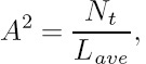
where we have A2 = 3/1.233 = 2.433, which is equivalent to 20 log(A) = 3.86 dB. Hence, more transmitted energy is saved, when there are more ‘no transmission’ symbols in a VLC codeword. Therefore, the columns of the matrix VVLC in Equation (10.5), which are the VLC codewords, and the source symbols are specifically arranged so that the more frequently occurring source symbols are assigned to VLC codewords having more ‘no transmission’ components, in order to save transmit energy. The energy saved is then reallocated to the ‘active’ symbols for the sake of increasing their minimum Euclidean distance, as shown in Figure 10.2.
Figure 10.2: The signal mapper of the VL-STCM. © IEEE [271] Ng et al. 2007.

Let us define the Hamming distance EH min as the number of different symbol positions of all the columns in the 2D VLC codeword matrix. Hence, we have EH min = 2 for the 2D VLC codeword matrix in Equation (10.5). We further define the minimum product distance EP min as
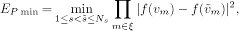
where ξ represents the set of VLC codeword component indices m satisfying the condition of ![]() for 1 ≤ m ≤ Nt and the VLC codeword v = [v1 v2 ... vNt]T is defined in Figure 10.1 and Equation (10.5). The two VLC codewords conveying the source symbols s and
for 1 ≤ m ≤ Nt and the VLC codeword v = [v1 v2 ... vNt]T is defined in Figure 10.1 and Equation (10.5). The two VLC codewords conveying the source symbols s and ![]() are represented as [v1 ...vNt]T and
are represented as [v1 ...vNt]T and ![]() respectively, in Equation (10.8). We have EP min = 5.92based on Equation (10.5) and the signal mapper of Figure 10.2. Note that the mapper function f(.) used in Equation (10.8) and portrayed in Figure 10.2 depends on the amount of energy saving. The amount of energy saving is given by Equation (10.7), where the numerator Nt is fixed and the denominator Lave is given by Equation (10.6). As in the conventional 1D VLC, the higher the source correlation, the lower the average codeword length Lave of the 2D VLC. A higher energy saving can be attained when the source is more correlated, due to a reduced average codeword length Lave. In other words, the source correlation is converted into an increased minimum product distance, resulting in an increased coding gain when the source is more correlated. By contrast, the conventional 1D VLC exploits the source correlation in order to attain an increased compression ratio.
respectively, in Equation (10.8). We have EP min = 5.92based on Equation (10.5) and the signal mapper of Figure 10.2. Note that the mapper function f(.) used in Equation (10.8) and portrayed in Figure 10.2 depends on the amount of energy saving. The amount of energy saving is given by Equation (10.7), where the numerator Nt is fixed and the denominator Lave is given by Equation (10.6). As in the conventional 1D VLC, the higher the source correlation, the lower the average codeword length Lave of the 2D VLC. A higher energy saving can be attained when the source is more correlated, due to a reduced average codeword length Lave. In other words, the source correlation is converted into an increased minimum product distance, resulting in an increased coding gain when the source is more correlated. By contrast, the conventional 1D VLC exploits the source correlation in order to attain an increased compression ratio.
The design of the 2D VLC scheme is summarized in Algorithm 10.1.
Note that the search-space of Step 1 can be significantly reduced with the aid of the branch-and-bound algorithm of [327], where both EH min and EP min are used during the bounding operation. By contrast, the code search in [320, 325] also employs the branch-and-bound algorithm, but uses only EP min in the bounding operation. The 2D VLC matrix seen in Equation (10.5) was designed based on the above three steps. When Nt = 3 transmit antennas are employed for transmitting the Nt-element 2D VLC codewords denoted as ![]() in Figure 10.1, we achieve a transmitter-diversity order of EH min = 2, a coding gain quantified by EP min = 5.92 and a spatial multiplexing gain quantified by log2(Ns/M) = 2, where M = 2 is the number of modulation levels of the original BPSK modulation and Ns = 8 is the number of source symbols. The throughput of the scheme is given by η = log2(Ns) = 3 bit/s/Hz and the Signal-to-Noise Ratio (SNR) per bit is given by Eb/N0 = γ/η, where γ is the SNR per receive antenna.
in Figure 10.1, we achieve a transmitter-diversity order of EH min = 2, a coding gain quantified by EP min = 5.92 and a spatial multiplexing gain quantified by log2(Ns/M) = 2, where M = 2 is the number of modulation levels of the original BPSK modulation and Ns = 8 is the number of source symbols. The throughput of the scheme is given by η = log2(Ns) = 3 bit/s/Hz and the Signal-to-Noise Ratio (SNR) per bit is given by Eb/N0 = γ/η, where γ is the SNR per receive antenna.
Based on the above design principles, a range of 2D VLCs can be created for M-ary PSK modulation for M > 2, where the origin of the Euclidean space represents the ‘no transmission’ symbol.
|
1. Search for all possible VLC codeword matrices that have the maximum achievable minimum Hamming distance EH min and product distance EP min values, for each pair of the VLC codewords at a given Ns and Nt combination. Note that attaining a higher EH min is given more weight than EP min, since EH min is more dominant in the PWEP of Equation (10.3). 2. Rearrange the columns of the VLC codeword matrices in descending orders according to the number of ‘no transmission’ components. Assign the source symbols to the columns of the VLC codeword matrix, in descending orders according to the symbol probabilities. 3. Find the VLC codeword matrix that gives the shortest average codeword length, with the aid of Equation (10.6). 4. Assign the more frequently occurring source symbols to the VLC codewords having more ‘no transmission’ components, in the interest of saving transmission power. |
10.4 VL-STCM Scheme
The block diagram of the VL-STCM transmitter is illustrated in Figure 10.1, which can be represented by two fundamental blocks, namely the Variable-Length Space–Time Code (VL-STC) encoder and the modulator. As seen in Figure 10.1, a VLC codeword v[t]= [v1[t]v2[t] · · · vNt[t]]T is assigned to each of the source symbols s[t] generated by the source at time instant t, where we have s[t] ∈ {1, ..., Ns} and Ns denotes the number of possible source symbols. Each of the VLC codewords v[t] seen in Figure 10.1 corresponds to one of the columns in the VLC matrix of Equation (10.5). Hence, the component vm[t] of the VLC codeword is represented by a symbol seen in the VLC matrix of Equation (10.5). As portrayed in Figure 10.1, the VLC codeword v[t]is transmitted diagonally across the space–time grid with the aid of appropriate-length shift registers, denoted as Sk in Figure 10.1, where we have ![]() As we can see from Figure 10.1, the codeword v[t]=[v1[t] v2[t] · · · vNt[t]]T is transmitted using Nt transmit antennas, where the mth element of each VLC codeword, for 1 ≤ m ≤ Nt, is delayed by (m − 1) shift register cells before it is transmitted through the mth transmit antenna. Hence, the Nt components of each VLC codeword are transmitted on a diagonal of the space–time codeword matrix of Equation (10.2). Since the VLC codewords are encoded diagonally, the space–time coded symbol cm[t] transmitted by the mth antenna, 1 ≤ m≤ Nt, at a particular time-instant t is given by cm[t] = vm[t−m+1]. Thus, for this specific case each element of the space–time codeword matrix of Equation (10.2) is given by cm[t] = vm[t−m + 1], while the transmitted signal is given by
As we can see from Figure 10.1, the codeword v[t]=[v1[t] v2[t] · · · vNt[t]]T is transmitted using Nt transmit antennas, where the mth element of each VLC codeword, for 1 ≤ m ≤ Nt, is delayed by (m − 1) shift register cells before it is transmitted through the mth transmit antenna. Hence, the Nt components of each VLC codeword are transmitted on a diagonal of the space–time codeword matrix of Equation (10.2). Since the VLC codewords are encoded diagonally, the space–time coded symbol cm[t] transmitted by the mth antenna, 1 ≤ m≤ Nt, at a particular time-instant t is given by cm[t] = vm[t−m+1]. Thus, for this specific case each element of the space–time codeword matrix of Equation (10.2) is given by cm[t] = vm[t−m + 1], while the transmitted signal is given by
for 1 ≤ m ≤ Nt. Note that originally there were only Ns = 8 legitimate 2D-VLC codewords in Equation (10.5). However, after these VLC codewords are diagonally mapped across the space–time grid using the shift registers shown in Figure 10.1, there is a total of ![]() Nt = 33 = 27 legitimate space–time codewords3, where
Nt = 33 = 27 legitimate space–time codewords3, where ![]() is the number of possible symbols in each position of the 2D VLC codewords. Note, however, that the number of legitimate space–time codewords may become lower than
is the number of possible symbols in each position of the 2D VLC codewords. Note, however, that the number of legitimate space–time codewords may become lower than ![]() Nt when a different 2D VLC codeword matrix is employed.
Nt when a different 2D VLC codeword matrix is employed.
Table 10.1: The space–time codeword table. ©IEEE [271] Ng et al.2007.
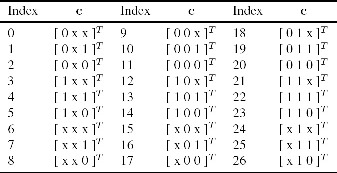
The corresponding trellis diagram of the proposed VL-STC encoder is depicted in Figure 10.3. The Nt = 3-element space–time codeword seen in Figure 10.1 is given by c = [c1 c2 c3]T. The relationship between the 27 codeword indices shown in Figure 10.3 and the space–time codeword c is defined in Table 10.1. The trellis states are defined by the contents of the shift register cells Sk shown in Figure 10.1, which are denoted by S = [S1 S2 S3]. For example, the state S = 0 is denoted as [x 0 0] in the trellis diagram of Figure 10.3. Note that each shift register cell may hold ![]() = 3 possible values, namely {0, 1, x}, in conjunction with the VL-STC encoder based on Equation (10.5). However, the number of legitimate trellis states can be less than
= 3 possible values, namely {0, 1, x}, in conjunction with the VL-STC encoder based on Equation (10.5). However, the number of legitimate trellis states can be less than ![]() p, where
p, where ![]() is the total number of shift registers. Hence, in our specific case there are only 24 legitimate trellis states out of the
is the total number of shift registers. Hence, in our specific case there are only 24 legitimate trellis states out of the ![]() p = 27 possible trellis states, which is a consequence of the constraints imposed by the 2D VLC of Equation (10.5). As we can see from Figure 10.3, there are always Ns = 8 diverging trellis branches from each state due to the eight possible source symbols. However, the number of converging trellis paths may vary from one state to another due to the variable length structure of the space–time codewords. Explicitly, there are six and nine trellis paths converging to state S = 0 and state S = 1, respectively, as seen in the trellis structure of Figure 10.3.
p = 27 possible trellis states, which is a consequence of the constraints imposed by the 2D VLC of Equation (10.5). As we can see from Figure 10.3, there are always Ns = 8 diverging trellis branches from each state due to the eight possible source symbols. However, the number of converging trellis paths may vary from one state to another due to the variable length structure of the space–time codewords. Explicitly, there are six and nine trellis paths converging to state S = 0 and state S = 1, respectively, as seen in the trellis structure of Figure 10.3.
Similar to the full-spatial-diversity STTC scheme of [325], the above VL-STCM design has the minimum decoding complexity required for attaining the target transmitter-diversity and multiplexing gain. On one hand, it is possible to design a range of higher-complexity VL-STCM schemes in order to attain a higher coding gain. On the other hand, iterative decoding is well known for achieving near-channel-capacity performance with the aid of low-complexity constituent codes [328]. Hence, we will employ this minimum-complexity transmitter-diversity and multiplexing-based VL-STCM arrangement as one of the constituent codes in an iterative decoding scheme.
Figure 10.3: The trellis of the VL-STC encoder when invoking the 2D VLC of Equation (10.5). For the list of codewords see Table 10.1. © IEEE [271] Ng et al. 2007.
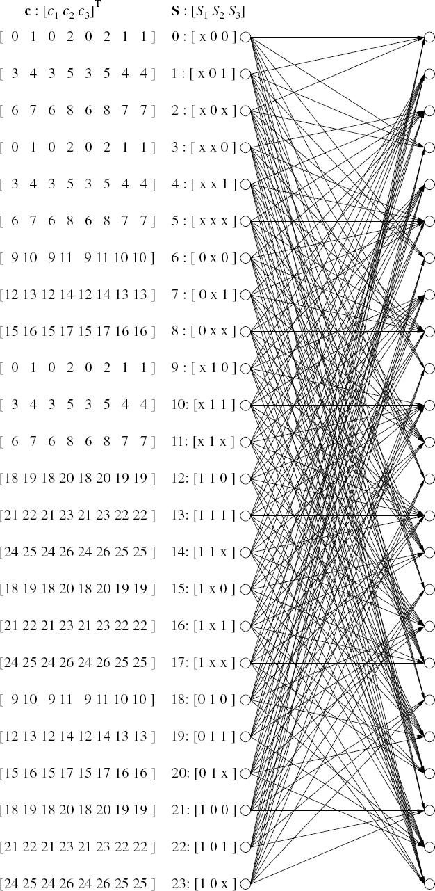
Figure 10.4: The VL-STCM-ID transmitter employing Nt = 3 transmit and Nr = 2 receive antennas, where πs denotes a symbol interleaver. © IEEE [271] Ng et al. 2007.
10.5 VL-STCM-ID Scheme
In order to invoke iterative detection and hence attain iteration gains as a benefit of the more meritoriously spread extrinsic information, we introduce a symbol-based random4 interleaver and a non-binary URC for each of the Nt = 3 transmit antennas. The Nt = 3 parallel symbol-based interleavers were generated independently. As we can see from Figure 10.4, each element in the space–time codeword cm[t] for m ∈ {1, 2, 3} is further interleaved and encoded by a non-binary URC, before being fed to the mapper. The convergence behavior of the iterative VL-STCM-ID decoder is analyzed in Section 10.6, where it is shown that the VL-STCM-ID scheme would be unable to converge at low SNRs, when the recursive feedback-assisted non-binary precoders or URCs are not used. In contrast, a simple single-cell non-binary URC invoked before the mapper of each transmit antenna would allow us to achieve a significant iteration gain. Hence, the VL-STC encoder was retained unaltered, but the original modulator was modified. The non-binary URC employs a modulo-![]() adder, where, again,
adder, where, again, ![]() = 3 is the number of different symbols in the VLC space–time codeword and we have cm[t] ∈ {0, 1, x}. Accordingly, this single-cell URC possesses
= 3 is the number of different symbols in the VLC space–time codeword and we have cm[t] ∈ {0, 1, x}. Accordingly, this single-cell URC possesses ![]() = 3 trellis states. Note that we represent the ‘x’ symbol using the number ‘2’ during the modulo-
= 3 trellis states. Note that we represent the ‘x’ symbol using the number ‘2’ during the modulo-![]() addition. Furthermore, the VL-STCM-ID scheme is very similar to the BICMID arrangement proposed in [329], where N parallel bit-based interleavers were used for interleaving the bits of the N-bit codeword before the modulator, in order to attain iteration gains. By contrast, the VL-STCM-ID scheme employs Nt parallel symbol-based interleavers for interleaving the symbols of the Nt-symbol space–time codeword before the modulator, in order to attain iteration gains with the aid of iterative decoding.
addition. Furthermore, the VL-STCM-ID scheme is very similar to the BICMID arrangement proposed in [329], where N parallel bit-based interleavers were used for interleaving the bits of the N-bit codeword before the modulator, in order to attain iteration gains. By contrast, the VL-STCM-ID scheme employs Nt parallel symbol-based interleavers for interleaving the symbols of the Nt-symbol space–time codeword before the modulator, in order to attain iteration gains with the aid of iterative decoding.
At the receiver, the symbol-based log-domain MAP algorithm [328] is used by both the VL-STC decoder and the URC decoder. The block diagram of the VL-STCM-ID receiver is depicted in Figure 10.5, where we denote the log-domain symbol probability of the VL-STC codeword cm and the URC codeword um for the mth transmitter as ![]() respectively. Furthermore, the subscripts a and e denote the a priori and extrinsic nature of the probabilities, while the superscript i.m suggests that the probabilities belong to the ith decoder stage of the mth transmitter. Note that i = 0 implies that the probabilities were calculated from the source symbol distribution.
respectively. Furthermore, the subscripts a and e denote the a priori and extrinsic nature of the probabilities, while the superscript i.m suggests that the probabilities belong to the ith decoder stage of the mth transmitter. Note that i = 0 implies that the probabilities were calculated from the source symbol distribution.
Figure 10.5: The VL-STCM-ID receiver for an Nr × Nt MIMO system. The notations ![]() and
and ![]() indicate the extrinsic and a priori probability and the hard decision estimate of (.), respectively. The notation
indicate the extrinsic and a priori probability and the hard decision estimate of (.), respectively. The notation ![]() denotes the log-domain symbol probability of the VL-STC codeword c or the URC codeword u for the mth transmitter. The subscripts a and e denote the a priori and extrinsic nature of the probabilities while the superscript i.m identifies that the probabilities belong to the ith stage decoder for the mth transmitter. Note that i = 0 means that the probabilities were calculated from the source symbol distribution. © IEEE [271] Ng et al. 2007.
denotes the log-domain symbol probability of the VL-STC codeword c or the URC codeword u for the mth transmitter. The subscripts a and e denote the a priori and extrinsic nature of the probabilities while the superscript i.m identifies that the probabilities belong to the ith stage decoder for the mth transmitter. Note that i = 0 means that the probabilities were calculated from the source symbol distribution. © IEEE [271] Ng et al. 2007.

The extrinsic probability of the URC codeword of transmit antenna m, namely Pe(um[t]), can be computed during each symbol period in the ‘Soft Demapper’ block of Figure 10.5. By dropping the time-related square bracket, we can compute Pe(um) as

where the subset χ(m, b) contains all the phasor combinations for the transmitted signal vector x = [x1 x2 · · · xNt]T where xm = f(um = b) holds, while P(y|x) is the Probability Density Function (PDF) of the MIMO Rayleigh fading channel given by
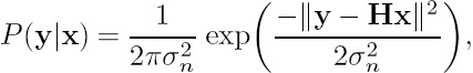
and σn2 = N0/2 is the noise variance and y is the Nr-element complex received signal vector, while H is an (Nr × Nt)-dimensional complex channel matrix during the time instant t. Furthermore, the a priori probability of um in Equation (10.10) is computed from the extrinsic log-domain probability of the mth URC MAP decoder as Pa(um) = exp(Le2.m(u)), while the log-domain a priori probability of um for the mth URC MAP decoder is given by L1.me(u) = ln(Pe(um)). Hence, the soft demapper benefits from the a priori information of its input symbols um after the first iteration. Note that we employ the Jacobian logarithm [330] to compute Equation (10.10) in the log domain; hence there is no need for log domain to normal domain conversion. As we can see from Figure 10.5, each of the Nt = 3URC MAP decoders seen inside the demodulator block benefits from the a priori information of its codeword um[t] as well as from that of its input symbol cm[t], m ∈ {1, 2,. .., Nt}.
It is possible to attain some a priori probability for the Nt-element VL-STC codewords, c, (which also constitute the URC’s input words), given the source symbol occurrence probability specified in Equation (10.4). Explicitly, the probability of the mth URC’s input word cm can be expressed as
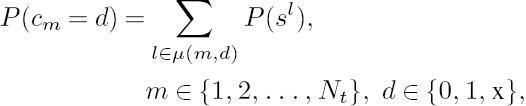
where the subset µ(m, d) contains the specific indices of those columns in the VLC matrix, where the mth row element in that column equals d. Hence, we have La0.m(c) = ln(P(cm)) as an additional a priori probability for symbol cm during each iteration between the URC MAP decoder and the VL-STC MAP decoder, as shown in Figure 10.5. Note that P(cm) is directly computed from the source symbol occurrence probability P(sl); hence we do not use P(sl) again as the a priori probability of the VL-STC input word in the VL-STC MAP decoder, in order to avoid reusing the same information. Therefore, both the VL-STC and the URC MAP decoders benefit from the a priori or extrinsic information of the space–time codeword c[t] = [c1[t]c2[t]c3[t]]T received from each other as well as from the additional a priori information provided by the potentially different probability source symbols s[t]. A full iteration consists of a soft demapper operation, Nt = 3URC MAP decoder operations and a VL-STC MAP decoder operation. For the non-iteratively decoded VL-STCM/FLSTCM, the soft demapper computes the a priori information of c[t] = [c1[t]c2[t]c3[t]]T and feeds it to the VL-STC/FL-STCM MAP decoder. Note that the VL-STC/FL-STC decoder of VL-STCM/FL-STCM also benefits from the a priori probability of its input word s[t], which is given by the source symbol occurrence probability in Equation (10.4). Hence, as the source becomes correlated, the VL-STCM-ID, VL-STCM and FL-STCM schemes will benefit from the a priori probability of the source symbols. However, FL-STCM attains no energy savings.
10.6 Convergence Analysis
EXtrinsic Information Transfer (EXIT) charts designed for binary receivers [331] have been widely used for analyzing the convergence behavior of iterative-decoding-aided concatenated coding schemes. The non-binary EXIT charts were introduced on the basis of the multidimensional histogram computation of [332, 333]. However, the convergence analysis of the proposed three-stage VL-STCM-ID scheme requires the employment of novel three-dimensional (3D) non-binary EXIT charts, which evolved from the binary 3D EXIT charts used in [334, 335] for analyzing multiple concatenated codes.
To elaborate a little further, EXIT charts visualize the input and output characteristics of the constituent MAP decoders in terms of the mutual information transfer between the input sequence and the a priori information at the input, as well as between the input sequence and the extrinsic information at the output of the constituent decoder. Hence, there are two steps in generating an EXIT chart. Firstly, we have to model the a priori probabilities of the input sequence and then feed it to the decoder. Secondly, we have to compute the mutual information of the extrinsic probabilities at the output of the decoder. Let us now model the a priori probabilities of the VL-STC codeword, c = [c1 c2 · · · cNt]T.
Let us assume that the input symbol of one of the URC encoders, denoted as c, is transmitted across an AWGN channel using the ![]() = 3-phasor mapper shown in Figure 10.2, and the received signal is given by y = x + n, where n is the AWGN noise having a zero mean and a variance of
= 3-phasor mapper shown in Figure 10.2, and the received signal is given by y = x + n, where n is the AWGN noise having a zero mean and a variance of ![]() . Furthermore, we have x = f(c), where f(.) is the mapper function portrayed in Figure 10.2. Since f(.) is a memoryless function, the probability of occurrence for x is the same as that of c. Hence, we have P(x) = P(c), which can be expressed from Equation (10.12). At a given probability of occurrence for x, the mutual information between x and y can be formulated as
. Furthermore, we have x = f(c), where f(.) is the mapper function portrayed in Figure 10.2. Since f(.) is a memoryless function, the probability of occurrence for x is the same as that of c. Hence, we have P(x) = P(c), which can be expressed from Equation (10.12). At a given probability of occurrence for x, the mutual information between x and y can be formulated as
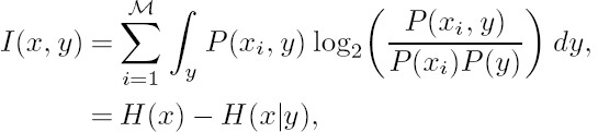
where H(x) is the entropy of x, given by
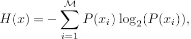
and H(x|y) is the conditional entropy of x given y, which can be expressed as
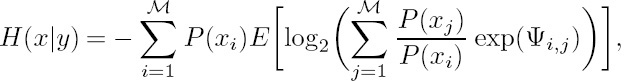
where exp(Ψi,j) = P(y|xi)/P (y|xj) and P(y|x) is the conditional Gaussian PDF, while the exponent Ψi,j is given by

The expectation term E [.] in Equation (10.15) is taken over different representations of the AWGN noise n.
Let us now denote the a priori information of c as IA(c) = I(x, y). Note that I(x, y) is monotonically decreasing with respect to ![]() and we can simplify Equation (10.13) to a form where I(x, y) is expressed as a function J(.) of
and we can simplify Equation (10.13) to a form where I(x, y) is expressed as a function J(.) of ![]() , i.e. as I(x, y) = J(
, i.e. as I(x, y) = J(![]() ). Hence, at a given IA value we can find the corresponding noise variance with the aid of the inverse function
). Hence, at a given IA value we can find the corresponding noise variance with the aid of the inverse function ![]() = J−1(IA(c)). Then we can generate a noise sample n′ having a variance of
= J−1(IA(c)). Then we can generate a noise sample n′ having a variance of ![]() . Consequently, we can produce y′ = x + n′, where again x = f(c) represents the mapper function portrayed in Figure 10.2 and c is the actual input symbol of the particular URC encoder. Finally, we can generate the a priori symbol probabilities for Pa(c) using the conditional Gaussian PDF:
. Consequently, we can produce y′ = x + n′, where again x = f(c) represents the mapper function portrayed in Figure 10.2 and c is the actual input symbol of the particular URC encoder. Finally, we can generate the a priori symbol probabilities for Pa(c) using the conditional Gaussian PDF:

for c ∈ {0, 1, x}. Then we feed these symbol probabilities to the corresponding MAP decoder. Note that the above method can be used for any symbol-interleaved serially concatenated coding schemes, where the symbol probabilities are directly created for a given IA value.
Next, we compute the mutual information of the extrinsic symbol probabilities IE(c) of the VL-STC or URC decoder output using the method proposed in [332] for the symbol c. Finally, the mutual information for the Nt-element VL-STC codeword c = [c1 c2 · · · cNt]T is expressed as the sum of mutual information valid for its symbol components cm, m ∈ {1, 2, ..., Nt}. Hence we have ![]() . We also compute the mutual information for the URC codeword u based on the same procedure. However, the experimentally evaluated histogram of u exhibited a near-uniform distribution (in other words, it was associated with equiprobable symbols) when the symbol interleaver length was sufficiently high. This is because the URC employed can be viewed as an accumulator.
. We also compute the mutual information for the URC codeword u based on the same procedure. However, the experimentally evaluated histogram of u exhibited a near-uniform distribution (in other words, it was associated with equiprobable symbols) when the symbol interleaver length was sufficiently high. This is because the URC employed can be viewed as an accumulator.
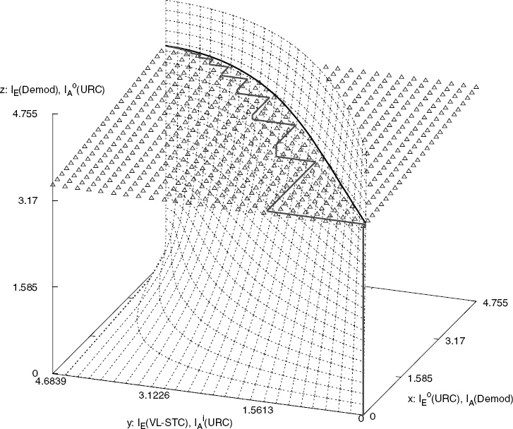
The 3D EXIT charts and the actual iterative decoding trajectories for the VL-STCMID scheme having Nt = 3 and Nr = 2 when using an uncorrelated source are shown in Figures 10.6 and 10.7 respectively. Let us denote the three axes of the 3D EXIT charts using the letters x, y and z, while IA(*) and IE(*) denote the a priori and extrinsic information for (*), respectively, where (*) is either the VL-STC MAP decoder (VL-STC) or the URC MAP decoder (URC) or, alternatively, the soft demapper (Demod). As we can see from Figure 10.5, each of the URC MAP decoders takes (provides) the a priori (extrinsic) probabilities of its input word c and output word (or codeword) u as the input (output). Hence, the mutual information of the input word and output word of the URC decoder will be represented by Ii(A, E) (URC) and Io(A, E) (URC), respectively. Each of the Nt symbol interleavers shown in Figure 10.4 has a length of 10 000 symbols.
The EXIT plane marked with triangles in Figure 10.6 was computed based on the extrinsic probabilities of the soft demapper L1e.m(u), for m ∈ {1, 2, 3}, at the given values in the x and y axes at Eb/N0 = 4 dB. The other EXIT plane marked with dashed lines in Figure 10.6 is SNR-independent and was plotted based on the URC decoders’ output word extrinsic probabilities L2.me(u), for m ∈ {1, 2, 3}, at the given values in the y and z axes. The decoding trajectory, which was determined based on the extrinsic probabilities Le1.m(u), L2e.m(u) and L3.me(c) for m ∈ {1, 2, 3} as in Figure 10.5, is under the EXIT plane marked with triangles and on the left of the EXIT plane marked with dashed lines in Figure 10.6.
Figure 10.7 depicts the 3D EXIT charts, when the x axis of Figure 10.6 is changed from IoE(URC) to IiE(URC). More explicitly, the vertical EXIT plane seen in Figure 10.7, which
Figure 10.6: The 3D EXIT charts for the VL-STCM-ID scheme having Nt = 3 and Nr = 2, when using an uncorrelated source. The iterative trajectory is computed at Eb/N0 = 4 dB. © IEEE [271] Ng et al. 2007.
is independent of the z axis and the SNR, was computed based on the VL-STC decoder’s extrinsic probabilities L3.me(c), for m ∈ {1, 2, 3}, at the given values in the x and z axes. The slanted EXIT plane shown in Figure 10.7 is also SNR independent and was computed based on the URC decoders’ input word extrinsic probabilities L2.me(c), for m ∈ {1, 2, 3}, at the given values in the y and z axes. The stepwise-linear iterative decoding trajectory displayed in Figure 10.7 was plotted based on the extrinsic probabilities Le1.m(u), L2e.m(c) and Le3.m(c) for m ∈ {1, 2, 3}.
According to [335], the intersection of the planes in Figure 10.6 represents the points of convergence between the soft demapper and the URC decoder. The intersection points, where we have IA(Demod) = IoE(URC) at the corresponding IiA(URC) and IoA(URC) values, are shown in Figure 10.6 as a solid line. The corresponding values of IiE(URC) are shown in Figure 10.7 as a solid line on the slanted EXIT plane. Similarly, the intersection of the EXIT planes seen in Figure 10.7 represents the points of convergence between the URC decoder and the VL-STC decoder. Hence, projecting these two intersection curves onto z = 0 in Figure 10.7 gives us the equivalent 2D EXIT chart seen in Figure 10.8. Therefore, the 3D EXIT charts generated for multiple concatenated codes can be projected onto an equivalent 2D EXIT chart [335].
More specifically, we can observe an open tunnel between the EXIT curves of the VLSTC and URC schemes in the 2D EXIT charts of Figure 10.8 at Eb/N0 = 4 dB, which indicates that decoding convergence can be achieved. However, the URC EXIT curve is
Figure 10.7: The 3D EXIT charts for the VL-STCM-ID scheme having Nt = 3 and Nr = 2, when using an uncorrelated source. The iterative trajectory is computed at Eb/N0 = 4dB. © IEEE [271] Ng et al. 2007.
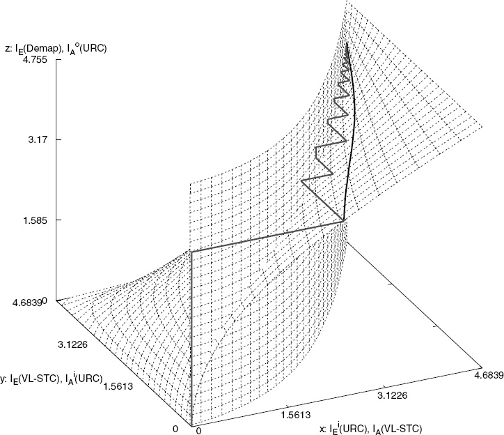
Figure 10.8: The 2D EXIT charts projection for the VL-STCM-ID scheme having Nt = 3 and Nr = 2, when using an uncorrelated source. The iterative trajectory is computed at Eb/N0 = 4dB. © IEEE [271] Ng et al. 2007.
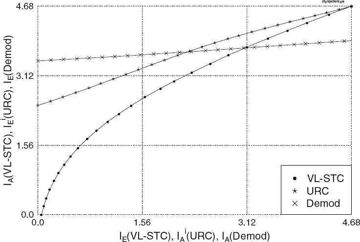
SNR dependent, and by reducing the Eb/N0 values the angle between the two curves at the top right-hand corner would be further reduced, and hence the open tunnel would become closed, preventing decoding convergence. Therefore, a better URC code may be designed by ensuring that the EXIT curve exhibits a wider angle with respect to the VL-STC EXIT curve. Note, furthermore, that the EXIT curve generated for the soft demapper is also depicted in Figure 10.8 at Eb/N0 = 4dB, where it is flat and it intersects with the VL-STC EXIT curve, before the maximum value of 4.68 bits is reached. Hence, decoding convergence cannot be achieved at Eb/N0 = 4dB, when the URC was not invoked between the soft demapper and the VL-STC. Furthermore, at IE (VL-STC) = 0 we have IiE(URC) < IE (Demod). Therefore, before any iteration feedback is exploited, the VL-STCM-ID scheme would not outperform its VL-STCM counterpart. It was also concluded in [334] that for a three-stage serially concatenated system a unity-rate recursive encoder, such as the URC used, should be employed at the intermediate stage in order to achieve optimal decoding convergence.
Figure 10.9 shows the 3D EXIT charts and the corresponding convergence curve of the soft demapper and the URC decoder as well as the actual iterative decoding trajectory for the VL-STCM-ID scheme having Nt = 3 and Nr = 2when using the correlated source defined in Equation (10.4). As the source becomes correlated, the entropy of the codeword cm for m ∈ {1, 2, 3} reduces. Hence, the maximum values for the x and y axes in Figure 10.9 are smaller than those in Figure 10.7. However, the open spatial segment of the 3D space between the two EXIT planes becomes wider when the source is correlated, since the decoders exploit the additional a priori probabilities given by Equation (10.12).
The convergence curve of the soft demapper and the URC decoder is projected as a dashed line onto IE (Demod) = 0in Figure 10.9. Similarly, the projection of the intersection line between the VL-STC and URC EXIT planes is represented by the curve lying on the vertical EXIT plane at IE (Demod) = 0. As can be seen from Figure 10.9 at IE (Demod) = 0, an open tunnel exists between the two projection curves at Eb/N0 = 3 dB. Hence, the iterative decoder converged at Eb/N0 = 3dB, i.e. at a 1 dB lower value, when employing the correlated source instead of the uncorrelated source. Again, the decoding convergence of VLSTCM-ID is limited by the angle between the two projection curves at the convergence point when using the correlated source. A better URC may be designed for an earlier convergence with the aid of the 3D and 2D EXIT charts, but we leave this issue for future research.
According to the MIMO channel capacity formula derived for the Discrete-input Continuous-output Memoryless Channel (DCMC) in [336], the DCMC capacity for the Nr = 2 and Nt = 3 MIMO scheme employing the signal mapper seen in Figure 10.2 is Eb/N0 = 1.25 dB at a bandwidth efficiency of 3 bit/s/Hz. Hence, the performance of the VL-STCM-ID scheme is about 2.75 dB and 1.75 dB away from the MIMO channel capacity.
10.7 Simulation Results
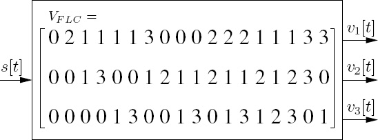
Let us introduce a Fixed Length (FL) STCM (FL-STCM) scheme as our benchmark, where the FL codeword matrix is given by
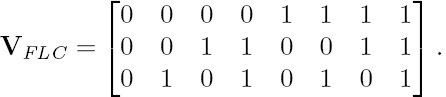
Figure 10.9: The 3D EXIT charts for the VL-STCM-ID scheme having Nt = 3 and Nr = 2, when using the correlated source defined in Equation (10.4). The iterative trajectory is computed at Eb/N0 = 3 dB. © IEEE [271] Ng et al. 2007.

The FL-STCM transmitter obeys the schematic of Figure 10.1, except that it employs the VFLC of Equation (10.18). For the FL-STCM, the minimum Hamming distance and product distance are 1 and 4, respectively. It attains the same multiplexing gain as that of the VL-STCM or VL-STCM-ID arrangements. Note that it is possible to create an iterative FL-STCM-ID scheme by replacing the VL-STC encoder in Figure 10.4 with the FL-STC encoder. However, the EXIT curve of the FL-STC scheme of Equation (10.18) was found to be too flat for attaining any iteration gain due to its unity minimum Hamming distance. Let us now evaluate the performance of the VL-STCM, VL-STCM-ID and FL-STCM schemes in terms of their source Symbol-Error Ratio (SER) versus the Eb/N0 ratio. Again we have Eb/N0 = γ/η, where γ is the SNR per receive antenna and η =log2(Ns) = 3bit/s/Hz is the effective information throughput.
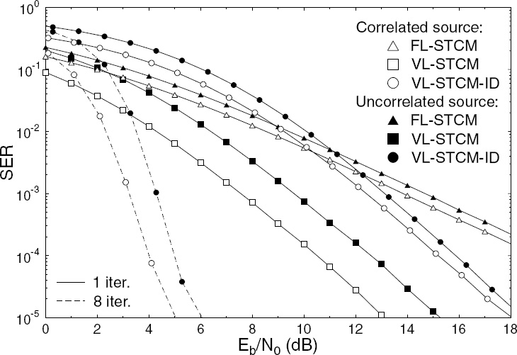
Figure 10.10 depicts the SER versus Eb/N0 performance of the VL-STCM, VLSTCM-ID and FL-STCM schemes, when communicating over uncorrelated Rayleigh fading channels using BPSK, three transmitters, two receivers and a block/interleaver length of 10 000 symbols. As expected, the VL-STCM arrangement attains a higher gain when the source is correlated compared with FL-STCM. However, the FL-STCM benchmark also benefits from the probability-related a priori information of the source symbols as the source becomes correlated. Both the FL-STCM and VL-STCM-ID schemes also manage to achieve some coding gain, since their decoder benefits from the probability-related a priori information of the source symbols. By contrast, the coding gain attained as a benefit of transmitting correlated source symbols increases as the number of iterations invoked by the VL-STCM-ID scheme increases. Although the VL-STCM-ID arrangement performs worse than VL-STCM during the first iteration, the performance of VL-STCM-ID at SER = 10−4 after the eighth iteration is approximately 6.5 (15) dB and 7.5 (14.6) dB better than that of the VL-STCM (FL-STCM) scheme, when employing correlated and uncorrelated sources respectively. The price of using the VL-STCM-ID scheme for attaining a near-channel-capacity performance is the associated higher decoding and interleaver delay as well as the increased decoding complexity. Hence, for a delay-sensitive and complexity-constrained system, using VL-STCM is a better choice. By contrast, for a system that requires a higher performance and can afford a higher delay and complexity, VL-STCM-ID should be employed.
Figure 10.10: SER versus Eb/N0 performance of the VL-STCM, VL-STCM-ID and FLSTCM schemes, when communicating over uncorrelated Rayleigh fading channels using BPSK, Nt = 3 and Nr = 2. © IEEE [271] Ng et al. 2007.
10.8 Non-Binary VL-STCM
In this section, we will show that our VLC-STCM design can be extended to higher-order modulation schemes for attaining a higher throughput. More specifically, we will design a non-binary VL-STCM scheme using 2D non-binary VLCs. Similar to the binary VL-STCM scheme, the number of activated transmit antennas in the non-binary VL-STCM encoder equals the number of non-binary symbols of the corresponding VLC codeword in the spatial domain, where each VLC codeword is transmitted during a single symbol period. Hence, the transmission frame length is determined by the fixed number of source symbols and therefore this non-binary VL-STCM scheme does not exhibit synchronisation problems and does not require the transmission of side information.
10.8.1 Code Design
Figure 10.11: The Ns = 18 possible VLC codewords v[t] of the codeword matrix in the 2D non-binary VLC VVLC employing 4PSK modulation, which signals the Ns = 18 possible source symbols with the aid of using Nt = 3 transmit antennas.
The block diagram of the non-binary VL-STCM transmitter is similar to Figure 10.1 except that a 2D non-binary VLC encoder is used. An example of the 2D non-binary VLC codeword matrix, VVLC, is depicted in Figure 10.11 when there are Ns = 18 possible source symbols and Nt = 3 transmit antennas. More explicitly, each column of the (3 × 18) dimensional matrix VVLC corresponds to one codeword and the elements in the matrix represent the 4PSK symbols to be transmitted by the different antennas, while ‘x’ represents ‘no transmission’. ‘No transmission’ implies that the corresponding transmitter antenna sends no signal. The VLC codeword v[t] corresponding to source symbol s[t] = j, j = 1, 2,. .. ,18, at time instant t is given by the jth column of the matrix VVLC. Hence, each of the Nt = 3 components of v[t] may assume one of the following values vi[t] ∈ {x, 0, 1, 2, 3}, where i ∈ {1, 2, ..., Nt} when 4PSK modulation is employed5. Note that more transmission energy is saved, which may be reallocated to ‘active’ symbols, when there are more ‘no transmission’ symbols in a VLC codeword v[t]. Therefore, the columns of the matrix VVLC, which are the VLC codewords, and the source symbols are specifically arranged, so that the more frequently occurring source symbols are assigned to VLC codewords having more ‘no transmission’ components, in order to save transmit energy.
The signal mapper blocks of the non-binary VL-STCM scheme are characterized in Figure 10.12. Again, the ‘no transmission’ symbol is represented by the origin of the Euclidean space. Furthermore, the amount of energy saving can be computed from Eq. (10.7) as before. where Lave is the average codeword length of the VLC codeword matrix VVLC. As an example, we use the Ns = 18 source symbol probabilities of P(s) = {0.1776, 0.158, 0.1548, 0.1188, 0.1162, 0.077, 0.0682, 0.0388, 0.0374, 0.0182, 0.017, 0.0068, 0.0066, 0.002, 0.0016, 0.0007, 0.0002, 0.0001}. Hence, the average codeword length is given by Lave = ![]() = 1.5208 for the VVLC matrix of Figure 10.11, where L(s) is the number of ‘active’ transmitted symbols in the VLC codeword assigned to source symbol s according to Figure 10.11. Hence, in this specific example a power saving of
= 1.5208 for the VVLC matrix of Figure 10.11, where L(s) is the number of ‘active’ transmitted symbols in the VLC codeword assigned to source symbol s according to Figure 10.11. Hence, in this specific example a power saving of ![]() dB can be obtained. Note however that the more correlated the source, the lower the average codeword length, and hence the higher the power saving. In order to normalize the average energy of the multiple transmitter-based modulation constellations to unity, we have to scale the 4PSK constellation of each transmitters such that the radius of the 4PSK constellation becomes
dB can be obtained. Note however that the more correlated the source, the lower the average codeword length, and hence the higher the power saving. In order to normalize the average energy of the multiple transmitter-based modulation constellations to unity, we have to scale the 4PSK constellation of each transmitters such that the radius of the 4PSK constellation becomes ![]() .
.
Figure 10.12: The signal mapper of the non-binary VL-STCM.
As we can see from Figures. 10.1 and 10.11, each of the 18 non-binary VLC codewords v[t] = [v1[t] v2[t] v3[t]]T is transmitted using Nt = 3 transmitters, where the mth element of each VLC codeword, for 1 ≤ m ≤ Nt, is delayed by (m − 1) shift register cells, before it is transmitted through the mth transmit antenna. Hence, the Nt number of components of each VLC codeword are transmitted on a diagonal of the spacetime codeword matrix of Equation (10.2). Since the VLC codewords are transmitted diagonally, the transmitted signal at the mth antenna, for 1 ≤ m ≤ Nt, at a particular time-instant t is given by xm[t] = f(vm [t − m + 1]). Hence, for the spacetime codeword matrix of Equation (10.2) can be written as:

It can be shown based on [325] that the minimum Hamming distance EH of the VL-STCM scheme is given by:
where dHVLC is the symbol-based minimum Hamming distance of the 2D VLC employed. The symbol-based Hamming distance between any two VLC codewords, which are selected from the columns of the codeword matrix VVLC of Figure 10.11, is given by the number of different symbols -rather than bits -between the two VLC codewords. For example, the symbol-based Hamming distance between the first and the last columns of VVLC shown in Figure 10.11 is three, where the ‘no transmission’ symbol ‘x’ is included as the fifth symbol. The minimum product distance EP min is given by Equation (10.8).
In the example of Figure 10.11 we have EH min = dHVLC = 2 and EP min = 3.89, which were found to be the maximum achievable values at Ns = 18 and Nt = 3 by our exhaustive computer search for the best solution. Furthermore, the effective throughput of the VL-STCM scheme is given by log2(Ns) = 4.17 bits per symbol (bps), which is significantly higher than log2(4) = 2 bps in the case of classic 4PSK modulation. Therefore, firstly a transmit diversity order of EH min = 2 was attained. Secondly, a coding advantage directly related to the value of EP min = 3.89 was achieved. Thirdly, a multiplexing gain can also be attained for Ns > M, where M is the number of modulation levels in the original modulation scheme. Additionally, the correlation of the source only affects the specific mapping of the different-probability source symbols to the 2D VLC codewords of Figure 10.11, but not the design of the 2D VLC itself. Therefore, the higher the source correlation, the lower the average codeword length Lave. Hence, a higher power saving can be obtained, when the source is more correlated, since the amount of energy saving is given by Equation (10.7), where Nt is fixed.
10.8.2 Benchmarker
Figure 10.13: The codeword matrix of the 2D non-binary FLC CFLC employing 4PSK modulation, having Ns = 18 number of possible source symbols and using Nt = 3 transmit antennas.
In order to benchmark the proposed VL-STCM scheme of Figure 10.11, a Fixed-Length STCM (FL-STCM) benchmarker was created. The codeword matrix of the Fixed Length Code (FLC) is shown in Figure 10.13, where again, 4PSK modulation was employed in conjunction with Ns = 18 and Nt = 3. In the FLC all Nt transmit antennas are active at all time instants, hence there are only M = 4 phasors in the modulation constellation and no power saving is achieved due to the absence of ‘no transmission’ symbols. Similar to the VLC scheme of Figure 10.11, this was designed by exhaustive computer search, evaluating Equations. 10.19 and 10.8 for all possible combinations of the 4PSK symbols.
At Ns = 18, we have EH min = 1 and EP min = 2, which are the maximum achievable values for the FLC at a given combination of Ns = 18 and Nt = 3. However, these values are significantly smaller than the EH min and EP min of the 2D VLC. Nonetheless, both FL-STCM and VL-STCM achieve the same multiplexing gain of log2(Ns/M) = 2.17 due to having the same average throughput of log2(Ns) = 4.17 bps when compared to the 4PSK (M = 4) modulation.
10.8.3 Decoding
At the receiver, both the Viterbi and the MAP algorithms may be used by the trellis-based decoder. The trellis states are defined by the contents of the shift register cells D shown in Figure 10.1. Note that each shift register cell may hold five possible values, namely { x, 0, 1, 2, 3} for the non-binary VL-STCM and four 4PSK values for the non-binary FLSTCM scheme. However, not all consecutive state sequences are possible due to the constraint imposed by the 2D VLC of Figure 10.11 or by the FLC code of Figure 10.13. More specifically, there are 90 and 44 possible trellis states in the trellis of the VL-STCM and FL-STCM schemes, respectively. Hence, the decoding complexity of the VL-STCM based on the VVLC matrix of Figure 10.11 is about twice that of the FL-STCM based on the CFLC matrix of Figure 10.13. The log-domain symbol metrics can be computed based on the PDF of the channel as:
where y[t] = [y1[t] ... yNr[t]] is the received signal vector at time-instant t, x[t] = [x1[t] ... xNt[t]] is the Nt-element space-time coded symbol and xm[t] = f(vm[t − m + 1]). When the different source symbols’ probability of occurrence P(d) is different, it can be used as the a priori probability for assisting the trellis decoder. Hence, the log-domain trellis branch transition metrics of the transition from the previous state S−1 to the current state S may be computed as:
where x[t] and s are the associated codeword and source symbol for that trellis branch, while Pr (y[t]|x[t]) is given by Equation (10.20) and Pr(s) = ln P(s) is the log-domain a priori probability of the source symbol s.
It is worth mentioning that it is possible to design a VL-STCM scheme, which has a higher minimum product distance, EP min, at the cost of a higher decoding complexity. More explicitly, the design of the proposed VL-STCM is based on the search for an optimum nonbinary 2D VLC matrix VVLC, as shown in Figure 10.11, and its trellis is based on the shift-registers shown in Figure 10.1. By contrast, a VL-STCM scheme having a higher EP min can be designed based on the search of an optimum space-time codeword matrix X, given by Equation (10.2), using a trellis that has a higher number of trellis states.
10.8.4 Simulation results
Let us now evaluate the performance of both the VL-STCM and FL-STCM schemes in terms of their source SER versus the SNR per bit, which is given by Eb/N0 = γ/η, where γ is the SNR per receive antenna and η = log2(18) = 4.17 bps is the effective information throughput.
Figure 10.14 depicts the SER versus Eb/N0 performance of the VL-STCM and FL-STCM schemes, when communicating over uncorrelated Rayleigh fading channels using 4PSK, three transmitters and two receivers. Note that when the source is uncorrelated, we have Lave = 2.1667 and ![]() for the VL-STCM scheme, hence the power saving of VL-STCM is given by 20 log10(A0) = 1.4133 dB and the effective product distance is given by EP min = 1.92. By contrast, the results for the correlated source investigated are based on the source symbol probabilities P(s) defined in Section 10.8.1. The upper bounds of the PWEP defined in Equation (10.3) are also shown in Figure 10.14 for comparison with the simulation results. As we can see from Figure 10.14, the performance of VL-STCM is about 1.7 dB better, when the source is correlated as compared to when the source is uncorrelated. This is due to the higher achievable EP min value, when the source is correlated. Observe in Figure 10.14 that the PWEP upper bounds of the VL-STCM are close to the simulation results. By contrast, the performance of the FL-STCM is about 1.1 dB better, when the source is correlated compared to the uncorrelated source. This is because the branch transition metrics in Equation (10.21) benefit from the different source symbol probabilities, when the source is correlated.
for the VL-STCM scheme, hence the power saving of VL-STCM is given by 20 log10(A0) = 1.4133 dB and the effective product distance is given by EP min = 1.92. By contrast, the results for the correlated source investigated are based on the source symbol probabilities P(s) defined in Section 10.8.1. The upper bounds of the PWEP defined in Equation (10.3) are also shown in Figure 10.14 for comparison with the simulation results. As we can see from Figure 10.14, the performance of VL-STCM is about 1.7 dB better, when the source is correlated as compared to when the source is uncorrelated. This is due to the higher achievable EP min value, when the source is correlated. Observe in Figure 10.14 that the PWEP upper bounds of the VL-STCM are close to the simulation results. By contrast, the performance of the FL-STCM is about 1.1 dB better, when the source is correlated compared to the uncorrelated source. This is because the branch transition metrics in Equation (10.21) benefit from the different source symbol probabilities, when the source is correlated.
Figure 10.14: SER versus Eb/N0 performance of the VL-STCM and FL-STCM schemes, when communicating over uncorrelated Rayleigh fading channels using 4PSK, Nt = 3 and Nr = 2.
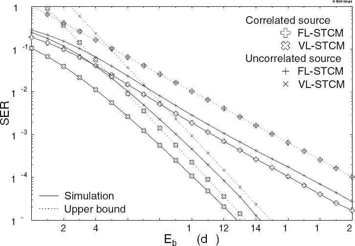
By comparing the simulation performance of VL-STCM and FL-STCM at SER = 10−4, the performance of VL-STCM is approximately 6 dB and 5.4 dB better than that of FLSTCM, when employing correlated and uncorrelated sources, respectively. Again, this coding gain is achieved at the cost of approximately doubling the decoding complexity from 44 to 90 trellis states.
10.9 Conclusions
An iteratively decoded variable-length space–time coded modulation design was proposed. The joint design of source-coding, space–time coded modulation and iterative decoding was shown to achieve both spatial diversity and multiplexing gain, as well as coding and iteration gains at the same time. The variable-length structure of the individual codewords mapped to the maximum of Nt transmit antennas imposes no synchronization and error propagation problems. The convergence properties of the proposed VL-STCM-ID were analyzed using 3D symbol-based EXIT charts as well as 2D EXIT chart projections. A significant iteration gain was achieved by the VL-STCM-ID scheme, which hence outperformed both the non-iterative VL-STCM scheme and the FL-STCM benchmark with the aid of Nt unity-rate recursive feedback precoders. The VL-STCM-ID scheme attains a near-MIMO channel capacity performance.
The proposed VL-STCM design may also be employed in the context of higher-order modulation schemes by first designing a two-dimensional VLC mapping high-order modulation constellations to the Nt transmit antennas. A non-binary VLC-STCM was designed and analyzed in Section 10.8, where an overall performance gain of 6 dB was attained by the non-binary VL-STCM scheme over the non-binary FL-STCM benchmarker scheme at SER = 10−4 when aiming for a throughput of 4.17 bps. The non-binary VL-STCM may also be extended to a non-binary VL-STCM-ID scheme for the sake of attaining further iteration gains. Our future research will incorporate both explicit channel coding and real-time multimedia source codecs.
1Part of this chapter is based on [271] © IEEE (2007).
2The spatial-diversity order is the product of the transmitter-diversity order and the receiver-diversity order.
3A space–time codeword is defined as the Nt-element output word of the VL-STC encoder of Figure 10.1.
4The optimization of the interleaver is not considered in this chapter.
5At this early phase of the research we set aside the related crest-factor problems for future work.