Chapter 2

Information Theory Basics

2.1 Issues in Information Theory

The ultimate aim of telecommunications is to communicate information between two geographically separated locations via a communications channel, with adequate quality. The theoretical foundations of information theory accrue from Shannon’s pioneering work [133, 215–217], and hence most tutorial interpretations of his work over the past fifty years rely fundamentally on [133, 215–217]. This chapter is no exception in this respect. Throughout the chapter we make frequent references to Shannon’s seminal papers and to the work of various authors offering further insights into Shannonian information theory. Since this monograph aims to provide an all-encompassing coverage of video compression and communications, we begin by addressing the underlying theoretical principles using a light-hearted approach, often relying on worked examples.

Early forms of human telecommunications were based on smoke, drum or light signals, bonfires, semaphores and the like. Practical information sources can be classified as analog and digital. The output of an analog source is a continuous function of time, such as, for example, the air pressure variation at the membrane of a microphone due to someone talking. The roots of Nyquist’s sampling theorem are based on his observation of the maximum achievable telegraph transmission rate over bandlimited channels [218]. In order to be able to satisfy Nyquist’s sampling theorem the analog source signal has to be bandlimited before sampling. The analog source signal has to be transformed into a digital representation with the aid of time-and amplitude-discretization using sampling and quantization.

The output of a digital source is one of a finite set of ordered, discrete symbols often referred to as an alphabet. Digital sources are usually described by a range of characteristics, such as the source alphabet, the symbol rate, the symbol probabilities, and the probabilistic interdependence of symbols. For example, the probability of ‘u’ following ‘q’ in the English language is p = 1, as in the word ‘equation.’ Similarly, the joint probability of all pairs of consecutive symbols can be evaluated.

In recent years, electronic telecommunications have become prevalent, although most information sources provide information in other forms. For electronic telecommunications, the source information must be converted to electronic signals by a transducer. For example, a microphone converts the air pressure waveform p(t) into voltage variation v(t), where

(2.1)

and the constant c represents a scaling factor, while τ is a delay parameter. Similarly, a video camera scans the natural three-dimensional scene using optics, and converts it into electronic waveforms for transmission.

The electronic signal is then transmitted over the communications channel and converted back to the required form; this may be carried out, for example, by a loudspeaker. It is important to ensure that the channel conveys the transmitted signal with adequate quality to the receiver in order to enable information recovery. Communications channels can be classified according to their ability to support analog or digital transmission of the source signals in a simplex, duplex or half-duplex fashion over fixed or mobile physical channels constituted by pairs of wires, Time Division Multiple Access (TDMA) time-slots, or a Frequency Division Multiple Access (FDMA) frequency slot.

The channel impairments may include superimposed, unwanted random signals, such as thermal noise, crosstalk via multiplex systems from other users, and interference produced by human activities (for example, car ignition or fluorescent lighting) and natural sources such as lightning. Just as the natural sound pressure wave between two conversing persons will be impaired by the acoustic background noise at a busy railway station, the reception quality of electronic signals will be affected by the unwanted electronic signals mentioned above. In contrast, distortion manifests itself differently from additive noise sources, since no impairment is explicitly added. Distortion is more akin to the phenomenon of reverberating loudspeaker announcements in a large, vacant hall, where no noise sources are present.

Some of the channel impairments can be mitigated or counteracted; others cannot. For example, the effects of unpredictable additive random noise cannot be removed or ‘subtracted’ at the receiver. They can be mitigated by increasing the transmitted signal’s power, but the transmitted power cannot be increased without penalties, since the system’s nonlinear distortion rapidly becomes dominant at higher signal levels. This process is similar to the phenomenon of increasing the music volume in a car parked near a busy road to a level where the amplifier’s distortion becomes annoyingly dominant.

In practical systems, the Signal-to-Noise Ratio (SNR), quantifying the wanted and unwanted signal powers at the channel’s output, is a prime channel parameter. Other important channel parameters are its amplitude and phase response, determining its usable bandwidth (B), over which the signal can be transmitted without excessive distortion. Among the most frequently used statistical noise properties are the Probability Density Function (PDF), the Cumulative Density Function (CDF), and the Power Spectral Density (PSD).

The fundamental communications system design considerations are whether a high-fidelity (hi-fi) or just acceptable video or speech quality is required from a system (this predetermines, among other factors, its cost, bandwidth requirements and the number of channels available, and has implementational complexity ramifications), and, equally important, the issues of robustness against channel impairments, system delay and so on. The required transmission range and worldwide roaming capabilities, the maximum available transmission speed in terms of symbols per second, information confidentiality, reception reliability, and the requirement for a convenient lightweight, solar-charged design, are similarly salient characteristics of a communications system.

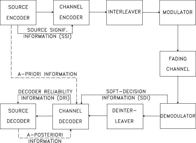
Information theory deals with a variety of problems associated with the performance limits of an information transmission system, such as the one depicted in Figure 2.1. The components of this system constitute the subject of this monograph; hence they will be treated in greater depth later in this volume. Suffice it to say at this stage that the transmitter seen in Figure 2.1 incorporates a source encoder, a channel encoder, an interleaver and a modulator, and their inverse functions at the receiver. The ideal source encoder endeavors to remove as much redundancy as possible from the information source signal without affecting its source representation fidelity (i.e., distortionlessly), and it remains oblivious of such practical constraints as a finite delay and limited signal processing complexity. In contrast, a practical source encoder will have to retain a limited signal processing complexity and delay while attempting to reduce the source representation bit rate to as low a value as possible. This operation seeks to achieve better transmission efficiency, which can be expressed in terms of bit-rate economy or bandwidth conservation.

The channel encoder re-inserts redundancy or parity information but in a controlled manner, in order to allow error correction at the receiver. Since this component is designed to ensure the best exploitation of the re-inserted redundancy, it is expected to minimize the error probability over the most common channel, namely the so-called Additive White Gaussian Noise (AWGN) channel, which is characterized by a memoryless, random distribution of channel errors. However, over wireless channels, which have recently become prevalent, the errors tend to occur in bursts due to the presence of deep received signal fades induced by the destructively superimposed multipath phenomena. This is why our schematic of Figure 2.1 contains an interleaver block, which is included in order to randomize the bursty channel errors. Finally, the modulator is designed to ensure the most bandwidth-efficient transmission of the source-and channel-encoded interleaved information stream, while maintaining the lowest possible bit error probability.

The receiver simply carries out the corresponding inverse functions of the transmitter.

Observe in the figure that, besides the direct interconnection of the adjacent system components, there are a number of additional links in the schematic. These will require further study before their role can be highlighted. At the end of this chapter we will return to this figure and guide the reader through its further intricate details.

Some fundamental problems transpiring from the schematic of Figure 2.1, which have been addressed in depth in a range of studies by Shannon [133, 215–217], Nyquist [218], Hartley [219], Abramson [220], Carlson [221], Raemer [222], Ferenczy [223] and others, are as follows.

• What is the true information generation rate of our information sources? If we know the answer, the efficiency of coding and transmission schemes can be evaluated by comparing the actual transmission rate used with the source’s information emission rate. The actual transmission rate used in practice is typically much higher than the average information delivered by the source, and the closer these rates are, the better is the coding efficiency.
• Given a noisy communications channel, what is the maximum reliable information transmission rate? The thermal noise induced by the random motion of electrons is present in all electronic devices, and if its power is high it can seriously affect the quality of signal transmission, allowing information transmission only at low rates.
• Is the information emission rate the only important characteristic of a source, or are other message features, such as the probability of occurrence of a message and the joint probability of occurrence for various messages, also important?

In a wider context, the topic of this whole monograph is related to the blocks of Figure 2.1 and to their interactions, but in this chapter we lay the theoretical foundations of source and channel coding as well as transmission issues, and define the characteristics of an ideal Shannonian communications scheme.

Although there are numerous excellent treatises on these topics that treat the same subjects with a different flavor [221, 223, 224], our approach is similar to that of the above-mentioned classic sources; since the roots are in Shannon’s work, references [133, 215–217, 225, 226] are the most pertinent and authoritative sources.

In this chapter we consider mainly discrete sources, in which each source message is associated with a certain probability of occurrence, which might or might not be dependent on previous source messages. Let us now give a rudimentary introduction to the characteristics of the AWGN channel, which is the predominant channel model in information theory due to its simplicity. The analytically less tractable wireless channels will be modeled mainly by simulations in this monograph.

2.2 Additive White Gaussian Noise Channel

2.2.1 Background

In this section we consider the communications channel, which exists between the transmitter and the receiver, as shown in Figure 2.1. Accurate characterization of this channel is essential if we are to remove the impairments imposed by the channel using signal processing at the receiver. Here we initially consider only fixed communications links, where both terminals are stationary, although mobile radio communications channels, which change significantly with time, are becoming more prevalent.

We define fixed communications channels to be those between a fixed transmitter and a fixed receiver. These channels are exemplified by twisted pairs, cables, wave guides, optical fiber and point-to-point microwave radio channels. Whatever the nature of the channel, its output signal differs from the input signal. The difference might be deterministic or random, but it is typically unknown to the receiver. Examples of channel impairments are dispersion, nonlinear distortions, delay and random noise.

Fixed communications channels can often be modeled by a linear transfer function, which describes the channel dispersion. The ubiquitous additive white Gaussian noise is a fundamental limiting factor in communications via Linear Time-Invariant (LTI) channels. Although the channel characteristics might change due to factors such as aging, temperature changes and channel switching, these variations will not be apparent over the course of a typical communication session. It is this inherent time invariance that characterizes fixed channels.

An ideal, distortion-free communications channel would have a flat frequency response and linear phase response over the frequency range of −∞ · · · + ∞, although in practice it is sufficient to satisfy this condition over the bandwidth (B) of the signals to be transmitted, as seen in Figure 2.2. In this figure, A(ω)represents the magnitude of the channel response at frequency ω, and ϕ (ω) = wT represents the phase shift at frequency ω due to the circuit delay T.

Practical channels always have some linear distortions due to their bandlimited, nonflat frequency response and nonlinear phase response. In addition, the group-delay response of the channel, which is the derivative of the phase response, is often given.

2.2.2 Practical Gaussian Channels

Conventional telephony uses twisted copper wire pairs to connect subscribers to the local exchange. The bandwidth is approximately 3.4 kHz, and the waveform distortions are relatively benign.

For applications requiring a higher bandwidth, coaxial cables can be used. Their attenuation increases approximately with the square root of the frequency. Hence, for wideband, long-distance operation, they require channel equalization. Typically, coaxial cables can provide a bandwidth of about 50 MHz, and the transmission rate they can support is limited by the so-called skin effect.

Point-to-point microwave radio channels typically utilize high-gain directional transmit and receive antennas in a line-of-sight scenario, where free-space propagation conditions may be applicable.

2.2.3 Gaussian Noise

Regardless of the communications channel used, random noise is always present. Noise can be broadly classified as natural or synthetic. Examples of synthetic (artificial) types of noise are those due to electrical appliances and fluorescent lighting, and the effects of these can usually be mitigated at the source. Natural noise sources affecting radio transmissions include galactic star radiations and atmospheric noise. There exists a low-noise frequency window in the range of 1–10 GHz, where the effects of these sources are minimized.

Natural thermal noise is ubiquitous. This is due to the random motion of electrons, and it can be reduced by reducing the temperature. Since thermal noise contains practically all frequency components up to some 10¹³ Hz with equal power, it is often referred to as White Noise (WN) in an analogy to white light, which contains all colors with equal intensity. This WN process can be characterized by its uniform Power Spectral Density (PSD) N(ω) = N₀/2, shown together with its Autocorrelation Function (ACF) in Figure 2.3.

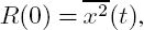
The power spectral density of any signal can be conveniently measured with the help of a selective narrowband power meter tuned across the bandwidth of the signal. The power measured at any frequency is then plotted against the measurement frequency. The autocorrelation function R(τ) of the signal x(t) gives an average indication of how predictable the signal x(t) is after a period of τ seconds from its present value. Accordingly, it is defined as:

(2.2)

For a periodic signal x(t), it is sufficient to evaluate the above equation for a single period T₀, yielding:

(2.3)

The basic properties of the ACF are as follows.

• The ACF is symmetric: R(τ)= R(−τ).
• The ACF is monotonically decreasing: R(τ) ≤ R(0).
• For τ = 0 we have which is the signal’s power.

The ACF and the PSD form a Fourier transform pair. This is formally stated as the Wiener–Khintchine theorem, as follows:

(2.4)

where δ (τ) is the Dirac delta function. Clearly, for any timed-domain shift τ > 0, the noise is uncorrelated.

Bandlimited communications systems bandlimit not only the signal but the noise as well, and this filtering limits the rate of change of the time-domain noise signal, introducing some correlation over the interval of ±1/2B. The stylized PSD and ACF of bandlimited white noise are displayed in Figure 2.4.

After bandlimiting, the autocorrelation function becomes:

(2.5)

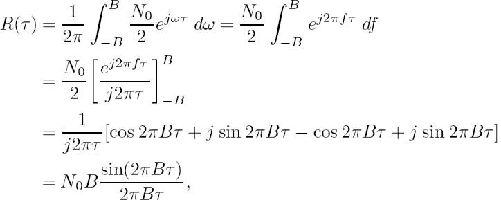
which is the well-known sinc function seen in Figure 2.4.

In the time domain, the amplitude distribution of the white thermal noise has a normal or Gaussian distribution, and since it is inevitably added to the received signal, it is usually referred to as Additive White Gaussian Noise (AWGN). Note that AWGN is therefore the noise generated in the receiver. The Probability Density Function (PDF) is the well-known bell-shaped curve of the Gaussian distribution, given by

(2.6)

where m is the mean and σ² is the variance. The effects of AWGN can be mitigated by increasing the transmitted signal power and thereby reducing the relative effects of noise. The Signal-to-Noise Ratio (SNR) at the receiver’s input provides a good measure of the received signal quality. This SNR is often referred to as the channel SNR.

2.3 Information of a Source

Based on Shannon’s work [133, 215–217, 225, 226], let us introduce the basic terms and definitions of information theory by considering a few simple examples. Assume that a simple eight-bit Analog-to-Digital Converter (ADC) emits a sequence of mutually independent source symbols that can take the values i = 1, 2,. .. , 256 with equal probability. One may wonder how much information can be inferred upon receiving one of these samples. It is intuitively clear that this inferred information is definitely proportional to the ‘uncertainty’ resolved by the reception of one such symbol, which in turn implies that the information conveyed is related to the number of levels in the ADC. More explicitly, the higher the number of legitimate quantization levels, the lower is the relative frequency or probability of receiving any one of them, and hence it is the more ‘surprising’ when any one of them is received. Therefore, less probable quantized samples carry more information than their more frequent, more likely counterparts.

Not surprisingly, one could resolve this uncertainty by simply asking a maximum of 256 questions, such as ‘Is the level 1?,’ ‘Is it 2?’ ... ‘Is it 256?’ Following Hartley’s approach [219], a more efficient strategy would be to ask eight questions, for example: ‘Is the level larger than 128?’ No. ‘Is it larger than 64?’ No ... ‘Is it larger than 2?’ No. ‘Is it larger than 1?’ No. Clearly in this case the source symbol emitted was of magnitude one, provided that the zero level was not a possibility. We can therefore infer that log₂ 256 = 8 ‘Yes/No’ binary answers would be needed to resolve any uncertainty as regards the source symbol’s level.

In more general terms, the information carried by any one symbol of a q-level source, where all the levels are equiprobable with probabilities of p_i = 1/q,i = 1 · · · q, is defined as

(2.7)

Rewriting Equation (2.7) using the message probabilities yields a more convenient form:

(2.8)

which now is also applicable in the case of arbitrary, unequal message probabilities p_i, again implying the plausible fact that the lower the probability of a certain source symbol, the higher the information conveyed by its occurrence. Observe, however, that for unquantized analog sources, where for the number of possible source symbols we have q → ∞, and hence the probability of any analog sample becomes infinitesimally low, these definitions become meaningless.

Let us now consider a sequence of N consecutive q-ary symbols. The number of different values that his sequence can take is q^N, delivering q^N different messages. Therefore, the information carried by one such sequence is:

(2.9)

which is in perfect harmony with our expectation, delivering N times the information of a single symbol, which was quantified by Equation (2.7). Doubling the sequence length to 2N carries twice the information, as suggested by:

(2.10)

Before we proceed, let us briefly summarize the basic properties of information following Shannon’s work [133, 215–217, 225, 226].

• If for the probability of occurrences of the symbols j and k we have p_j < p_k, then as regards the information carried by them we have I(k) < I(j).
• If in the limit we have p_k → 1, then for the information carried by the symbol k we have I(k) → 0, implying that symbols whose probability of occurrence tends to unity carry no information.
• If a symbol’s probability is in the range 0 ≤ p_k ≤ 1, then as regards the information carried by it we have I(k) ≥ 0.
• For independent messages k and j, their joint information is given by the sum of their information: I(k, j) = I(k) + I(j). For example, the information carried by the statement ‘My son is 14 years old and my daughter is 12’ is equivalent to that of the sum of these statements: ‘My son is 14 years old’ and ‘My daughter is 12 years old’.
• In harmony with our expectation, if we have two equiprobable messages 0 and 1 with probabilities p₁ = p₂ = ½, then from Equation (2.8) we have I(0) = I(1) = 1bit.

2.4 Average Information of Discrete Memoryless Sources

Following Shannon’s approach [133,215–217,225,226], let us now consider a source emitting one of q possible symbols from the alphabet s = s₁, s₂, ..., s_i,. .. , s_q having symbol probabilities of p_i, i = 1, 2, ..., q. Suppose that a long message of N symbols constituted by symbols from the alphabet s = s₁, s₂, ..., s_q having symbol probabilities of p_i is to be transmitted. Then the symbol s_i appears in every N-symbol message on average p_i · N number of times, provided the message length is sufficiently long. The information carried by symbol s_i is log ₂1/p_i and its p_i · N occurrences yield an information contribution of

(2.11)

Upon summing the contributions of all the q symbols, we acquire the total information carried by the N-symbol sequence:

(2.12)

Averaging this over the N symbols of the sequence yields the average information per symbol, which is referred to as the source’s entropy [215]:

(2.13)

Then the average source information rate can be defined as the product of the information carried by a source symbol, given by the entropy H and the source emission rate Rs:

(2.14)

Observe that Equation (2.13) is analogous to the discrete form of the first moment, or in other words the mean of a random process with a PDF of p(x), as in

(2.15)

where the averaging corresponds to the integration, and the instantaneous value of the random variable x represents the information log₂ p_i carried by message i, which is weighted by its probability of occurrence p_i quantified for a continuous variable x by p(x).

2.4.1 Maximum Entropy of a Binary Source

Let us assume that a binary source, for which q = 2, emits two symbols with probabilities p₁ = p and p₂ = (1 − p), where the sum of the symbol probabilities must be unity. In order to quantify the maximum average information of a symbol from this source as a function of the symbol probabilities, we note from Equation (2.13) that the entropy is given by:

(2.16)

As in any maximization problem, we set ∂H (p)/∂p = 0, and upon using the differentiation chain rule of (u · v)′ = u′ · v + u · v′ as well as exploiting that (log_a x)′ = 1/x log_a e we arrive at

This result suggests that the entropy is maximal for equiprobable binary messages. Plotting Equation (2.16) for arbitrary p values yields Figure 2.5, in which Shannon suggested that the average information carried by a symbol of a binary source is low if one of the symbols has a high probability while the other has a low probability.

Example: Let us compute the entropy of the binary source having message probabilities of

The entropy is expressed as:

Exploiting the following equivalence:

(2.17)

we have:

again implying that if the symbol probabilities are rather different, the entropy becomes significantly lower than the achievable 1 bit/symbol. This is because the probability of encountering the more likely symbol is so close to unity that it carries hardly any information, which cannot be compensated by the more ‘informative’ symbol’s reception. For the even more unbalanced situation of p₁ = 0.1 and p₂ = 0.9 we have

In the extreme case of p₁ = 0 or p₂ = 1 we have H = 0. As stated before, the average source information rate is defined as the product of the information carried by a source symbol, given by the entropy H and the source emission rate R_s, yielding R = R_s · H [bits/second]. Transmitting the source symbols via a perfect noiseless channel yields the same received sequence without loss of information.

2.4.2 Maximum Entropy of a q-ary Source

For a q-ary source the entropy is given by

(2.18)

where, again, the constraint Σp_i = 1 must be satisfied. When determining the extreme value of the above expression for the entropy H under the constraint of Σp_i = 1, the following term has to be maximized:

(2.19)

where λ is the so-called Lagrange multiplier. Following the standard procedure of maximizing an expression, we set

leading to

which implies that the maximum entropy of a q-ary source is maintained if all message probabilities are identical, although at this stage the value of this constant probability is not explicit. Note, however, that the message probabilities must sum to unity, and hence

(2.20)

Table 2.1: Shannon–Fano Coding Example based on Algorithm 2.1 and Figure 2.6

where a is a constant, leading to a = 1/q = p_i, implying that the entropy of any q-ary source is maximum for equiprobable messages. Furthermore, H is always bounded according to

(2.21)

2.5 Source Coding for a Discrete Memoryless Source

Interpreting Shannon’s work [133, 215–217, 225, 226] further, we see that source coding is the process by which the output of a q-ary information source is converted to a binary sequence for transmission via binary channels, as seen in Figure 2.1. When a discrete memoryless source generates q-ary equiprobable symbols with an average information rate of R = R_s log ₂q, all symbols convey the same amount of information, and efficient signaling takes the form of binary transmissions at a rate of R bits per second. When the symbol probabilities are unequal, the minimum required source rate for distortionless transmission is reduced to

(2.22)

Then the transmission of a highly probable symbol carries little information, and hence assigning log₂ q number of bits to it does not use the channel efficiently. What can be done to improve transmission efficiency? Shannon’s source coding theorem suggests that by using a source encoder before transmission the efficiency of the system with equiprobable source symbols can be arbitrarily approached.

Coding efficiency can be defined as the ratio of the source information rate and the average output bit rate of the source encoder. If this ratio approaches unity, implying that the source encoder’s output rate is close to the source information rate, the source encoder is highly efficient. There are many source encoding algorithms, but the most powerful approach suggested has been Shannon’s method [133], which is best illustrated by means of the example described below and portrayed in Table 2.1, Algorithm 2.1 and Figure 2.6.

2.5.1 Shannon–Fano Coding

The Shannon–Fano coding algorithm is based on the simple concept of encoding frequent messages using short codewords and infrequent ones by long codewords, while reducing the average message length. This algorithm is part of virtually all treatises dealing with information theory, such as, for example, Carlson’s work [221]. The formal coding steps listed in Algorithm 2.1 and in the flowchart of Figure 2.6 can be readily followed in the context of a simple example in Table 2.1. The average codeword length is given by weighting the length of any codeword by its probability, yielding:

Algorithm 2.1 (Shannon–Fano Coding) This algorithm summarizes the Shannon–Fano coding steps. (See also Figure 2.6 and Table 2.1.)

1. The source symbols S0 ... S7 are first sorted in descending order of probability of occurrence. 2. Then the symbols are divided into two subgroups so that the subgroup probabilities are as close to each other as possible. This division is indicated by the horizontal partitioning lines in Table 2.1. 3. When allocating codewords to represent the source symbols, we assign a logical zero to the top subgroup and logical one to the bottom subgroup in the appropriate column under ‘coding steps.’ 4. If there is more than one symbol in the subgroup, this method is continued until no further divisions are possible. 5. Finally, the variable-length codewords are output to the channel.

The entropy of the source is:

(2.23)

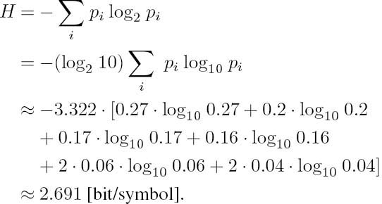
Since the average codeword length of 2.73 bits/symbol is very close to the entropy of 2.691 bit/symbol, a high coding efficiency is predicted, which can be computed as:

The straightforward 3 bits/symbol Binary-Coded Decimal (BCD) assignment gives an efficiency of

In summary, Shannon–Fano coding allowed us to create a set of uniquely invertible mappings to a set of codewords, which facilitate a more efficient transmission of the source symbols than straightforward BCD representations would. This was possible with no coding impairment (i.e., losslessly). Having highlighted the philosophy of the Shannon–Fano noiseless or distortionless coding technique, let us now concentrate on the closely related Huffman coding principle.

2.5.2 Huffman Coding

The Huffman Coding algorithm is best understood by referring to the flowchart in Figure 2.7 and to the formal coding description in Algorithm 2.2. A simple practical example is portrayed in Table 2.2, which leads to the Huffman codes summarized in Table 2.3. Note that we have used the same symbol probabilities as in our Shannon–Fano coding example, but the Huffman algorithm leads to a different codeword assignment. Nonetheless, the code’s efficiency is identical to that of the Shannon–Fano algorithm.

The symbol-merging procedure can also be conveniently viewed using the example of Figure 2.8, where the Huffman codewords are derived by reading the associated 1 and 0 symbols from the end of the tree backwards; that is, towards the source symbols S₀ · · · S₇. Again, these codewords are summarized in Table 2.3.

In order to arrive at a fixed average channel bit rate, which is convenient in many communications systems, a long buffer might be needed, causing storage and delay problems. Observe from Table 2.3 that the Huffman coding algorithm gives codewords that can be uniquely decoded, which is a crucial prerequisite for its practical employment. This is because no codeword can be a prefix of any longer one. For example, for the sequence of codewords ..., 00, 10, 010, 110, 1111, ... the source sequence of ... S₀, S₁, S₂, S₃, S₈ ... can be uniquely inferred from Table 2.3.

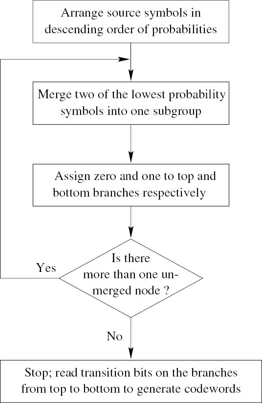
Algorithm 2.2 (Huffman Coding) This algorithm summarizes the Huffman coding steps.

1. Arrange the symbol probabilities pi in decreasing order and consider them as ‘leaf-nodes,’ as suggested by Table 2.2. 2. While there is more than one node, merge the two nodes having the lowest probabilities, and assign 0 and 1 to the upper and lower branches respectively. 3. Read the assigned ‘transition bits’ on the branches from top to bottom in order to derive the codewords.

Table 2.2: Huffman Coding Example Based on Algorithm 2.2 and Figure 2.7 (for final code assignment see Table 2.3)

In our discussions so far, we have assumed that the source symbols were completely independent of each other. Such a source is usually referred to as a memoryless source. By contrast, sources where the probability of a certain symbol also depends on what the previous symbol was are often termed sources exhibiting memory. These sources are typically bandlimited sample sequences, such as, for example, a set of correlated or ‘similar-magnitude’ speech samples or adjacent video pixels. Let us now consider sources that exhibit memory.

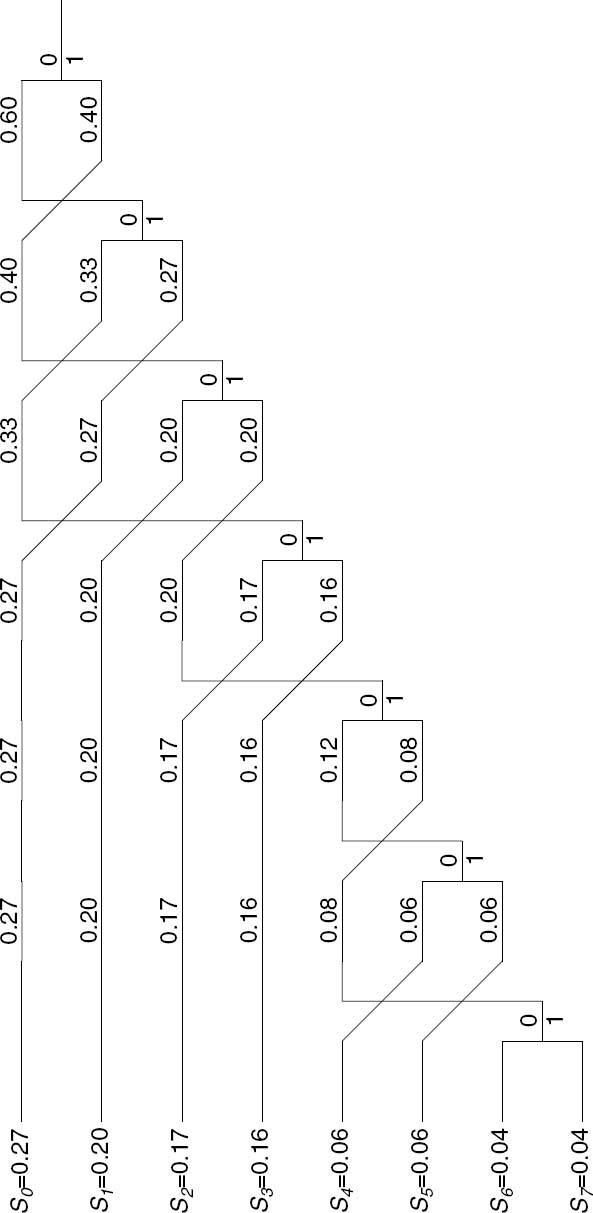
Table 2.3: Huffman Coding Example Summary of Table 2.2

2.6 Entropy of Discrete Sources Exhibiting Memory

Let us invoke Shannon’s approach [133, 215–217, 225, 226] in order to illustrate sources with and without memory. Let us therefore consider an uncorrelated random White Gaussian Noise (WGN) process, which has been passed through a low-pass filter. The corresponding ACFs and Power Spectral Density (PSD) functions were portrayed in Figures 2.3 and 2.4. Observe in the figures that through low-pass filtering a WGN process introduces correlation by limiting the rate at which amplitude changes are possible, smoothing the amplitude of abrupt noise peaks. This example suggests that all bandlimited signals are correlated over a finite interval. Most analog source signals, such as speech and video, are inherently correlated, owing to physical restrictions imposed on the analog source. Hence all practical analog sources possess some grade of memory, a property that is also retained after sampling and quantization. An important feature of sources with memory is that they are predictable to a certain extent; hence, they can usually be more efficiently encoded than unpredictable sources having no memory.

2.6.1 Two-State Markov Model for Discrete Sources Exhibiting Memory

Let us now introduce a simple analytically tractable model for treating sources that exhibit memory. Predictable sources that have memory can be conveniently modeled by Markov processes. A source having a memory of one symbol interval directly ‘remembers’ only the previously emitted source symbol, and it emits one of its legitimate symbols with a certain probability, which depends explicitly on the state associated with this previous symbol. A one-symbol-memory model is often referred to as a first-order model. As an example, if in a first-order model the previous symbol can take only two different values, we have two different states, and this simple two-state first-order Markov model is characterized by the state transition diagram of Figure 2.9. Previously, in the context of Shannon–Fano and Huffman coding of memoryless information sources, we used the notation of S_i, i = 0, 1,.. ., for the various symbols to be encoded. In this section we are dealing with sources exhibiting memory, and hence for the sake of distinction we use the symbol notation of X_i, i = 1, 2, .... If, for the sake of illustration, the previous emitted symbol was X₁, the state machine of Figure 2.9 is in state X₁, and in the current signaling interval it can generate one of two symbols, namely, X₁ and X₂, whose probability depends explicitly on the previous state X₁. However, not all two-state Markov models are as simple as that of Figure 2.9, since the transitions from state X₁ to X₂ are not necessarily associated with emitting the same symbol as the transitions from state X₂ to X₁. A more elaborate example will therefore be considered later in this chapter.

Observe in Figure 2.9 that the corresponding transition probabilities from state X₁ are given by the conditional probabilities p₁₂ = P(X₂/X₁) and p₁₁ = P(X₁/X₁)=1 − P(X₂/X₁). Similar findings can be observed as regards state X₂. These dependencies can also be stated from a different point of view as follows. The probability of occurrence of a particular symbol depends not only on the symbol itself, but also on the previous symbol emitted. Thus, the symbol entropy for states X₁ and X₂ will now be characterized by means of the conditional probabilities associated with the transitions merging in these states. Explicitly, the symbol entropy for state X_i, i = 1, 2 is given by

(2.24)

yielding the symbol entropies (that is, the average information carried by the symbols emitted) in states X₁ and X₂ respectively as

(2.25)

The symbol entropies, H₁ and H₂, are characteristic of the average information conveyed by a symbol emitted in states X₁ and X₂ respectively. In order to compute the overall entropy H of this source, they must be weighted by the probabilities of occurrence, P₁ and P₂, of these states:

(2.26)

Assuming a highly predictable source having high adjacent sample correlation, it is plausible that once the source is in a given state it is more likely to remain in that state than to traverse into the other state. For example, assuming that the state machine of Figure 2.9 is in state X₁ and the source is a highly correlated, predictable one, we are likely to observe long runs of X₁. Conversely, once it is in state X₂, long strings of X₂ symbols will typically follow.

2.6.2 N-State Markov Model for Discrete Sources Exhibiting Memory

In general, assuming N legitimate states, (i.e., N possible source symbols) and following similar arguments, Markov models are characterized by their state probabilities P(X_i), i = 1, ..., N, where N is the number of states, as well as by the transition probabilities p_ij = P(X_i/X_j), where p_ij explicitly indicates the probability of traversing from state X_j to state X_i. Their further basic feature is that they emit a source symbol at every state transition, as shown in the context of an example presented in Section 2.7. Similarly to the two-state model, we define the entropy of a source having memory as the weighted average of the entropy of the individual symbols emitted from each state, where the weighting takes into account the probabilities of occurrence of the individual states, namely P_i. In analytical terms, the symbol entropy for state X_i, i = 1,.. ., N is given by:

(2.27)

The averaged, weighted symbol entropies give the source entropy:

(2.28)

Finally, assuming a source symbol rate of υ_s, the average information emission rate R of the source is given by:

(2.29)

2.7 Examples

2.7.1 Two-State Markov Model Example

As mentioned in the previous section, we now consider a slightly more sophisticated Markov model, where the symbols emitted upon traversing from state X₁ to X₂ are different from those when traversing from state X₂ to X₁.

More explicitly, consider a discrete source that was described by the two-state Markov model of Figure 2.9, where the transition probabilities are

p₁₁ = P(X₁/X₁) = 0.9 p₂₂ = P(X₂/X₂) = 0.1

p₁₂ = P(X₁/X₂) = 0.1 p₂₁ = P(X₂/X₁) = 0.9,

while the state probabilities are

(2.30)

The source emits one of four symbols, namely, a, b, c, and d, upon every state transition, as seen in Figure 2.10. Let us find:

• the source entropy;
• the average information content per symbol in messages of one, two, and three symbols.

Message Probabilities

Let us consider two sample sequences acb and aab. As shown in Figure 2.10, the transitions leading to acb are (1 1), (1 2) and (2 2). The probability of encountering this sequence is 0.8 · 0.9 · 0.1 · 0.1 = 0.0072. The sequence aab has a probability of zero because the transition from a to b is illegal. Further path (i.e., message) probabilities are given in Table 2.4 along with the information I = −log₂ P conveyed by all of the legitimate messages.

Table 2.4: Message probabilities of example

Message probabilities	Information conveyed (bits/message)
Pa = 0.9 × 0.8 = 0.72	Ia = 0.474
Pb = 0.1 × 0.2 = 0.02	Ib = 5.644
Pc = 0.1 × 0.8 = 0.08	Ic = 3.644
Pd = 0.9 × 0.2 = 0.18	Id = 2.474
Paa = 0.72 × 0.9 = 0.648	Iaa = 0.626
Pac = 0.72 × 0.1 = 0.072	Iac = 3.796
Pcb = 0.08 × 0.1 = 0.008	Icb = 6.966
Pcd = 0.08 × 0.9 = 0.072	Icd = 3.796
Pbb = 0.02 × 0.1 = 0.002	Ibb = 8.966
Pbd = 0.02 × 0.9 = 0.018	Ibd = 5.796
Pda = 0.18 × 0.9 = 0.162	Ida = 2.626
Pdc = 0.18 × 0.1 = 0.018	Idc = 5.796

Source Entropy

According to Equation (2.27), the entropies of symbols X₁ and X₂ are computed as

(2.31)

(2.32)

Then their weighted average is calculated using the probability of occurrence of each state in order to derive the average information per message for this source:

The average information per symbol I₂ in two-symbol messages is computed from the entropy h₂ of the two-symbol messages, which is

(2.33)

giving I₂ = h₂/2 ≈ 0.83 bits/symbol information on average when receiving a two-symbol message.

There are eight two-symbol messages; hence, the maximum possible information conveyed is log₂ 8 = 3 bits/2 symbols, or 1.5 bits/symbol. However, since the symbol probabilities of P₁ = 0.8 and P₂ = 0.2 are fairly different, this scheme has a significantly lower conveyed information per symbol, namely I₂ ≈ 0.83 bits/symbol.

Similarly, one can find the average information content per symbol for arbitrarily long messages of concatenated source symbols. For one-symbol messages we have:

(2.34)

We note that the maximum possible information carried by one-symbol messages is h_1max = log₂ 4 = 2 bits/symbol, since there are four one-symbol messages in Table 2.4.

Observe the important tendency in which, when sending longer messages from dependent sources, the average information content per symbol is reduced. This is due to the source’s memory, since consecutive symbol emissions are dependent on previous ones and hence do not carry as much information as independent source symbols would. This becomes explicit by comparing I₁ ≈ 1.191 and I₂ ≈ 0.83 bits/symbol.

Therefore, expanding the message length to be encoded yields more efficient coding schemes, requiring a lower number of bits, if the source has a memory. This is the essence of Shannon’s source coding theorem.

2.7.2 Four-State Markov Model for a Two-Bit Quantizer

Let us now augment the previously introduced two-state Markov model concepts with the aid of a four-state example. Let us assume that we have a discrete source constituted by a two-bit quantizer, which is characterized by Figure 2.11. Assume further that due to bandlimitation only transitions to adjacent quantization intervals are possible, since the bandlimitation restricts the input signal’s rate of change. The probabilities of the signal samples residing in intervals 1–4 are given by

P(1) = P(4) = 0.1, P(2) = P(3) = 0.4.

The associated state transition probabilities are shown in Figure 2.11, along with the quantized samples a, b, c and d, which are transmitted when a state transition takes place – that is, when taking a new sample from the analog source signal at the sampling rate f_s.

Although we have stipulated a number of simplifying assumptions, this example attempts to illustrate the construction of Markov models in the context of a simple practical problem. Next we construct a simpler example for use in augmenting the underlying concepts, and set aside the above four-state Markov model example as a potential exercise for the reader.

2.8 Generating Model Sources

2.8.1 Autoregressive Model

In evaluating the performance of information processing systems such as encoders and predictors, it is necessary to have ‘standardized’ or easily described model sources. Although a set of semi-standardized test sequences of speech and images is widely used in preference to analytical model sources by researchers in codec performance testing, real speech or image sources cannot be used in analytical studies. A widely used analytical model source is the Autoregressive (AR) model. A zero-mean random sequence y(n) is called an AR process of order p if it is generated as follows:

(2.35)

where ε(n) is an uncorrelated zero-mean, random input sequence with variance σ²; that is,

(2.36)

Equation (2.35) states that an AR system recursively generates the present output from p previous output samples given by y(n − k) and the present random input sample ε(n).

2.8.2 AR Model Properties

AR models are very useful in studying information processing systems, such as speech and image codecs, predictors and quantizers. They have the following basic properties:

• The first term of Equation (2.35), which is repeated here for convenience,
  
  defines a predictor, giving an estimate (n) of y(n), which is associated with the minimum mean squared error between the two quantities.
• Although (n) and y(n) depend explicitly only on the past p samples of y(n), through the recursive relationship of Equation (2.35) this entails the entire past of y(n). This is because each of the previous p samples depends on its predecessors.
• Equation (2.35) can therefore be written in the form of

(2.37)

where ε(n) is the prediction error and (n) is the minimum variance prediction estimate of y(n).

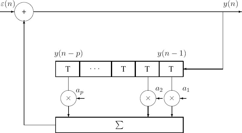
• Without proof, we state that for a random Gaussian distributed prediction error sequence ε(n) these properties are characteristic of a pth order Markov process, as portrayed in Figure 2.12. When this model is simplified for the case of p = 1, we arrive at the schematic diagram shown in Figure 2.13.
• The PSD of the prediction error sequence ε(n) is that of a random ‘white noise’ sequence, containing all possible frequency components with the same energy. Hence, its ACF is the Kronecker delta function, given by the Wiener–Khintchine theorem:

(2.38)

2.8.3 First-Order Markov Model

A variety of practical information sources are adequately modeled by the analytically tractable first-order Markov model depicted in Figure 2.13, where the prediction order is p = 1. With the aid of Equation (2.35) we have

y(n) = ε(n) + ay (n − 1),

where a is the adjacent sample correlation of the process y(n). Using the following recursion:

(2.39)

we arrive at:

which can be generalized to:

(2.40)

Clearly, Equation (2.40) describes the first-order Markov process with the help of the adjacent sample correlation a₁ and the uncorrelated zero-mean random Gaussian process ε(n).

2.9 Run-Length Coding for Discrete Sources Exhibiting Memory

2.9.1 Run-Length Coding Principle [221]

For discrete sources having memory (i.e., possessing intersample correlation), the coding efficiency can be significantly improved by predictive coding, allowing the required transmission rate and hence the channel bandwidth to be reduced. Particularly amenable to run-length coding are binary sources with inherent memory, such as black-and-white documents, where the predominance of white pixels suggests that a Run-Length Coding (RLC) scheme, which encodes the length of zero runs rather than repeating long strings of zeros, provides high coding efficiency.

Following Carlson’s interpretation [221], a predictive RLC scheme can be constructed as shown in Figure 2.14. The q-ary source messages are first converted to binary bit format. For example, if an 8-bit ADC is used, the 8-bit digital samples are converted to binary format. This bit stream, x(i), is then compared with the output signal of the predictor, (i), which is fed with the prediction error signal e(i). The comparator is a simple mod-2 gate, outputting a logical one whenever the prediction fails; that is, the predictor’s output is different from the incoming bit x(i). If, however, x(i) = (i), the comparator indicates this by outputting a logical zero. For highly correlated signals from sources with significant memory the predictions are usually correct, and hence long strings of zero runs are emitted, interspersed with an occasional one. Thus, the prediction error signal e(i) can be efficiently run-length encoded by noting and transmitting the length of zero runs.

The corresponding binary run-length coding principle becomes explicit from Table 2.5 and from our forthcoming coding efficiency analysis.

2.9.2 Run-Length Coding Compression Ratio [227]

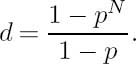
Following Jain’s interpretation [227], let us now investigate the RLC efficiency by assuming that a run of r successive logical zeros is followed by a one. Instead of directly transmitting these strings, we represent such a string as an n-bit word giving the length of the zero run between successive logical ones. When a zero run longer than N = 2ⁿ − 1 bits occurs, this is signaled as the all-ones codeword, informing the decoder to wait for the next RLC codeword before releasing the decoded sequence. The scheme’s operation is characterized by Table 2.5. Clearly, data compression is achieved if the average number of zero data bits per run d is higher than the number of bits, n, required to encode the zero-run length. Let us therefore compute the average number of bits per run without RLC. If a run of r logical

Table 2.5: Run-Length Coding Table © Carlson, 1975 [221]

zeros is followed by a one, the run length is (r + 1). The expected or mean value of (r + 1), namely is calculated by weighting each specific (r + 1) with its probability of occurrence, that is, with its discrete PDF c(r), and then averaging the weighted components:

(2.41)

The PDF of a run of r zeros followed by a one is given by:

(2.42)

since the probability of N consecutive zeros is p^N if r = N, while for shorter runs the joint probability of r zeros followed by a one is given by p^r · (1 − p). The PDF and CDF of this distribution are shown in Figure 2.15 for p = 0.9 and p = 0.1, where p represents the probability of a logical zero bit. Substituting Equation (2.42) in Equation (2.41) gives

(2.43)

Equation (2.43) is a simple geometric progression, given in closed form as

(2.44)

RLC Example: Using a run-length coding memory of M = 31 and a zero symbol probability of p = 0.95, characterize the RLC efficiency.

Substituting N and p into Equation (2.44) for the average run length we have

(2.45)

The compression ratio C achieved by RLC is given by

(2.46)

The achieved average bit rate is

and the coding efficiency is computed as the ratio of the entropy (i.e., of the lowest possible bit rate and the actual bit rate). The source entropy is given by

(2.47)

giving a coding efficiency of

E = H/B ≈ 0.286/0.314 ≈ 91%.

This concludes our RLC example.

2.10 Information Transmission via Discrete Channels

Let us now return to Shannon’s classic references [133, 215–217, 225, 226] and assume that both the channel and the source are discrete, and let us evaluate the amount of information transmitted via the channel. We define the channel capacity characterizing the channel and show that according to Shannon nearly error-free information transmission is possible at rates below the channel capacity via the Binary Symmetric Channel (BSC). Let us begin our discourse with a simple introductory example.

2.10.1 Binary Symmetric Channel Example

Let us assume that a binary source is emitting a logical one with a probability of P(1) = 0.7 and a logical zero with a probability of P(0) = 0.3. The channel’s error probability is p_e = 0.02. This scenario is characterized by the BSC model of Figure 2.16. The probability of error-free reception is given by that of receiving a logical one when a one is transmitted plus the probability of receiving a zero when a zero is transmitted. This is also plausible from Figure 2.16. For example, the first of these two component probabilities can be computed with the aid of Figure 2.16 as the product of the probability P(1) of a logical one being transmitted and the conditional probability P(1/1) of receiving a one, given the condition that a one was transmitted:

(2.48)

Similarly, the probability of the error-free reception of a logical zero is given by

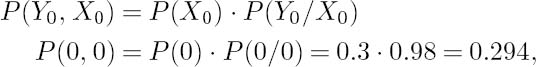
giving the total probability of error-free reception as

Following similar arguments, the probability of erroneous reception is also given by two components. For example, using Figure 2.16, the probability of receiving a one when a zero was transmitted is computed by multiplying the probability P(0) of a logical zero being transmitted by the conditional probability P(1/0) of receiving a logical one, given the fact that a zero is known to have been transmitted:

Conversely,

yielding a total error probability of

which is constituted by the above two possible error events.

Viewing events from a different angle, we observe that the total probability of receiving a one is that of receiving a transmitted one correctly plus that of receiving a transmitted zero incorrectly:

(2.49)

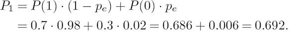
On the same note, the probability of receiving a zero is that of receiving a transmitted zero correctly plus that of receiving a transmitted one incorrectly:

(2.50)

In the next example, we further study the performance of the BSC for a range of different parameters in order to gain a deeper insight into its behavior.

Example: Repeat the above calculations for P(1) = 1,0.9,0.5, and p_e = 0,0.1,0.2,0.5 using the BSC model of Figure 2.16. Compute and tabulate the probabilities P (1,1), P (0,0), P (1,0), P (0,1), P_correct, P_error, P₁ and P₀ for these parameter combinations, including also their values for the previous example, namely for P(1) = 0.7, P(0) = 0.3 and p_e = 0.02. Here we neglect the details of the calculations and summarize the results in Table 2.6. Some of the above quantities are plotted for further study in Figure 2.17, which reveals the interdependency of the various probabilities for the interested reader.

Having studied the performance of the BSC, the next question that arises is how much information can be inferred upon reception of a one and a zero over an imperfect (i.e., error-prone) channel. In order to answer this question, let us first generalize the above intuitive findings in the form of Bayes’s rule.

2.10.2 Bayes’ Rule

Let Y_j represent the received symbols and X_i the transmitted symbols having probabilities of P(Y_j) and P(X_i) respectively. Let us also characterize the forward transition probabilities of the binary symmetric channel as suggested by Figure 2.18.

Then in general, following from the previous introductory example, the joint probability P(Y_j, X_i), of receiving Y_j when the transmitted source symbol was X_i, is computed as the

Table 2.6: BSC Performance Table

probability P(X_i) of transmitting X_i multiplied by the conditional probability P(Y_j/X_i) of receiving Y_j when X_i is known to have been transmitted:

(2.51)

a result that we have already intuitively exploited in the previous example. Since for the joint probabilities P(Y_j, X_i) = P (X_i, Y_j) holds, we have

(2.52)

Equation (2.52) is often presented in the form

(2.53)

which is referred to as Bayes’s rule.

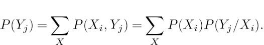
Logically, the probability of receiving a particular Y_j = Y_j0 is the sum of all joint probabilities P(X_i, Y_j0) over the range of X_i. This corresponds to the probability of receiving the transmitted X_i correctly, giving rise to the channel output Y_j0 plus the sum of the probabilities of all other possible transmitted symbols giving rise to Y_j0:

(2.54)

Similarly:

(2.55)

2.10.3 Mutual Information

In this subsection, we elaborate further on the ramifications of Shannon’s information theory [133, 215–217, 225, 226]. Over nonideal channels impairments are introduced, and the received information might be different from the transmitted information. Here we quantify the amount of information that can be inferred from the received symbols over noisy channels. In the spirit of Shannon’s fundamental work [133] and Carlson’s classic reference [221], let us continue our discourse with the definition of mutual information. We have already used the notation P(X_i) to denote the probability that the source symbol X_i was transmitted and P(Y_j) to denote the probability that the symbol Y_j was received. The joint probability that X_i was transmitted and Y_j was received had been quantified by P(X_i, Y_j), and P(X_i/Y_j) indicated the conditional probability that X_i was transmitted, given that Y_j was received, while P(Y_j/X_i) was used for the conditional probability that Y_j was received given that X_i was transmitted.

In the case of i = j, the conditional probabilities P(Y_j/X_j)j = 1 · · · q represent the error-free transmission probabilities of the source symbols j = 1 · · · q. For example, in Figure 2.18 the probabilities P(Y₀/X₀) and P(Y₁/X₁) are the probabilities of the error-free reception of a transmitted X₀ and X₁ source symbol, respectively. The probabilities P(Y_j/X_i)j ≠ i on the other hand, give the individual error probabilities, which are characteristic of error events that corrupted a transmitted symbol X_i to a received symbol Y_j. The corresponding error probabilities in Figure 2.18 are P(Y₀/X₁) and P(Y₁/X₀).

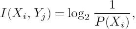
Let us define the mutual information of X_i and Y_j as

(2.56)

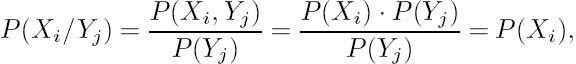
which quantifies the amount of information conveyed when X_i is transmitted and Y_j is received. Over a perfect, noiseless channel, each received symbol Y_j uniquely identifies a transmitted symbol X_i with a probability of P(X_i/Y_j) = 1. Substituting this probability in Equation (2.56) yields a mutual information of

(2.57)

which is identical to the self-information of X_i; hence no information is lost over the channel. If the channel is very noisy and the error probability becomes 0.5, then the received symbol Y_j becomes unrelated to the transmitted symbol X_i, since for a binary system upon its reception there is a probability of 0.5 that X₀ was transmitted and the probability of X₁ is also 0.5. Then formally X_i and Y_j are independent, and hence

(2.58)

giving a mutual information of

(2.59)

implying that no information is conveyed via the channel. Practical communications channels perform between these extreme values and are usually characterized by the average mutual information, defined as

(2.60)

Clearly, the average mutual information in Equation (2.60) is computed by weighting each component I(X_i, Y_j) by its probability of occurrence P(X_i, Y_j) and summing these contributions for all combinations of X_i and Y_j. The average mutual information I(X, Y) defined above gives the average amount of source information acquired per received symbol, as distinguished from that per source symbol, which was given by the entropy H(X). Let us now consolidate these definitions by working through the following numerical example.

2.10.4 Mutual Information Example

Using the same numeric values as in our introductory example of the binary symmetric channel in Section 2.10.1, and exploiting Bayes’s rule as given in Equation (2.53), we have

The following probabilities can be derived, which will be used at a later stage in order to determine the mutual information:

and

where P₁ = 0.692 and P₀ = 0.3080 represent the total probabilities of receiving a one and a zero respectively, which are the unions of the respective events of error-free and erroneous receptions yielding the specific logical value concerned. The mutual information from Equation (2.56) is computed as

(2.61)

(2.62)

These figures must be contrasted with the amount of source information conveyed by the source symbols X₀ and X₁:

(2.63)

and

(2.64)

The amount of information ‘lost’ in the noisy channel is given by the difference between the amount of information carried by the source symbols and the mutual information gained upon inferring a particular symbol at the noisy channel’s output. Hence the lost information can be computed from Equations (2.61), (2.62), (2.63) and (2.64), yielding (1.737 − 1.67) ≈ 0.067 bits and (0.5146 − 0.502) ≈ 0.013 bits respectively. These values may not seem catastrophic, but in relative terms they are quite substantial and their values rapidly escalate as the channel error probability is increased. For the sake of completeness and for future use, let us compute the remaining mutual information terms, namely I(X₀, Y₁) and I(X₁, Y₀), which necessitate the computation of

(2.65)

(2.66)

where the negative sign reflects the amount of ‘misinformation’ as regards, for example, X₀ upon receiving Y₁. In this example we informally introduced the definition of mutual information. Let us now set out to formally exploit the benefits of our deeper insight into the effects of the noisy channel.

2.10.5 Information Loss via Imperfect Channels

Upon rewriting the definition of mutual information in Equation (2.56), we have

(2.67)

Following Shannon’s [133,215–217,225,226] and Ferenczy’s [223] approach and rearranging Equation (2.67) yields

(2.68)

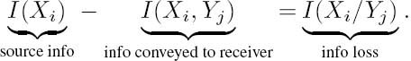
Briefly returning to Figure 2.18 assists the interpretation of P(X_i/Y_j) as the probability, or the degree of certainty, or in fact uncertainty, associated with the event that X_i was transmitted given that Y_j was received, which justifies the above definition of the information loss. It is useful to observe from this figure that, as was stated before, P(Y_j/X_i) represents the probability of erroneous or error-free reception. Explicitly, if j = i, then P(Y_j/X_i) = P(Y_j/X_j) is the probability of error-free reception, while if j ≠ i, then P(Y_j/X_i) is the probability of erroneous reception.

With the probability P(Y_j/X_i) of erroneous reception in mind, we can actually associate an error information term with it:

(2.69)

Let us now concentrate on the expression for average mutual information in Equation (2.60), and expand it as follows:

(2.70)

Considering the first term on the right-hand side (rhs) of the above equation and invoking Equation (2.55), we have

(2.71)

Then rearranging Equation (2.70) gives

(2.72)

where H(X) is the average source information per symbol and I(X, Y) is the average conveyed information per received symbol.

Consequently, the rhs term must be the average information per symbol lost in the noisy channel. As we have seen in Equations (2.67) and (2.68), the information loss is given by

(2.73)

The average information loss H(X/ Y), which Shannon [216] terms equivocation, is computed as the weighted sum of these components:

(2.74)

Following Shannon, this definition allows us to express Equation (2.72) as:

(2.75)

2.10.6 Error Entropy via Imperfect Channels

Similarly to our previous approach and using the probability P(Y_j/X_i) of erroneous reception associated with the information term of

(2.76)

we can define the average ‘error information’ or error entropy. Hence the above error information terms (Equation (2.76)) are weighted using the probabilities P(X_i,Y_j) and averaged for all X and Y values, defining the error entropy:

(2.77)

Using Bayes’s rule from Equation (2.52), we have

(2.78)

Following from this, for the average mutual information in Equation (2.56) we have

(2.79)

which, after interchanging X and Y in Equation (2.75), gives

(2.80)

Subtracting the conveyed information from the destination entropy gives the error entropy, which is nonzero if the destination entropy and the conveyed information are unequal due to channel errors. Let us now proceed following Ferenczy’s approach [223] and summarize the most important definitions for future reference in Table 2.7 before we attempt to augment their physical interpretations using the forthcoming numerical example.

Example: Using the BSC model of Figure 2.16, as an extension of the worked examples of Subsections 2.10.1 and 2.10.4 and following Ferenczy’s interpretation [223] of Shannon’s elaborations [133, 215–217, 225, 226], let us compute the following range of system characteristics:

(a) The joint information, as distinct from the mutual information introduced earlier, for all possible channel input/output combinations.

(b) The entropy, i.e., the average information of both the source and the sink.

(c) The average joint information H(X, Y).

(d) The average mutual information per symbol conveyed.

(e) The average information loss and average error entropy.

With reference to Figure 2.16 and to our introductory example from Section 2.10.1 we commence by computing further parameters of the BSC. Recall that the source information

Table 2.7: Summary of Definitions © Ferenczy [223]

was

The probability of receiving a logical zero was 0.308 and that of a logical one was 0.692, whether zero or one was transmitted. Hence, the information inferred upon the reception of zero and one, respectively, is given by

Observe that because of the reduced probability of receiving a logical one from 0.7 → 0.692 as a consequence of channel-induced corruption, the probability of receiving a logical zero is increased from 0.3 → 0.308. This is expected to increase the average destination entropy, since the entropy maximum of unity is achieved, when the symbols are equiprobable. We note, however, that this does not give more information about the source symbols, which must be maximized in an efficient communications system. In our example, the information conveyed increases for the reduced probability logical one from 0.515 bits → 0.531 bits and decreases for the increased probability zero from 1.737 bits → 1.699 bits. Furthermore, the average information conveyed is reduced, since the reduction from 1.737 to 1.699 bits is more than the increment from 0.515 to 0.531. In the extreme case of an error probability of 0.5 we would have P(0) = P(1) = 0.5, and I(1) = I(0) = 1 bit, associated with receiving equiprobable random bits, which again would have a maximal destination entropy, but minimal information concerning the source symbols transmitted. Following the above interesting introductory calculations, let us now turn our attention to the computation of the joint information.

(a) The joint information, as distinct from the mutual information introduced earlier in Equation (2.56), of all possible channel input/output combinations is computed from Figure 2.16 as follows

(2.81)

These information terms can be individually interpreted formally as the information carried by the simultaneous occurrence of the given symbol combinations. For example, as it accrues from their computation, I₀₀ and I₁₁ correspond to the favorable event of error-free reception of a transmitted zero and one respectively, which hence were simply computed by formally evaluating the information terms. By the same token, in the computation of I₀₁ and I₁₀, the corresponding source probabilities were weighted by the channel error probability rather than the error-free transmission probability, leading to the corresponding information terms. The latter terms, namely I₀₁ and I₁₀, represent low-probability, high-information events due to the low channel error probability of 0.02.

Lastly, a perfect channel with zero error probability would render the probability of the error events zero, which in turn would assign infinite information contents to the corresponding terms of I₀₁ and I₁₀, while I₀₀ and I₁₁ would be identical to the self-information of the zero and one symbols. Then, if under zero error probability we evaluate the effect of the individual symbol probabilities on the remaining joint information terms, the less frequently a symbol is emitted by the source the higher its associated joint information term becomes, and vice versa, which is seen by comparing I₀₀ and I₁₁. Their difference can be equalized by assuming an identical probability of 0.5 for both, which would yield I₀₀ = I₁₁ = 1 bit. The unweighted average of I₀₀ and I₁₁ would then be lower than in the case of the previously used probabilities of 0.3 and 0.7 respectively, since the maximum average would be associated with the case of zero and one, where the associated log₂terms would be 0 and − ∞, respectively. The appropriately weighted average joint information terms are evaluated under paragraph (c) during our later calculations. Let us now move on to evaluate the average information of the source and the sink.

(b) Calculating the entropy, that is, the average information for both the source and the sink, is quite straightforward and ensues as follows

(2.82)

For the computation of the sink’s entropy, we invoke Equations (2.49) and (2.50), yielding

(2.83)

Again, the destination entropy H(Y) is higher than the source entropy H(X) due to the more random reception caused by channel errors, approaching H(Y) = 1 bit/symbol for a channel bit error rate of 0.5. Note, however, that unfortunately this increased destination entropy does not convey more information about the source itself.

(c) Computing the average joint information H (X, Y) gives

(2.84)

Upon substituting the I_{Xi, Yj} values calculated in Equation (2.81) into Equation (2.84), we have

In order to interpret H(X, Y), let us again scrutinize the definition given in Equation (2.84), which weights the joint information terms of Equation (2.81) by their probability of occurrence. We have argued before that the joint information terms corresponding to erroneous events are high due to the low error probability of 0.02. Observe, therefore, that these high-information symbol combinations are weighted by their low probability of occurrence, causing H(X, Y) to become relatively low. It is also instructive to consider the above terms in Equation (2.84) for the extreme cases of zero and 0.5 error probabilities and for different source emission probabilities, which are left for the reader to explore. Here we proceed considering the average conveyed mutual information per symbol.

(d) The average conveyed mutual information per symbol was defined in Equation (2.60) in order to quantify the average source information acquired per received symbol, and is repeated here for convenience:

Using the individual mutual information terms from Equations (2.61)–(2.66) in Section 2.10.4, we get the average mutual information representing the average amount of source information acquired from the received symbols:

(2.85)

In order to interpret the concept of mutual information, in Section 2.10.4 we noted that the amount of information ‘lost’ owing to channel errors was given by the difference between the amount of information carried by the source symbols and the mutual information gained upon inferring a particular symbol at the noisy channel’s output. These were given in Equations (2.61)–(2.64), yielding (1.737 − 1.67) ≈ 0.067 bits and (0.5146 − 0.502) ≈ 0.013 bits, for the transmission of a zero and a one respectively. We also noted that the negative sign of the terms corresponding to the error events reflected the amount of misinformation as regards, for example, X₀ upon receiving Y₁. Over a perfect channel, the cross-coupling transitions of Figure 2.16 are eliminated, since the associated error probabilities are zero, and hence there is no information loss over the channel. Consequently, the error-free mutual information terms become identical to the self-information of the source symbols, since exactly the same amount of information can be inferred upon reception of a symbol as is carried by its appearance at the output of the source.

It is also instructive to study the effect of different error probabilities and source symbol probabilities in the average mutual information definition of Equation (2.84) in order to acquire a better understanding of its physical interpretation and quantitative power as regards the system’s performance. It is interesting to note, for example, that assuming an error probability of zero will therefore result in average mutual information, which is identical to the source and destination entropy computed above under paragraph (b). It is also plausible that I(X, Y) will be higher than the previously computed 0.7495 bits/symbol if the symbol probabilities are closer to 0.5, or in general in the case of q-ary sources closer to 1/q. As expected, for a binary symbol probability of 0.5 and error probability of zero, we have I(X, Y) = 1 bit/symbol.

(e) Lastly, let us determine the average information loss and average error entropy, which were defined in Equations (2.74) and (2.80) and are repeated here for convenience. Again, we will be using some of the previously computed probabilities from Sections 2.10.1 and 2.10.4, beginning with computation of the average information loss of Equation (2.74):

In order to augment the physical interpretation of the above expression for average information loss, let us examine the main contributing factors in it. It is expected to decrease as the error probability decreases. Although it is not straightforward to infer the clear effect of any individual parameter in the equation, experience shows that as the error probability increases the two middle terms corresponding to the error events become more dominant. Again, the reader may find it instructive to alter some of the parameters on a one-by-one basis and study the way each one’s influence manifests itself in terms of the overall information loss.

Moving on to the computation of the average error entropy, we find its definition equation repeated below, and on inspecting Figure 2.16 we have

The average error entropy in the above expression is expected to fall as the error probability is reduced and vice versa. Substituting different values into its definition equation further augments its practical interpretation. Using our previous results in this section, we see that the average loss of information per symbol, or equivocation, denoted by H(X/Y) is given by the difference between the source entropy of Equation (2.82) and the average mutual information of Equation (2.85), yielding:

H (X/Y) = H(X) − I (X, Y) ≈ 0.8816 −0.7495 ≈ 0.132 bits/symbol,

which, according to Equation (2.75), is identical to the value of H(X/Y) computed earlier. In harmony with Equation (2.80), the error entropy can also be computed as the difference of the average entropy H(Y) in Equation (2.83) of the received symbols and the mutual information I(X, Y) of Equation (2.85), yielding

H (Y) − I(X, Y) ≈ 0.8909 − 0.7495 ≈ 0.141 bits/symbol,

as seen above for H(Y/X).

Having defined the fundamental parameters summarized in Table 2.7 and used in the information-theoretical characterization of communications systems, let us now embark on the definition of channel capacity. Initially, we consider discrete noiseless channels, leading to a brief discussion of noisy discrete channels, and then we proceed to analog channels before exploring the fundamental message of the Shannon–Hartley law.

2.11 Capacity of Discrete Channels [216, 223]

Shannon [216] defined the channel capacity C of a channel as the maximum achievable information transmission rate at which error-free transmission can be maintained over the channel.

Every practical channel is noisy, but by transmitting at a sufficiently high power the channel error probability p_e can be kept arbitrarily low, providing us with a simple initial channel model for our further elaborations. Following Ferenczy’s approach [223], assume that the transmission of symbol X_i requires a time interval of t_i, during which an average of

(2.86)

information is transmitted, where q is the size of the source alphabet used. This approach assumes that a variable-length coding algorithm, such as the previously described Shannon–Fano or the Huffman coding algorithm, may be used in order to reduce the transmission rate to as low as the source entropy. Then the average time required for the transmission of a source symbol is computed by weighting t_i with the probability of occurrence of symbol X_i, i = 1 ...q:

(2.87)

Now we can compute the average information transmission rate υ by dividing the average information content of a symbol by the average time required for its transmission:

(2.88)

The maximum transmission rate υ as a function of the symbol probability P(X_i) must be found. This is not always an easy task, but a simple case occurs when the symbol duration is constant; that is, we have t_i = t₀ for all symbols. Then the maximum of υ is a function of P(X_i) only and we have shown earlier that the entropy H(X) is maximized by equiprobable source symbols, where Then from Equations (2.86) and (2.87) we have an expression for the channel’s maximum capacity:

(2.89)

Shannon [216] characterized the capacity of discrete noisy channels using the previously defined mutual information, describing the amount of average conveyed information, given by

(2.90)

where H(Y) is the average amount of information per symbol at the channel’s output, while H(Y/X) is the error entropy. Here a unity symbol-rate was assumed for the sake of simplicity. Hence, useful information is only transmitted via the channel if H(Y) > H(Y/X). Via a channel with p_e = 0.5, where communication breaks down we have H(Y) = H(Y/X), and the information conveyed becomes I(X, Y) = 0. The amount of information conveyed is maximum if the error entropy H(Y/X) = 0. Therefore, Shannon [216] defined the noisy channel’s capacity as the maximum value of the conveyed information I(X, Y):

(2.91)

where the maximization of Equation (2.91) is achieved by maximizing the first term and minimizing the second term.

In general, the maximization of Equation (2.91) is an arduous task, but for the BSC seen in Figure 2.19 it becomes fairly simple. Let us consider this simple case and assume that the source probabilities of zero and one are P(0) = P(1) = 0.5 and the error probability is p_e. The entropy at the destination is computed as

while the error entropy is given by

(2.92)

In order to be able to compute the capacity of the BSC as a function of the channel’s error probability, let us substitute the required joint probabilities

(2.93)

and the conditional probabilities

(2.94)

into Equation (2.92), yielding

(2.95)

Finally, upon substituting H(Y) and H(Y/X) from above into Equation (2.91), the BSC’s channel capacity becomes

(2.96)

Following Ferenczy’s [223] interpretation of Shannon’s lessons [133,215–217,225,226], the graphic representation of the BSC’s capacity is depicted in Figure 2.20 using various p_e error probabilities.

Observe, for example, that for p_e = 10⁻² the channel capacity is C ≈ 0.9 bits/symbol (that is, close to its maximum of C = 1 bit/symbol), but for higher p_e values it rapidly decays, falling to C = 0.5 bits/symbol around p_e = 10⁻¹. If p_e = 0.5, we have C = 0 bits/symbol; since no useful information transmission takes place, the channel delivers random bits. Notice also that if P(0) ≠ 1 ≠ P(1) = 0.5, then H(Y) < 1 bit/symbol and hence C < C_max = 1 bit/symbol, even if p_e = 0.

2.12 Shannon’s Channel Coding Theorem [220, 228]

In the previous section we derived a simple expression for the capacity of the noisy BSC in Equation (2.96), which was depicted in Figure 2.20 as a function of the channel’s error probability pe. In this section we focus on Shannon’s channel coding theorem, which states that as long as the information transmission rate does not exceed the channel’s capacity, the bit error rate can be kept arbitrarily low [225, 226]. In the context of the BSC channel capacity curve of Figure 2.20, this theorem implies that noise over the channel does not preclude the reliable transmission of information; it only limits the rate at which transmission can take place. Implicitly, this theorem prophesies the existence of an appropriate error correction code, which adds redundancy to the original information symbols. This reduces the system’s useful information throughput but simultaneously allows error correction coding. Instead of providing a rigorous proof of this theorem, we will follow the approach suggested by Abramson [220], which was also used by Hey and Allen [228] in their compilation of Feynman’s lectures, and make it plausible.

The theorem is stated more formally as follows. Let us assume that a message of K useful information symbols is transmitted by assigning it to an N-symbol so-called block code, where the symbols are binary and the error probability is p_e. Then, according to Shannon, upon reducing the coding rate beyond every limit, the error probability obeys the following relationship:

(2.97)

As Figure 2.20 shows, upon increasing the bit error rate p_e, the channel capacity reduces gradually toward zero, which forces the channel coding rate to zero in the limit. This inequality therefore implies that an arbitrarily low BER is possible only when the coding rate R tends to zero, which assumes an infinite-length block code and an infinite coding delay. By scrutinizing Figure 2.20 we can infer that, for example, for a BER of 10⁻¹ an approximately so-called half-rate code is required in order to achieve asymptotically perfect communications, while for a BER of 10⁻² an approximately R ≈ 0.9 code is required.

Shannon’s channel coding theorem does not specify how to create error correction codes that can achieve this predicted performance; it merely states their existence. Hence the error correction coding community has endeavored over the years to create such good codes, but until 1993 it had only limited success. Then in that year Berrou et al. [229] invented the family of iteratively decoded turbo codes, which are capable of approaching the Shannonian predictions within a fraction of a dB.

Returning to the channel coding theorem, Hey and Feynman [228] offered a witty approach to deepening the physical interpretation of this theorem, which we briefly highlight below. Assuming that the block-coded sequences are long, in each block on the average there are t = p_e · N number of errors. In general, t number of errors can be allocated over the block of N positions in

different ways, which are associated with the same number of error patterns. The number of additional parity bits added during the coding process is P = (N − K), which must be sufficiently high for identifying all the C^t_N number of error patterns, in order to allow for inverting (i.e., correcting) the corrupted bits in the required positions. Hence we have [228]

(2.98)

Upon exploiting the Stirling formula of

and taking the logarithm of both sides, we have

Furthermore, when N is large, the first and second terms are diminishingly small in comparison with the last two terms. Thus we have

log_e N! ≈ N log_e N − N.

Then, after taking the logarithm, the factorial expression on the left-hand side (L) of Equation (2.98) can be written as:

L ≈ [N log_e N − N] − [t log_e t − t] − [(N − t) log_e(N − t) − (N − t)].

Now taking into account that t ≈ p_e · N, we have [228]

If we consider that log_e a = log₂a · log_e2, then we can convert the log_e terms to log₂ as follows [228]:

L ≈ N log_e2 [−p_e log₂ p_e − (1 − p_e) log₂(1 − p_e)].

Finally, upon equating this term with the logarithm of the right-hand-side expression of Equation (2.98), we arrive at:

N log_e 2[−p_e log₂ p_e − (1 − p_e) log₂(1 − p_e)] ≤ (N − K) log_e 2,

which can be simplified to

or to a form identical to Equation (2.97):

2.13 Capacity of Continuous Channels [217, 223]

During our previous discussions, it was assumed that the source emitted discrete messages with certain finite probabilities, which would be exemplified by an eight-bit analog-to-digital converter emitting one of 256 discrete values with a certain probability. However, after digital source encoding and channel encoding according to the basic schematic of Figure 2.1 the modulator typically converts the digital messages to a finite set of bandlimited analog waveforms, which are chosen for maximum ‘transmission convenience.’ In this context, transmission convenience can imply a range of issues, depending on the communications channel. Two typical constraints are found with channels that are predominantly either power limited or bandwidth limited, although in many practical scenarios both of these constraints become important. Because of their limited solar power supply, satellite channels tend to be more severely power limited than bandlimited, while typically the reverse situation is experienced in mobile radio systems.

The third part of Shannon’s pioneering paper [217] considers many of these issues. Thus, in what follows we define the measure of information for continuous signals, introduce a concept for the continuous channel capacity, and reveal the relationships among channel bandwidth, channel capacity and channel signal-to-noise ratio, as stated by the Shannon–Hartley theorem. Finally, the ideal communications system transpiring from Shannon’s pioneering work is characterized, before we conclude with a brief discussion of the ramifications of wireless channels as regards the applicability of Shannon’s results.

Let us now assume that the channel’s analog input signal x(t) is bandlimited and hence that it is fully characterized by its Nyquist samples and by its Probability Density Function (PDF) p(x). The analogy of this continuous PDF and that of a discrete source are characterized by P(X_i) ≈ p(X_i)ΔX, which reflects the practical way of experimentally determining the histogram of a bandlimited analog signal by observing the relative frequency of events, when its amplitude resides in a ΔX wide amplitude bin, centered around X_i. As an analogy to the discrete average information or entropy expression of

(2.99)

Shannon [217] introduced the entropy of analog sources, as also noted and exploited, for example, by Ferenczy [223], as

(2.100)

For our previously used discrete sources, we have shown that the source entropy is maximized for equiprobable messages. The question that arises is whether this is also true for continuous PDFs. Shannon [217] derived the maximum of the analog signal’s entropy under the constraints of

(2.101)

(2.102)

based on the calculus of variations. He showed that the entropy of a signal x(t) having a constant variance of σ_x² is maximum, if x(t) has a Gaussian distribution given by

(2.103)

Then the maximum of the entropy can be derived upon substituting this PDF into the expression of the entropy. Let us first take the natural logarithm of both sides of the PDF and convert it to a base two logarithm by taking into account that log_e a = log₂ a · log_e 2, in order to be able to use it in the entropy’s log₂ expression. Then the PDF of Equation (2.103) can be written as

(2.104)

and upon exploiting the fact that log_e 2 = 1/log₂ e, the entropy is expressed according to Shannon [217] and Ferenczy [223] as

(2.105)

Since the maximum of the entropy is proportional to the logarithm of the signal’s average power S_x = σ_x², upon quadrupling the signal’s power the entropy is increased by one bit because the range of uncertainty as regards where the signal samples can reside is expanded.

We are now ready to formulate the channel capacity versus channel bandwidth and versus channel SNR relationship of analog channels. Let us assume white, additive, signal-independent noise with a power of N via the channel. Then the received (signal + noise) power is given by

(2.106)

By the same argument, the channel’s output entropy is maximum if its output signal y(t) has a Gaussian PDF, and its value is computed from Equation (2.105) as

(2.107)

We proceed by taking into account the channel impairments, reducing the amount of information conveyed by the amount of the error entropy H(y/x), giving

(2.108)

where again the noise is assumed to be Gaussian, and hence

(2.109)

Upon substituting Equation (2.107) and Equation (2.109) in Equation (2.108), we have

(2.110)

where, again, both the channel’s output signal and the noise are assumed to have Gaussian distribution.

The analog channel’s capacity is then calculated upon multiplying the information conveyed per source sample by the Nyquist sampling rate of f_s = 2 · f_B, yielding [225]

(2.111)

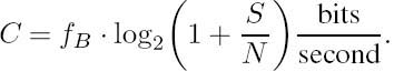
Equation (2.111) is the well-known Shannon–Hartley law,¹ establishing the relationship among the channel capacity C, channel bandwidth f_B and channel Signal-to-Noise Ratio (SNR).

Before analyzing the consequences of the Shannon–Hartley law following Shannon’s deliberations [225], we make it plausible from a simple practical point of view. As we have seen, the Root Mean Squared (RMS) value of the noise is , and that of the signal plus noise at the channel’s output is The receiver has to decide from the noisy channel’s output signal what signal has been input to the channel, although this has been corrupted by an additive Gaussian noise sample. Over an ideal noiseless channel, the receiver would be able to identify what signal sample was input to the receiver. However, over noisy channels it is of no practical benefit to identify the corrupted received message exactly. It is more beneficial to quantify a discretized version of it using a set of decision threshold values, where the resolution is dependent on how corrupted the samples are. In order to quantify this SNR-dependent receiver dynamic range resolution, let us consider the following argument.

Having very densely spaced receiver detection levels would often yield noise-induced decision errors, while a decision-level spacing of according to the RMS noise-amplitude intuitively seems a good compromise between high information resolution and low decision error rate. Then assuming a transmitted sample, which resides at the center of a wide decision interval, noise samples larger than will carry samples across the adjacent decision boundaries. According to this spacing, the number of receiver reconstruction levels is given by

(2.112)

which creates a scenario similar to the transmission of equiprobable q-ary discrete symbols via a discrete noisy channel, each conveying log₂ q amount of information at the Nyquist

sampling rate of f_s = 2 · f_B. Therefore, the channel capacity becomes [225]

(2.113)

as seen earlier in Equation (2.111).

2.13.1 Practical Evaluation of the Shannon–Hartley Law

The Shannon–Hartley law of Equations (2.111) and (2.113) reveals the fundamental relationship of the SNR, bandwidth and channel capacity. This relationship can be further studied, following Ferenczy’s interpretation [223], with reference to Figure 2.21.

Observe from the figure that a constant channel capacity can be maintained, even when the bandwidth is reduced, if a sufficiently high SNR can be guaranteed. For example, from Figure 2.21 we infer that at f_B = 10 KHz and SNR = 30 dB the channel capacity is as high as C = 100 kbits/second. Surprisingly, C ≈ 100 kbits/second can be achieved even for f_B = 5 KHz, if SNR = 60 dB is guaranteed.

Figure 2.22 provides an alternative way of viewing the Shannon–Hartley law, where the SNR is plotted as a function of f_B, parameterized with the channel capacity C. It is important to notice how dramatically the SNR must be increased in order to maintain a constant channel capacity C, as the bandwidth f_B is reduced below 0.1 · C, where C and f_B are expressed in kbits/second and Hz respectively. This is due to the log₂(1 + SNR) function in Equation (2.111), where a logarithmically increasing SNR value is necessitated to compensate for the linear reduction in terms of f_B.

From our previous discourse, the relationship between the relative channel capacity C/f_B, obtained from Equation (2.113), and the channel SNR now becomes plausible.

Table 2.8: Relative channel capacity versus SNR

SNR		C/fB
Ratio	dB	bps/Hz
1	0	1
3	4.8	2
7	8.5	3
15	11.8	4
31	14.9	5
63	18.0	6
127	21.0	7

This relationship is quantified in Table 2.8 and Figure 2.23 for convenience. Notice that due to the logarithmic SNR scale expressed in dB, the curve becomes near-linear, Hz allowing a near-linearly proportional relative channel capacity improvement upon increasing the channel SNR. A very important consequence of this relationship is that if the channel SNR is sufficiently high to support communications using a high number of modulation levels, the channel is not exploited to its full capacity upon using C/f B values lower than are afforded by the prevailing SNR. Proposing various techniques in order to exploit this philosophy was the motivation of [230].

The capacity C of a noiseless channel with SN R = ∞ is C = ∞, although noiseless channels do not exist. In contrast, the capacity of an ideal system with f_B = ∞ is finite [221, 224]. Assuming Additive White Gaussian Noise (AWGN) with a double-sided PSD of η/2, we have and applying the Shannon–Hartley law gives [221]

(2.114)

Our aim is now to determine C_∞ = lim_fB→∞ C. Upon exploiting the fact that

(2.115)

where x = S/(η · f_B), we have

(2.116)

which is the capacity of the channel with f_B = ∞. The practically achievable transmission rate R is typically less than the channel capacity C, although complex turbo-coded modems [229] can approach its value. For example, for a telephone channel with a signal-to-noise ratio of S/N = 10³ = 30 dB and a bandwidth of B = 3.4 kHz from Equation (2.113), we have C = 3.4 · log₂(1 + 10³) kbit/s ≈ 3.4 · 10 = 34 kbit/s, which is fairly close to the rate of the V.34 CCITT standard 28.8 kbit/s telephone-channel modem that was recently standardized.

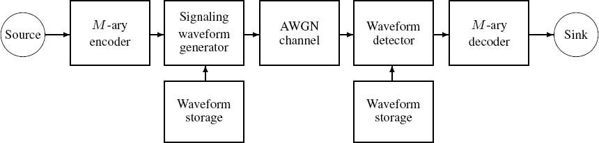
In this chapter we have been concerned with various individual aspects of Shannon’s information theory [133,215–217,225,226]. Drawing nearer to concluding our discourse on the foundations of information theory, let us now outline in broad terms the main ramifications of Shannon’s work [133, 215–217].

2.13.2 Shannon’s Ideal Communications System for Gaussian Channels

The ideal Shannonian communications system shown in Figure 2.24 has the following characteristics. The system’s information-carrying capacity is given by the information rate C = f_B log₂(1 + S/N), while as regards its error rate we have p_e → 0. The transmitted and received signals are bandlimited Gaussian random variables, which facilitate communicating at the highest possible rate over the channel.

Information from the source is observed for T seconds, where T is the symbol duration, and encoded as equiprobable M-ary symbols with a rate of Accordingly, the signaling waveform generator of Figure 2.24 assigns a bandlimited AWGN representation having a maximum frequency of f_B from the set of M = 2^RT possible waveforms to the source message, uniquely representing the signal x(t) to be transmitted for a duration of T. The noisy received signal y(t) = x(t) + n(t) is compared with all M = 2^RT prestored waveforms at the receiver, and the most ‘similar’ is chosen to identify the most likely transmitted source message. The observation intervals at both the encoder and the decoder amount to T, yielding an overall coding delay of 2T. Signaling at a rate equal to the channel capacity is only possible if the source signal’s observation interval is infinitely long, that is, T → ∞.

Before concluding this chapter we offer a brief discussion of the system-architectural ramifications of transmitting over wireless channels rather than over AWGN channels.

2.14 Shannon’s Message for Wireless Channels

In wireless communications over power-and bandlimited channels it is always of prime concern to maintain an optimum compromise in terms of the contradictory requirements of low bit rate, high robustness against channel errors, low delay and low complexity. The minimum bit rate at which distortionless communication is possible is determined by the entropy of the speech source message. Note, however, that in practical terms the source rate corresponding to the entropy is only asymptotically achievable as the encoding memory length or delay tends to infinity. Any further compression is associated with information loss or coding distortion. Note that the optimum source encoder generates a perfectly uncorrelated source-coded stream, where all the source redundancy has been removed; therefore, the encoded symbols are independent, and each one has the same significance. Having the same significance implies that the corruption of any of the source-encoded symbols results in identical source signal distortion over imperfect channels.

Under these conditions, according to Shannon’s pioneering work [133], which was expanded, for example, by Hagenauer [231] and Viterbi [232], the best protection against transmission errors is achieved if source and channel coding are treated as separate entities. When using a block code of length N channel coded symbols in order to encode K source symbols with a coding rate of R = K/N, the symbol error rate can be rendered arbitrarily low, if N tends to infinity and the coding rate to zero. This condition also implies an infinite coding delay. Based on the above considerations and on the assumption of Additive White Gaussian Noise (AWGN) channels, source and channel coding have historically been separately optimized.

Mobile radio channels are subjected to multipath propagation and so constitute a more hostile transmission medium than do AWGN channels, typically exhibiting path loss, lognormal slow fading and Rayleigh fast fading. Furthermore, if the signaling rate used is higher than the channel’s coherence bandwidth, over which no spectral-domain linear distortion is experienced, then additional impairments are inflicted by dispersion, which is associated with frequency-domain linear distortions. Under these circumstances the channel’s error distribution versus time becomes bursty, and an infinite-memory symbol interleaver is required in Figure 2.1 in order to disperse the bursty errors and hence to render the error distribution random Gaussian-like, such as over AWGN channels. For mobile channels, many of the above mentioned, asymptotically valid ramifications of Shannon’s theorems have limited applicability.

A range of practical limitations must be observed when designing mobile radio speech or video links. Although it is often possible to further reduce the prevailing typical bit rate of state-of-art speech or video codecs, in practical terms this is possible only after a concomitant increase in the implementational complexity and encoding delay. A good example of these limitations is the half-rate GSM speech codec, which was required to approximately halve the encoding rate of the 13 kbps full-rate codec, while maintaining less than quadrupled complexity, similar robustness against channel errors, and less than doubled encoding delay. Naturally, the increased algorithmic complexity is typically associated with higher power consumption, while the reduced number of bits used to represent a certain speech segment intuitively implies that each bit will have an increased relative significance. Accordingly, their corruption may inflict increasingly objectionable speech degradations, unless special attention is devoted to this problem.

In a somewhat simplistic approach, one could argue that because of the reduced source rate we could accommodate an increased number of parity symbols using a more powerful, implementationally more complex and lower rate channel codec, while maintaining the same transmission bandwidth. However, the complexity, quality and robustness trade-off of such a scheme may not always be attractive.

A more intelligent approach is required to design better speech or video transceivers for mobile radio channels [231]. Such an intelligent transceiver is portrayed in Figure 2.1. Perfect source encoders operating close to the information-theoretical limits of Shannon’s predictions can only be designed for stationary source signals, a condition not satisfied by most source signals. Further previously mentioned limitations are the encoding complexity and delay. As a consequence of these limitations the source-coded stream will inherently contain residual redundancy, and the correlated source symbols will exhibit unequal error sensitivity, requiring unequal error protection. Following Hagenauer [231], we will refer to the additional knowledge as regards the different importance or vulnerability of various speech-coded bits as Source Significance Information (SSI). Furthermore, Hagenauer termed the confidence associated with the channel decoder’s decisions ‘Decoder Reliability Information’ (DRI). These additional links between the source and channel codecs are also indicated in Figure 2.1. A variety of such techniques have successfully been used in robust source-matched source and channel coding.

The role of the interleaver and de-interleaver seen in Figure 2.1 is to rearrange the channel coded bits before transmission. The mobile radio channel typically inflicts bursts of errors during deep channel fades, which often overload the channel decoder’s error correction capability in certain speech or video segments. In contrast other segments are not benefiting from the channel codec at all, because they may have been transmitted between fades and hence are error free even without channel coding. This problem can be circumvented by dispersing the bursts of errors more randomly between fades so that the channel codec is always faced with an ‘average-quality’ channel, rather than the bimodal faded/nonfaded condition. In other words, channel codecs are most efficient if the channel errors are near-uniformly dispersed over consecutive received segments.

In its simplest manifestation, an interleaver is a memory matrix filled with channel-coded symbols on a row-by-row basis, which are then passed on to the modulator on a column-bycolumn basis. If the transmitted sequence is corrupted by a burst of errors, the de-interleaver maps the received symbols back to their original positions, thereby dispersing the bursty channel errors. An infinite memory channel interleaver is required in order to perfectly randomize the bursty errors and therefore to transform the Rayleigh-fading channel’s error statistics to that of a AWGN channel, for which Shannon’s information-theoretical predictions apply. Since in interactive video or speech communications the tolerable delay is strictly limited, the interleaver’s memory length and efficiency are also limited.

A specific deficiency of these rectangular interleavers is that in case of a constant vehicular speed the Rayleigh-fading mobile channel typically produces periodic fades and error bursts at traveled distances of λ/2, where λ is the carrier’s wavelength, which may be mapped by the rectangular interleaver to another set of periodic bursts of errors. Hence a range of random interleaving algorithms have been proposed in the literature.

Returning to Figure 2.1, the Soft-Decision Information (SDI) or Channel State Information (CSI) link provides a measure of confidence with regard to the likelihood that a specific symbol was transmitted. Then the channel decoder often uses this information in order to invoke Maximum Likelihood Sequence Estimation (MLSE) based on the Viterbi algorithm and thereby improve the system’s performance with respect to conventional hard-decision decoding. Following this rudimentary review of Shannon’s information theory, let us now turn our attention to the characterization of wireless communications channels.

2.15 Summary and Conclusions

An overview of Shannonian information theory has been given, in order to establish a firm basis for our further discussions throughout the book. Initially we focussed our attention on the basic Shannonian information transmission scheme and highlighted the differences between Shannon’s theory, valid for ideal source and channel codecs as well as for Gaussian channels, and its ramifications for Rayleigh channels. We also argued that practical finite-delay source codecs cannot operate at transmission rates as low as the entropy of the source. However, these codecs do not have to operate losslessly, since perceptually unobjectionable distortions can be tolerated. This allows us to reduce the associated bit rate.

Since wireless channels exhibit bursty error statistics, the error bursts can only be randomized with the aid of infinite-length channel interleavers, which are not amenable to real-time communications. Although with the advent of high-delay turbo channel codecs it is possible to operate near the Shannonian performance limits over Gaussian channels, over bursty and dispersive channels different information-theoretical channel capacity limits apply.

We considered the entropy of information sources both with and without memory and highlighted a number of algorithms, such as the Shannon–Fano, the Huffman and run-length coding algorithms, designed for the efficient encoding of sources exhibiting memory. This was followed by considering the transmission of information over noise-contaminated channels, leading to Shannon’s channel coding theorem. Our discussions continued by considering the capacity of communications channels in the context of the Shannon–Hartley law. The chapter was concluded by considering the ramifications of Shannon’s messages for wireless channels.

In the rest of the book familiarity with the basic concepts outlined in this chapter is assumed.

¹The present authors believe that, although the loose definition of capacity is due to Hartley, the underlying relationship is entirely due to Shannon.