
2.13. TRANSFER FUNCTIONS OF SYSTEMS
In order to determine the transfer function of complex systems, it is necessary to eliminate intermediate variables of the elements that comprise the system. This will enable the designer to obtain a relation between the input and output of the overall system. This section will consider the transfer functions of cascaded elements, single-loop feedback systems, and multiple-loop feedback systems. A nonloading cascaded system is shown in Figure 2.9. We assume that the input impedance of each system is infinite, and the outputs of the preceding systems are not affected by connecting to the succeeding element. The transfer function of the overall system can be obtained by solving the following set of equations:
By inspection, it can be seen that the transfer function of the cascaded system, E5(s)/E1(s) is the product of the transfer functions of the individual elements:
Consider the elementary linear feedback system in Figure 2.10. G(s) and H(s) represent the transfer functions of the direct-transmission and feedback portions of the loop, respectively. They may be individually composed of cascaded elements and minor feedback loops.
The following three equations are required in order to compute the overall system transfer function, C(s)/R(s):
Figure 2.9 A nonloading cascaded system.
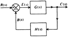
Figure 2.10 General block diagram of a single-loop feedback system.
Solution of these three equations results in the following transfer function relating R(s) and C(s):
For cases where |G(s)H(s)| ≫ 1, the closed-loop transfer function can be approximated by
This implies that the closed-loop transfer function is independent of the direct transmission transfer function G(s), and only depends on the feedback transfer function H(s). Use is made of this characteristic in feedback amplifier design in order that the overall amplifier gain may be insensitive to circuit parameter variations. Note also that the approximate transfer function is the inverse of the feedback transfer function. This property is used for producing behavior which may be difficult to achieve directly.
The characteristic equation for the system can be obtained by setting the denominator of the system transfer function equal to zero:
This equation is known as the characteristic equation and it determines system stability. It will receive much attention in later chapters.
Another useful relationship is the transfer function E(s)/R(s) when H(s) = 1. Then E(s) represents the error, R(s) − C(s). One finds
When |G(s)| ≫ 1, this can be approximated by
Thus the error is small when the magnitude of the open-loop transfer function is large.
Practical feedback systems usually contain multiple feedback loops and several inputs. All multiple-loop systems can be reduced to the basic form shown in Figure 2.10 by means of step-by-step feedback loop reduction, or by means of signal-flow graphs and Mason’s theorem which are considered in Sections 2.14–2.16 of this chapter. Multiple inputs, which are present in all control systems because unwanted inputs (such as noise and drift) are present, can occur anywhere in the feedback system. Successive block-diagram reduction techniques permit the designer to determine their effect on overall performance. Table 2.5 illustrates several transformations that can be used to simplify the reduction of a multiple feedback system. Note that the criterion in transformations 1–4 is to maintain the loop gains constant. The technique of multiple feedback loop reduction can best be understood by means of an example.
Figure 2.11 illustrates a multiple-loop feedback system containing three feedback loops. The original feedback system is illustrated in Figure 2.11a. Figure 2.b–e shows successive steps in reducing this system using the transformations illustrated in Table 2.5. Figure 2.11f shows the resulting closed-loop transfer function of the system.
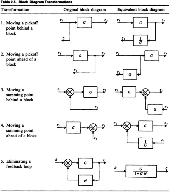

Figure 2.11 Reducing a multiple-loop system containing complex paths. (a) The original system. (b) Rearrangement of the summing points of the intermediate and minor loops. (c) Reduction of the equivalent intermediate loop. (d) Reduction of the equivalent minor loop. (e) The equivalent feedback system. (f) The system transfer function.
Block-diagram reduction techniques get very tedious and time-consuming as the number of feedback paths increases, as is illustrated in Figure 2.11. In order to solve complex problems, it is much simpler to make use of Mason’s theorems and properties of signal-flow graphs, which permit a solution almost by inspection.