
8.8. COMBINED COMPENSATOR DESIGN INCLUDING A CONTROLLER AND AN ESTIMATOR FOR A REGULATOR SYSTEM
This section considers the combined compensator design of a controller and estimator for a regulator in which the reference input equals zero, and for the case where the reference input is finite. The block diagram of this regulator is shown in Figure 8.19, which combines the concepts illustrated in Figure 8.3 for the controller and Figure 8.18 for the estimator. We wish to determine in this system the effect of using the estimated state vector ![]() (t), instead of x(t) on the system dynamics [8].
(t), instead of x(t) on the system dynamics [8].
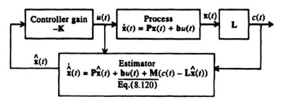
Figure 8.19 Regulator system (where the reference input r = 0) containing combined controller and estimator.
Let us consider the effect of driving the controller with ![]() (t) instead of x(t). From the process dynamics shown in Figure 8.3,
(t) instead of x(t). From the process dynamics shown in Figure 8.3,
From Figure 8.19, we also know that
Therefore, substituting Eq (8.143) into Eq (8.142), we obtain
In terms of the state estimation error ![]() (t) defined in Eq (8.122), Eq (8.144) becomes
(t) defined in Eq (8.122), Eq (8.144) becomes
Combining Eqs. (8.145) and (8.129), we obtain an overall equation for the state vector x and its error ![]() as follows:
as follows:
The characteristic equation of this closed-loop combined controller and estimator system can be obtained in a manner similar to that obtained for the estimator alone [see Eq (8.131)]:
We can write this equation as
The first determinant specifies the characteristic equation of the controller, and the second determinant specified the characteristic equation of the estimator [which is identical to Eq. (8.131)]. As we did for the case of the estimator alone in Section 8.7, Eq. (8.132), we can now define the combined desirable location of estimator roots
(s + α1)(s + α2) ... (s + αn)
and controller roots
(s + β1)(s + β2) ... (s + βn)
and specify the combined estimator and controller’s characteristic equation as
We can now simultaneously determine the controller gain K and estimator coefficients M by setting Eqs. (8.148) and (8.149) equal to each other:
Therefore, we can observe from Eq. (8.150) that the roots of the combined controller and estimator is the sum of the controller and estimator roots found independently [8]. The primary concept to recognize in the combined compensator design for the controller and estimator is to make the estimator respond much faster than the controller, as we do not want the system’s transient response limited by that of the estimator (which we can control by proper design).
It is useful to compare the modern pole placement method using the state-variable feedback method with the conventional transfer-function method for the design of the compensator as we have done in Section 8.2, when we found the open-loop transfer function KG(s)H(s) in terms of h, Φh(s) and b in Eq. (8.25). We wish to find the transfer function of the combined controller and estimator, U(s)/C(s). Let us reconsider the estimator equation, Eq. (8.120), and incorporate it in the control-law equation, Eq. (8.143), because the controller is part of the compensator:
Simplifying, we obtain
Let us compare Eq. (8.152) with the state equation of the process:
whose characteristic equation we know is given by
using the same reasoning we used in obtaining Eqs. (6.22), (8.19), and (8.131). By comparing Eqs. (8.152) and (8.153), we obtain the characteristic equation of the compensator as follows:
The resulting compensator may not result in a stable system because the roots of Eq.(8.155) have not been specified in advance. This is similar to our results in Section 8.3, where we found that design using linear-state-variable feeback did not ensure a stable system.
Before finding the transfer function representing the compensator, U(s)/C(s), we first find the transfer function of the process from Eq. (8.153):
Simplifying,
Solving for X(s), we obtain
Since
c(t) = Lx(t)
and its Laplace transform is
we can combine Eqs. (8.158) and (8.159) to relate the output C(s) and input U(s) of the process.
In order to find the transfer function of the process C(s)/U(s), we assume that the initial condition, x(0), equals zero. Therefore,
By analogy, we compare Eqs. (8.153) [and its resulting transfer function given by Eq.(8.161)] with Eq. (8.153), and conclude that the transfer function of the compensator defined by Eq. (8.152) is given by
When we determine the transfer function U(s)/C(s) using this procedure, we will find that the resulting transfer function will result in a phase-lead network, a phase-lag network, or a phase-lag-lead network.
To illustrate this approach for obtaining the transfer function of the compensator, consider a process whose transfer function is given by
Therefore,
![]() (t) = u(t).
(t) = u(t).
Defining the state variables of this second-order system as
x1(t) = c(t),
x2(t) = ![]() (t),
(t),
we obtain the state equation to be
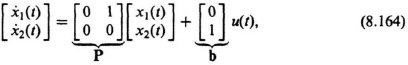
and the output equation is

Let us assume that the design specification for the controller is
ωn = ![]()
ζ = 0.58.
Therefore, the complex-conjugate roots of the controller are located at −1 ± j1.414 and αc(s) for the controller is given by
We can determine the controller gain K by equating like powers of s from Eq. (8.166) and that part of Eq. (8.148) concerned with the controller:
Substituting for P and b from Eq. (8.164) into Eq. (8.167), we obtain the following:
This simplifies to
from which we obtain the characteristic equation of the controller:
Comparing like coefficients in Eqs. (8.166) and (8.170), we find the controller gains to be K1 = 3 and K2 = 2:
As discussed previously, we desire the estimator to have a much faster response than the controller. Therefore, let us assume the design specification of the estimator to be
ωn = 17,
ζ = 0.5
Therefore, the complex-conjugate roots of the estimator are located at −8.5 ± j14.7, and αe(s) for the estimator is given by
The resulting estimator feedback gain matrix is found from Eq. (8.131) [for the estimator portion of Eq. (8.148)] as follows:
Substituting the matrix values into Eq. (8.173), we obtain
which reduces to:
![]()
The resulting characteristic equation in terms of m1 and m2 is given by
Setting like coefficients in Eqs. (8.172) and (8.175) equal to each other, we obtain m1 = 17 and m2 = 288.3:

The resulting compensator transfer function is obtained by substituting parameters obtained from Eqs. (8.164), (8.165), (8.171), and (8.176) into Eq. (8.162) as follows:

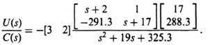
Upon further simplification, we obtain the following:

The resulting transfer function of the compensator is given by the following equation:
Analysis of Eq. (8.179) shows that the compensator has the form of a phase-lead network with a zero at −1.38 and with two complex-conjugate poles as opposed to a simple pole as defined by the conventional phase-lead network of Eq. (7.6).
We can analyze the resulting system using the conventional root-locus and Bode-diagram methods. To obtain the open-loop transfer function for analyses, we combine Eqs. (8.163) and (8.179):
Replacing the specific gain of −627.6 with the variable gain K, the root locus can be evaluated from
which is shown in Figure 8.20. Observe that the root locus goes through the roots chosen in Eqs. (8.166) and (8.172) when K = 627.6. These roots are shown in Figure 8.20 by solid dots. This figure was obtained using MATLAB, and is contained in the M-file that is part of my MCSTD Toolbox which can be retrieved free from The MathWorks, Inc. anonymous FTP server at ftp://ftp.mathworks.comjpubfbooks/shinners.
To draw the Bode diagram, we consider the modified form of Eq. (8.180):
The resulting Bode diagram is drawn from the following simplification to Eq. (8.182):

Figure 8.20 Root locus for compensated system of Figure 8.19 where G(s)Gcomp(s) = (K(s + 1.38))/(s2(s + 9.5 + j15.3)(s + 9.5 − j15.3)).
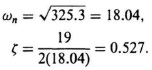
The quadratic poles in the denominator have an undamped natural frequency ωn and a damping ratio ζ given by
The resulting Bode diagram is shown in Figure 8.21. This figure was also obtained using MATLAB and is contained in the M-file that is part of my MCSTD Toolbox.
We conclude that the uncompensated transfer function
G(s) = 1/s2
has its phase margin increased from 0 to 51.07 degrees at its gain crossover frequency of 2.28 rad/sec., and its gain margin is increased from minus infinity to 19.13 dB (phase crossover frequency occurs at ω = 17.32 rad/se) when we use the compensator of Eq. (8.179). Notice that the crossover frequency of 2.28 rad/sec is approximately consistent with the controller’s closed-loop roots of ωn = ![]() = 1.732 rad/sec and ζ = 0.85. This is a reasonable result, as the slower roots of the controller are more dominant than the faster estimator roots, on the system response.
= 1.732 rad/sec and ζ = 0.85. This is a reasonable result, as the slower roots of the controller are more dominant than the faster estimator roots, on the system response.
A complete case study for the design of a combined controller and estimator for a regulator, using the techniques presented in Section 8.7 and 8.8, is presented in Chapter 12.

Figure 8.21 Bode diagram for compensated system of Figure 8.19 where G(s)Gcomp(s) = (((2.66(0.725s + 1))/s2)(325.3/(s2 + 19s + 325.3)).