CHAPTER 4
Working with Excel Ranges and Tables
Most of the work you do in Excel involves cells and ranges. Understanding how best to manipulate cells and ranges will save you time and effort. This chapter discusses a variety of techniques that are essential for Excel users.
Understanding Cells and Ranges
A cell is a single element in a worksheet that can hold a value, some text, or a formula. A cell is identified by its address, which consists of its column letter and row number. For example, cell D9 is the cell in the fourth column and the ninth row.
A group of one or more cells is called a range. You designate a range address by specifying its upper-left cell address and its lower-right cell address, separated by a colon.
Here are some examples of range addresses:
| C24 | A range that consists of a single cell. |
| A1:B1 | Two cells that occupy one row and two columns. |
| A1:A100 | 100 cells in column A. |
| A1:D4 | 16 cells (four rows by four columns). |
| C1:C1048576 | An entire column of cells; this range also can be expressed as C:C. |
| A6:XFD6 | An entire row of cells; this range also can be expressed as 6:6. |
| A1:XFD1048576 | All cells in a worksheet. This range also can be expressed as either A:XFD or 1:1048576. |
Selecting ranges
To perform an operation on a range of cells in a worksheet, you must first select the range. For example, if you want to make the text bold for a range of cells, you must select the range and then choose Home ➪ Font ➪ Bold (or press Ctrl+B).
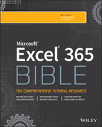
When you select a range, the cells appear highlighted. The exception is the active cell, which remains its normal color. Figure 4.1 shows an example of a selected range (A4:D8) in a worksheet. Cell A4, the active cell, is in the selected range but not highlighted.
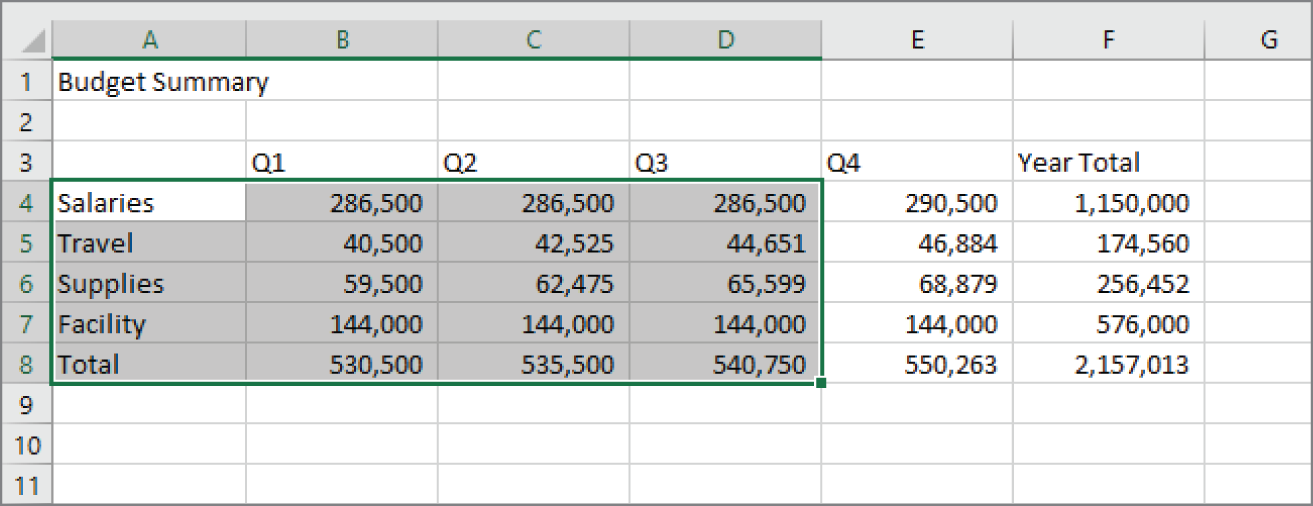
FIGURE 4.1 When you select a range, it appears highlighted, but the active cell within the range is not highlighted.
You can select a range in several ways:
- Left-click and drag over the range. If you drag to the end of the window, the worksheet will scroll.
- Press the Shift key while you use the navigation keys or mouse to select a range.
- Press F8 to enter Extend Selection mode (Extend Selection appears in the status bar). In this mode, click the lower-right cell of the range or use the navigation keys to extend the range. Press F8 again to exit Extend Selection mode.
- Type the cell or range address into the Name box (located to the left of the Formula bar) and press Enter. Excel selects the cell or range that you specified.
- Choose Home ➪ Editing ➪ Find & Select ➪ Go To (or press F5 or Ctrl+G) and enter a range's address manually in the Go To dialog box. When you click OK, Excel selects the cells in the range that you specified.
Selecting complete rows and columns
Often, you'll need to select an entire row or column. For example, you may want to apply the same numeric format or the same alignment options to an entire row or column. You can select entire rows and columns in several ways, including the following:
- Click the row or column header to select a single row or column or click and drag for multiple rows or columns.
- To select multiple (nonadjacent) rows or columns, click the first row or column header and then hold down the Ctrl key while you click the additional row or column header that you want.
- Press Ctrl+spacebar to select the column(s) of the currently selected cells. Press Shift+spacebar to select the row(s) of the currently selected cells.
Selecting noncontiguous ranges
Most of the time, the ranges that you select are contiguous—a single rectangle of cells. Excel also enables you to work with noncontiguous ranges, which consist of two or more ranges (or single cells) that aren't necessarily adjacent to each other. Selecting noncontiguous ranges is also known as a multiple selection. If you want to apply the same formatting to cells in different areas of your worksheet, one approach is to make a multiple selection. When the appropriate cells or ranges are selected, the formatting that you select is applied to all of them. Figure 4.2 shows a noncontiguous range selected in a worksheet. Two ranges are selected: B4:C8 and F15:F17.
You can select a noncontiguous range in the same ways that you select a contiguous range with a few minor differences. Instead of simply clicking and dragging for contiguous ranges, after you select the first range, hold down the Ctrl key while you click and drag to select additional ranges. If you're selecting a range using the arrow keys, select the first range, then press Shift+F8 to enter Add or Remove Selection mode (that term will appear in the status bar). Press Shift+F8 again to exit Add or Remove Selection mode. Anywhere you type the range manually, such as in the Name box or the Go To dialog box, simply separate the noncontiguous ranges with a comma. For example, typing A1:A10,C5:C6 will select those two noncontiguous ranges.
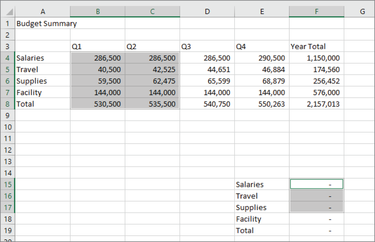
FIGURE 4.2 Excel enables you to select noncontiguous ranges.
Selecting multi-sheet ranges
In addition to two-dimensional ranges on a single worksheet, ranges can extend across multiple worksheets to be three-dimensional ranges.
Suppose you have a workbook set up to track budgets. One approach is to use a separate worksheet for each department, making it easy to organize the data. You can click a sheet tab to view the information for a particular department.
Figure 4.3 shows a simplified example. The workbook has four sheets: Totals, Operations, Marketing, and Manufacturing. The sheets are laid out identically. The only difference is the values. The Totals sheet contains formulas that compute the sum of the corresponding items in the three departmental worksheets.
FIGURE 4.3 The worksheets in this workbook are laid out identically.
Assume that you want to apply formatting to the sheets—for example, to make the column headings bold with background shading. One (albeit not-so-efficient) approach is to format the cells in each worksheet separately. A better technique is to select a multi-sheet range and format the cells in all the sheets simultaneously. The following is a step-by-step example of multi-sheet formatting using the workbook shown in Figure 4.3:
- Activate the Totals worksheet by clicking its tab.
- Select the range B3:F3.
- Press Shift and click the Manufacturing sheet tab. This step selects all worksheets between the active worksheet (Totals) and the sheet tab that you click—in essence, a three-dimensional range of cells (see Figure 4.4). When multiple sheets are selected, the workbook window's title bar displays
Groupto remind you that you've selected a group of sheets and that you're in Group mode.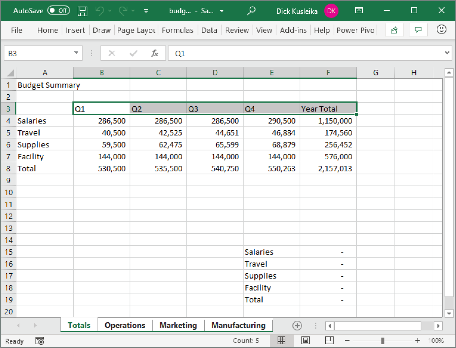
FIGURE 4.4 In Group mode, you can work with a three-dimensional range of cells that extend across multiple worksheets.
- Choose Home ➪ Font ➪ Bold and then choose Home ➪ Font ➪ Fill Color to apply a colored background. Excel applies the formatting to the selected range across the selected sheets.
- Click one of the other sheet tabs. This step selects the sheet and cancels Group mode;
Groupis no longer displayed in the title bar.
When a workbook is in Group mode, any changes that you make to cells in one worksheet also apply to the corresponding cells in all the other grouped worksheets. You can use this to your advantage when you want to set up a group of identical worksheets because any labels, data, formatting, or formulas you enter are automatically added to the same cells in all the grouped worksheets.
In general, selecting a multi-sheet range is a simple two-step process: select the range in one sheet and then select the worksheets to include in the range. To select a group of contiguous worksheets, select the first worksheet in the group and then press Shift and click the sheet tab of the last worksheet that you want to include in the selection. To select individual worksheets, select one of the worksheets in the group and then press Ctrl and click the sheet tab of each additional worksheet that you want to select. If all the worksheets in a workbook aren't laid out the same, you can skip the sheets that you don't want to format. When you make the selection, the sheet tabs of the selected sheets display in bold with underlined text, and Excel displays Group in the title bar.
Selecting special types of cells
As you use Excel, you may need to locate specific types of cells in your worksheets. For example, wouldn't it be handy to be able to locate every cell that contains a formula—or perhaps all the formula cells that depend on the active cell? Excel provides an easy way to locate these and many other special types of cells: select a range and choose Home ➪ Editing ➪ Find & Select ➪ Go To Special to display the Go To Special dialog box, as shown in Figure 4.5.
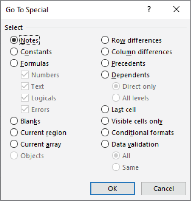
FIGURE 4.5 Use the Go To Special dialog box to select specific types of cells.
After you make your choice in the dialog box, Excel selects the qualifying subset of cells in the current selection. Often, this subset of cells is a multiple selection. If no cells qualify, Excel lets you know with the message No cells were found.
Table 4.1 offers a description of the options available in the Go To Special dialog box.
TABLE 4.1 Go To Special Options
| Option | What it does |
|---|---|
| Notes | Selects the cells that contain a note. |
| Constants | Selects all nonempty cells that don't contain formulas. Use the check boxes under the Formulas option to choose which types of nonformula cells to include. |
| Formulas | Selects cells that contain formulas. Qualify this by selecting the type of result: numbers, text, logical values (TRUE or FALSE), or errors. |
| Blanks | Selects all empty cells. If a single cell is selected when the dialog box is displayed, this option selects the empty cells in the used area of the worksheet. |
| Current Region | Selects a rectangular range of cells around the active cell. This range is determined by surrounding blank rows and columns. You can also press Ctrl+Shift+*. |
| Current Array | Selects the entire array. (See Chapter 10, “Understanding and Using Array Formulas,” for more on arrays.) |
| Objects | Selects all embedded objects on the worksheet, including charts and graphics. |
| Row Differences | Analyzes the selection and selects cells that are different from other cells in each row. |
| Column Differences | Analyzes the selection and selects the cells that are different from other cells in each column. |
| Precedents | Selects cells that are referred to in the formulas in the active cell or selection (limited to the active sheet). You can select either direct precedents or precedents at all levels. (See Chapter 17, “Making Your Formulas Error-Free,” for more information.) |
| Dependents | Selects cells with formulas that refer to the active cell or selection (limited to the active sheet). You can select either direct dependents or dependents at all levels. (See Chapter 17 for more information.) |
| Last Cell | Selects the bottom-right cell in the worksheet that contains data or formatting. For this option, the entire worksheet is examined, even if a range is selected when Excel displays the dialog box. |
| Visible Cells Only | Selects only visible cells in the selection. This option is useful when dealing with a filtered list or a table. |
| Conditional Formats | Selects cells that have a conditional format applied (by choosing Home ➪ Styles ➪ Conditional Formatting). The All option selects all such cells. The Same option selects only the cells that have the same conditional formatting as the active cell. |
| Data Validation | Selects cells that are set up for data entry validation (by choosing Data ➪ Data Tools ➪ Data Validation). The All option selects all such cells. The Same option selects only the cells that have the same validation rules as the active cell. |
Selecting cells by searching
Another way to select cells is to choose Home ➪ Editing ➪ Find & Select ➪ Find (or press Ctrl+F), which allows you to select cells by their contents. The Find and Replace dialog box is shown in Figure 4.6. This figure illustrates additional options that are available when you click the Options button.
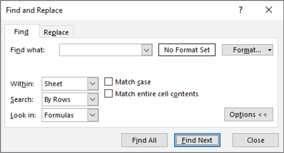
FIGURE 4.6 The Find and Replace dialog box, with its options displayed
Enter the text you're looking for; then click Find All. The dialog box expands to display all the cells that match your search criteria. For example, Figure 4.7 shows the dialog box after Excel has located all cells that contain the text travel. You can click an item in the list, and the screen will scroll so that you can view the cell in context. To select all the cells in the list, first select any single item in the list. Then press Ctrl+A to select them all. You are limited to only selecting cells on the active sheet using this method.
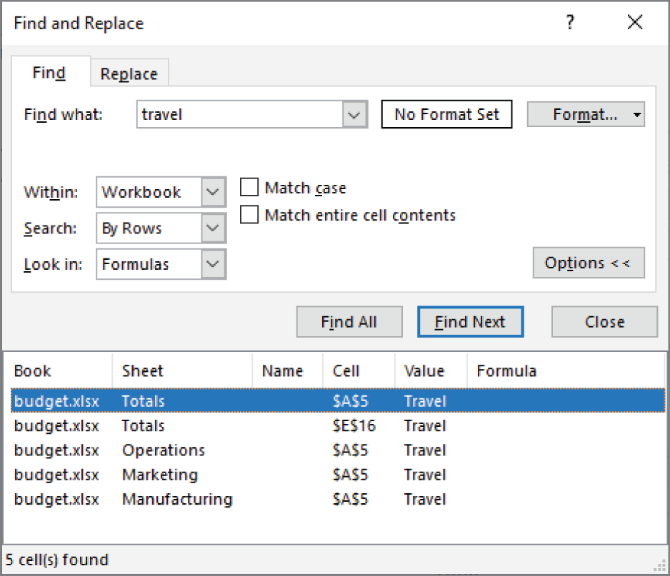
FIGURE 4.7 The Find and Replace dialog box, with its results listed
The Find and Replace dialog box supports two wildcard characters:
?
| Matches any single character |
*
| Matches any number of characters |
Wildcard characters also work with values when the Match Entire Cell Contents option is selected. For example, searching for 3* locates all cells that contain a value that begins with 3. Searching for 1?9 locates all three-digit entries that begin with 1 and end with 9. Searching for *00 locates values that end with two zeros.
If your searches don't seem to be working correctly, double-check these three options:
- Match Case If this check box is selected, the case of the text must match exactly. For example, searching for
smithdoes not locateSmith. - Match Entire Cell Contents If this check box is selected, a match occurs if the cell contains only the search string (and nothing else). For example, searching for
Exceldoesn't locate a cell that containsMicrosoft Excel. When using wildcard characters, an exact match is not required. - Look In This drop-down list has four options: Values, Formulas, Notes, and Comments. The Formulas option looks only at the text that makes up the formula or the contents of the cell if there is no formula. The Values option looks at the cell value and the results, not the text, of the formula. If, for example, Formulas is selected, searching for
900doesn't find a cell that contains the formula=899+1but will find a cell with a value of900. The Values option will find both of those cells.
Copying or Moving Ranges
As you create a worksheet, you may find it necessary to copy or move information from one location to another. Excel makes copying or moving ranges of cells easy. Here are some common things that you might do:
- Copy a cell to another location.
- Copy a cell to a range of cells. The source cell is copied to every cell in the destination range.
- Copy a range to another range.
- Move a cell or range of cells to another location.
The primary difference between copying and moving a range is the effect of the operation on the source range. When you copy a range, the source range is unaffected. When you move a range, the contents are removed from the source range.
Copying or moving consists of two steps (although shortcut methods are available):
- Select the cell or range to copy (the source range) and copy it to the Clipboard. To move the range instead of copying it, cut the range instead of copying it.
- Select the cell or range that will hold the copy (the destination range) and paste the Clipboard contents.
Because copying (or moving) is used so often, Excel provides many different methods. We discuss each method in the following sections. Copying and moving are similar operations, so we point out only important differences between the two.
Copying by using Ribbon commands
Choosing Home ➪ Clipboard ➪ Copy transfers a copy of the selected cell or range to the Windows Clipboard and the Office Clipboard. After performing the copy part of this operation, select the destination cell and choose Home ➪ Clipboard ➪ Paste.
Instead of choosing Home ➪ Clipboard ➪ Paste, you can just activate the destination cell and press Enter. If you use this technique, Excel removes the copied information from the Clipboard so that it can't be pasted again.
If you're copying a range, you don't need to select an entire same-sized range before you click the Paste button. You only need to activate the upper-left cell in the destination range.
Copying by using shortcut menu commands
If you prefer, you can use the following shortcut menu commands for copying and pasting:
- Right-click the range and choose Copy (or Cut) from the shortcut menu to copy the selected cells to the Clipboard.
- Right-click and choose Paste from the shortcut menu that appears to paste the Clipboard contents to the selected cell or range.
For more control over how the pasted information appears, right-click the destination cell and use one of the Paste icons in the shortcut menu (see Figure 4.8).
Instead of using Paste, you can just activate the destination cell and press Enter. If you use this technique, Excel removes the copied information from the Clipboard so that it can't be pasted again.
Copying by using shortcut keys
The copy and paste operations also have shortcut keys associated with them:
- Ctrl+C copies the selected cells to both the Windows Clipboard and the Office Clipboard.
- Ctrl+X cuts the selected cells to both the Windows Clipboard and the Office Clipboard.
- Ctrl+V pastes the Windows Clipboard contents to the selected cell or range.
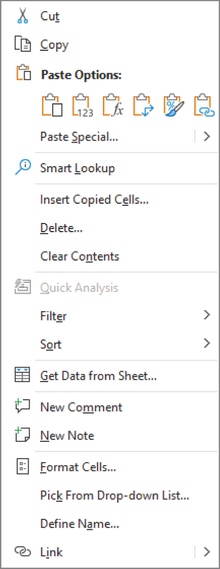
FIGURE 4.8 The Paste icons on the shortcut menu provide more control over how the pasted information appears.
Copying or moving by using drag-and-drop
Excel also enables you to copy or move a cell or range by dragging. Unlike other methods of copying and moving, dragging and dropping does not place any information on either the Windows Clipboard or the Office Clipboard.
To copy using drag-and-drop, select the cell or range that you want to copy, press Ctrl, and move the mouse to one of the selection's borders. (The mouse pointer is augmented with a small plus sign.) Then drag the selection to its new location while you continue to hold down the Ctrl key. The original selection remains behind, and Excel makes a new copy when you release the mouse button.
To move a range using drag-and-drop, don't press Ctrl while dragging the border.
Copying to adjacent cells
Often, you need to copy a cell to an adjacent cell or range. This type of copying is quite common when you're working with formulas. For example, if you're working on a budget, you might create a formula to add the values in column B. You can use the same formula to add the values in the other columns. Rather than re-enter the formula, you can copy it to the adjacent cells.
Excel provides additional options for copying to adjacent cells. To use these commands, activate the cell that you're copying and extend the cell selection to include the cells to which you're copying. Then issue the appropriate command from the following list for one-step copying:
- Home ➪ Editing ➪ Fill ➪ Down (or Ctrl+D) copies the cell to the selected range below.
- Home ➪ Editing ➪ Fill ➪ Right (or Ctrl+R) copies the cell to the selected range to the right.
- Home ➪ Editing ➪ Fill ➪ Up copies the cell to the selected range above.
- Home ➪ Editing ➪ Fill ➪ Left copies the cell to the selected range to the left.
None of these commands places information on either the Windows Clipboard or the Office Clipboard.
Copying a range to other sheets
You can use the copy procedures described previously to copy a cell or range to another worksheet, even if the worksheet is in a different workbook. You must, of course, activate the other worksheet before you select the location to which you want to copy.
Excel offers a quicker way to copy a cell or range and paste it to other worksheets in the same workbook:
- Select the range to copy.
- Press Ctrl and click the sheet tabs for the worksheets to which you want to copy the information. Excel displays
Groupin the workbook's title bar. - Choose Home ➪ Editing ➪ Fill ➪ Across Worksheets. A dialog box appears to ask you what you want to copy (All, Contents, or Formats).
- Make your choice and then click OK. Excel copies the selected range to the selected worksheets; the new copy occupies the same cells in the selected worksheets as the original occupies in the initial worksheet.
Using the Office Clipboard to paste
Whenever you cut or copy information in an Office program such as Excel, you can place the data on both the Windows Clipboard and the Office Clipboard. When you copy information to the Office Clipboard, you append the information to the Office Clipboard instead of replacing what is already there. With multiple items stored on the Office Clipboard, you can then paste the items either individually or as a group.
To use the Office Clipboard, you first need to open it. Use the dialog box launcher on the bottom right of the Home ➪ Clipboard group to toggle the Clipboard task pane on and off.
After you open the Clipboard task pane, select the first cell or range that you want to copy to the Office Clipboard and copy it by using any of the preceding techniques. Repeat this process, selecting the next cell or range that you want to copy. As soon as you copy the information, the Office Clipboard task pane shows you the number of items that you've copied and a brief description (it will hold up to 24 items). Figure 4.9 shows the Office Clipboard with five copied items.
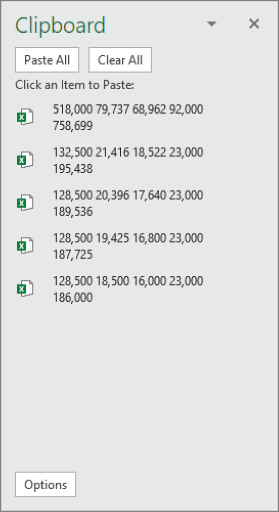
FIGURE 4.9 Use the Clipboard task pane to copy and paste multiple items.
When you're ready to paste information, select the cell into which you want to paste it. To paste an individual item, click it in the Clipboard task pane. To paste all the items that you've copied, click the Paste All button (which is at the top of the Clipboard task pane). The items are pasted, one after the other. The Paste All button is probably more useful in Word for situations in which you copy text from various sources and then paste it all at once.
You can clear the contents of the Office Clipboard by clicking the Clear All button.
The following items about the Office Clipboard and how it functions are worth noting:
- Excel pastes the contents of the Windows Clipboard (the last item you copied to the Office Clipboard) when you paste by choosing Home ➪ Clipboard ➪ Paste, by pressing Ctrl+V, or by right-clicking and choosing Paste from the shortcut menu.
- The last item that you cut or copied appears on both the Office Clipboard and the Windows Clipboard.
- Clearing the Office Clipboard also clears the Windows Clipboard.
Pasting in special ways
You may not always want to copy everything from the source range to the destination range. For example, you may want to copy only the formula results rather than the formulas themselves. Or you may want to copy the number formats from one range to another without overwriting any existing data or formulas.
To control what is copied into the destination range, choose Home ➪ Clipboard ➪ Paste and use the drop-down menu shown in Figure 4.10. When you hover your mouse pointer over an icon, you'll see a preview of the pasted information in the destination range. Click the icon to use the selected paste option.
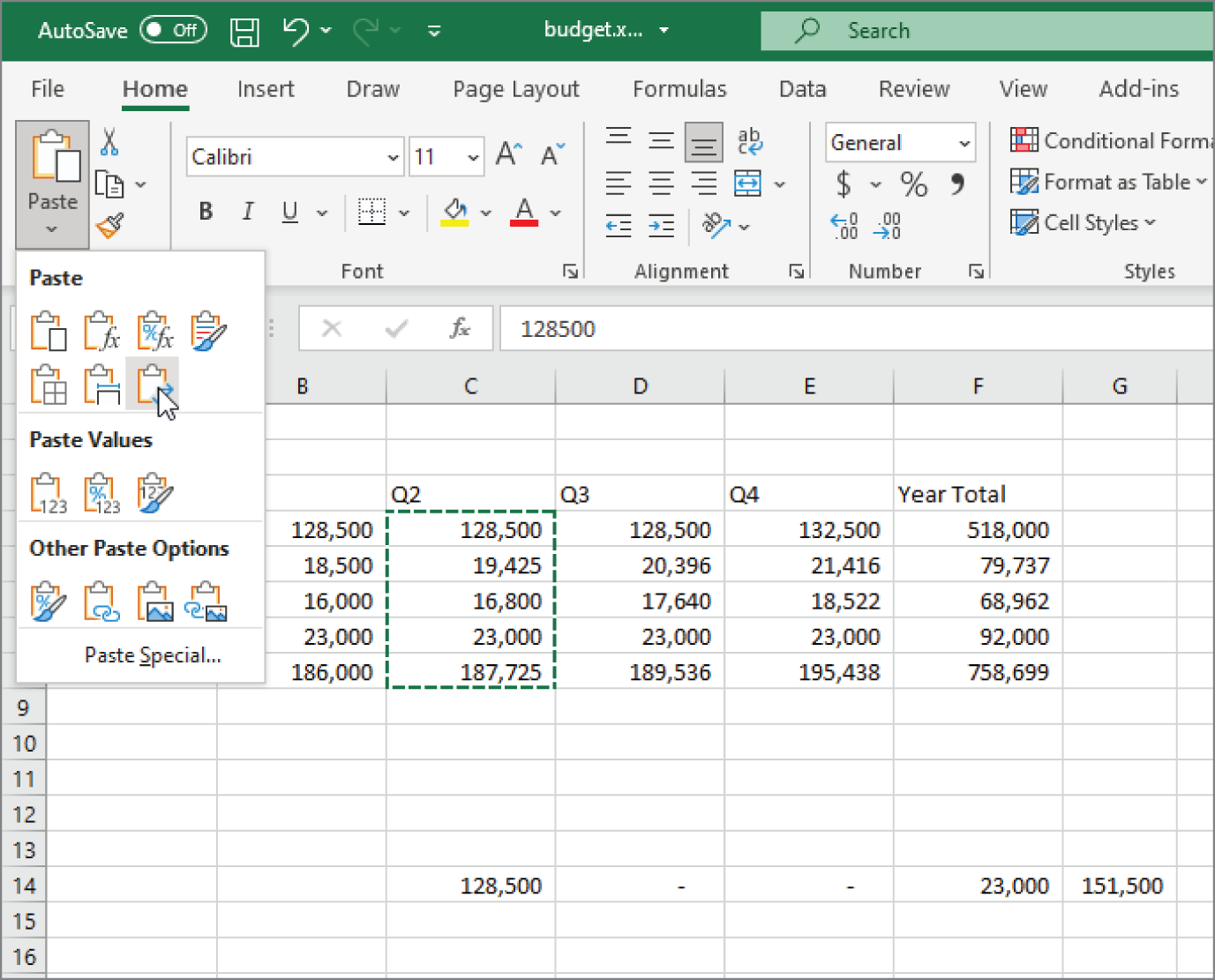
FIGURE 4.10 Excel offers several pasting options, with preview. Here, the information is copied from C4:C8 and is being pasted beginning at cell C14 using the Transpose option.
The paste options are as follows:
- Paste (P) Pastes the cell's contents, formula, formats, and data validation from the Windows Clipboard.
- Formulas (F) Pastes formulas but not formatting.
- Formulas & Number Formatting (O) Pastes formulas and number formatting only.
- Keep Source Formatting (K) Pastes formulas and all formatting.
- No Borders (B) Pastes everything except borders that appear in the source range.
- Keep Source Column Widths (W) Pastes formulas and duplicates the column width(s) of the copied cells.
- Transpose (T) Changes the orientation of the copied range. Rows become columns, and columns become rows. Any formulas in the copied range are adjusted so that they work properly when transposed.
- Merge Conditional Formatting (G) This icon is displayed only when the copied cells contain conditional formatting. When clicked, it merges the copied conditional formatting with any conditional formatting in the destination range.
- Values (V) Pastes the results of formulas. The destination for the copy can be a new range or the original range. In the latter case, Excel replaces the original formulas with their current values.
- Values & Number Formatting (A) Pastes the results of formulas plus the number formatting.
- Values & Source Formatting (E) Pastes the results of formulas plus all formatting.
- Formatting (R) Pastes only the formatting of the source range.
- Paste Link (N) Creates formulas in the destination range that refer to the cells in the copied range.
- Picture (U) Pastes the copied information as a picture.
- Linked Picture (I) Pastes the copied information as a “live” picture that is updated if the source range is changed.
- Paste Special Displays the Paste Special dialog box (described in the next section).
Using the Paste Special dialog box
For yet another pasting method, choose Home ➪ Clipboard ➪ Paste ➪ Paste Special to display the Paste Special dialog box (see Figure 4.11). You can also right-click and choose Paste Special from the shortcut menu to display this dialog box. This dialog box has several options, some of which are identical to the buttons in the Paste drop-down menu. The options that are different are explained in the following list.
- Comments and Notes Copies only the cell comments and cell notes from a cell or range. This option doesn't copy cell contents or formatting.
- Validation Copies the validation criteria so that the same data validation will apply. Data validation is applied by choosing Data ➪ Data Tools ➪ Data Validation.
- All using Source theme Pastes everything but uses the formatting from the document theme of the source. This option is relevant only if you're pasting information from a different workbook and the workbook uses a different document theme than the active workbook.
- Column widths Pastes only column width information.
- All merging conditional formats Merges the copied conditional formatting with any conditional formatting in the destination range. This option is enabled only when you're copying a range that contains conditional formatting.
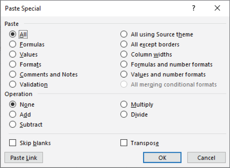
FIGURE 4.11 The Paste Special dialog box
In addition, the Paste Special dialog box enables you to perform other operations, described in the following sections.
Performing mathematical operations without formulas
The option buttons in the Operation section of the Paste Special dialog box let you perform an arithmetic operation on values and formulas in the destination range. For example, you can copy a range to another range and select the Multiply operation. Excel multiplies the corresponding values in the source range and the destination range and replaces the destination range with the new values.
This feature also works with a single copied cell, pasted to a multicell range. Assume that you have a range of values, and you want to increase each value by 5 percent. Enter 105% into any blank cell and copy that cell to the Clipboard. Then select the range of values and bring up the Paste Special dialog box. Select the Multiply option, and each value in the range is multiplied by 105%.
Skipping blanks when pasting
The Skip Blanks option in the Paste Special dialog box prevents Excel from overwriting cell contents in your paste area with blank cells from the copied range. This option is useful if you're copying a range to another area but don't want the blank cells in the copied range to overwrite existing data.
Transposing a range
The Transpose option in the Paste Special dialog box changes the orientation of the copied range. Rows become columns, and columns become rows. Any formulas in the copied range are adjusted so that they work properly when transposed. Note that you can use this check box with the other options in the Paste Special dialog box. Figure 4.12 shows an example of a horizontal range (A3:F8) that was transposed to a different range (A11:F16).
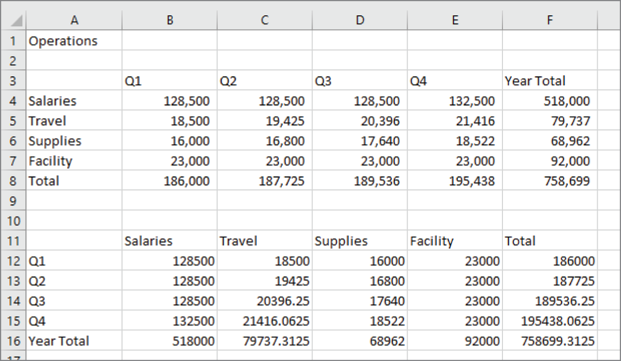
FIGURE 4.12 Transposing a range changes the orientation as the information is pasted into the worksheet.
Using Names to Work with Ranges
Dealing with cryptic cell and range addresses can sometimes be confusing, especially when you work with formulas, which we cover in Chapter 9, “Introducing Formulas and Functions.” Fortunately, Excel allows you to assign descriptive names to cells and ranges. For example, you can give a cell a name such as Interest_Rate, or you can name a range JulySales. Working with these names (rather than cell or range addresses) has several advantages:
- A meaningful range name (such as Total_Income) is much easier to remember than a cell address (such as AC21).
- Entering a name is less error prone than entering a cell or range address, and if you type a name incorrectly in a formula, Excel will display a
#NAME?error. - You can quickly move to areas of your worksheet either by using the Name box, located at the left side of the Formula bar (click the arrow to drop down a list of defined names) or by choosing Home ➪ Editing ➪ Find & Select ➪ Go To (or pressing F5 or Ctrl+G) and specifying the range name.
- Creating formulas is easier. You can paste a cell or range name into a formula by using Formula AutoComplete.
- Names make your formulas more understandable and easier to use. A formula such as
=Income—Taxesis certainly more intuitive than=D20—D40.
Creating range names in your workbooks
Excel provides several methods that you can use to create range names. Before you begin, however, you should be aware of a few rules:
- Names can't contain spaces. You may want to use an underscore character to simulate a space (such as Annual_Total).
- You can use any combination of letters and numbers, but the name must begin with a letter, underscore, or backslash. A name can't begin with a number (such as 3rdQuarter) or look like a cell address (such as QTR3). If these are desirable names, though, you can precede the name with an underscore or a backslash, for example, _3rdQuarter and QTR3.
- Symbols—except for underscores, backslashes, and periods—aren't allowed.
- Names are limited to 255 characters, but it's a good practice to keep names as short as possible yet still meaningful.
Using the Name box
The fastest way to create a name is to use the Name box (to the left of the Formula bar). Select the cell or range to name, click the Name box, and type the name. Press Enter to create the name. (You must press Enter to actually record the name; if you type a name and then click in the worksheet, Excel doesn't create the name.)
If you type an invalid name (such as May21, which happens to be a cell address, MAY21), Excel activates that address and doesn't warn you that the name is not valid. If the name you type includes an invalid character, Excel displays an error message. If a name already exists, you can't use the Name box to change the range to which that name refers. Attempting to do so simply selects the range.
The Name box is a drop-down list and shows all names in the workbook. To choose a named cell or range, click the arrow on the right side of the Name box and choose the name. The name appears in the Name box, and Excel selects the named cell or range in the worksheet.
Using the New Name dialog box
For more control over naming cells and ranges, use the New Name dialog box. Start by selecting the cell or range that you want to name. Then choose Formulas ➪ Defined Names ➪ Define Name. Excel displays the New Name dialog box, shown in Figure 4.13. Note that this is a resizable dialog box. Click and drag a border to change the dimensions.
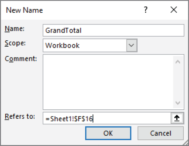
FIGURE 4.13 Create names for cells or ranges by using the New Name dialog box.
Type a name in the Name text field (or use the name that Excel proposes, if any). The selected cell or range address appears in the Refers To text field. Use the Scope drop-down list to indicate the scope for the name. The scope indicates where the name will be valid, and it's either the entire workbook or the worksheet in which the name is defined. If you like, you can add a comment that describes the named range or cell. Click OK to add the name to your workbook and close the dialog box.
Using the Create Names from Selection dialog box
You may have a worksheet that contains text that you want to use for names for adjacent cells or ranges. For example, you may want to use the text in column A to create names for the corresponding values in column B. Excel makes this task easy.
To create names by using adjacent text, start by selecting the name text and the cells that you want to name. (These items can be individual cells or ranges of cells.) The names must be adjacent to the cells that you're naming. (A multiple selection is allowed.) Then choose Formulas ➪ Defined Names ➪ Create from Selection. Excel displays the Create Names from Selection dialog box, shown in Figure 4.14.
The check marks in the Create Names from Selection dialog box are based on Excel's analysis of the selected range. For example, if Excel finds text in the first row of the selection, it proposes that you create names based on the top row. If Excel didn't guess correctly, you can change the check boxes. Click OK, and Excel creates the names. Using the data in Figure 4.14, Excel creates the seven named ranges shown in Figure 4.15.
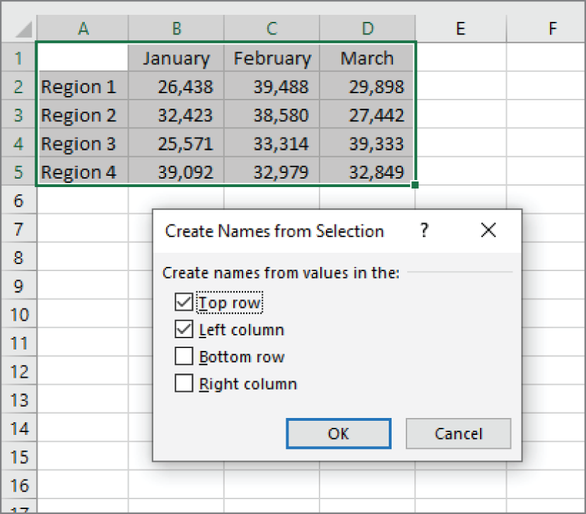
FIGURE 4.14 Use the Create Names from Selection dialog box to name cells using labels that appear in the worksheet.
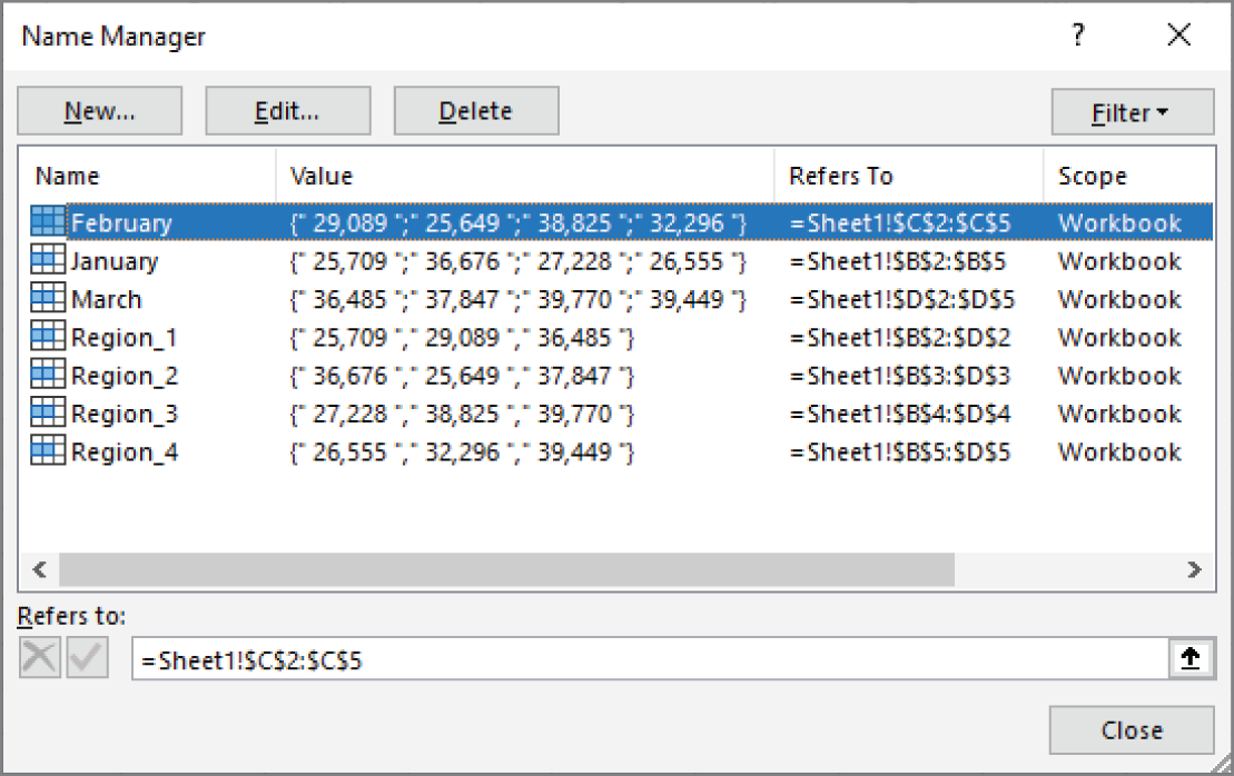
FIGURE 4.15 Use the Name Manager to work with range names.
Managing names
A workbook can have any number of named cells and ranges. If your workbook has many names, you should know about the Name Manager, which is shown in Figure 4.15.
The Name Manager appears when you choose Formulas ➪ Defined Names ➪ Name Manager (or press Ctrl+F3). The Name Manager has the following features:
- Displays information about each name in the workbook You can resize the Name Manager dialog box, widen the columns to show more information, and even rearrange the order of the columns. You can also click a column heading to sort the information by the column.
- Allows you to filter the displayed names Clicking the Filter button lets you show only those names that meet certain criteria. For example, you can view only the worksheet-level names.
- Provides quick access to the New Name dialog box Click the New button to create a new name without closing the Name Manager.
- Lets you edit names To edit a name, select it in the list, and then click the Edit button or double-click the name. You can change the name itself, modify the Refers To range, or edit the comment.
- Lets you quickly delete unneeded names To delete a name, select it in the list and click Delete.
If you delete the rows or columns that contain named cells or ranges, the names contain an invalid reference. For example, if cell A1 on Sheet1 is named Interest and you delete row 1 or column A, the name Interest then refers to =Sheet1!#REF! (an erroneous reference). If you use the name Interest in a formula, the formula displays #REF!.
Adding Comments to Cells
In recent versions of Excel, Microsoft has added a new way to annotate cells. Prior to this change, you could add a comment to a cell; the comment consisted of a simple text box containing whatever text you wished to add. What used to be called a comment is now called a note and is discussed in the next section. The new method of annotation is called a comment. It is a threaded list of comments and is designed to facilitate a conversation among users.
To add a comment to a cell, select the cell and perform any of these commands:
- Choose Review ➪ Comments ➪ New Comment.
- Right-click the cell and choose New Comment from the shortcut menu.
- Press Ctrl+Shift+F2.
Excel attaches a new, blank comment to the cell, as shown in Figure 4.16. To complete the comment, type in the Start a conversation text box and click the Post button. If you don't type anything and click Post, the comment will not be created. When you post, Excel creates the comment including which user posted it and the date and time it was posted. Figure 4.17 shows a completed comment.
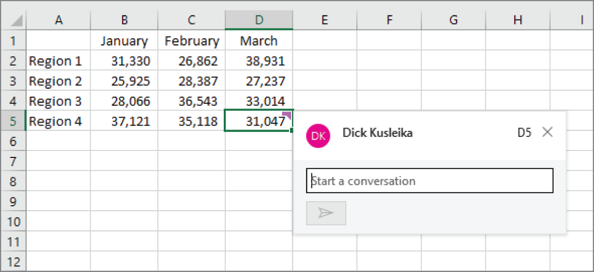
FIGURE 4.16 Creating a comment attaches a new, blank comment to a cell.
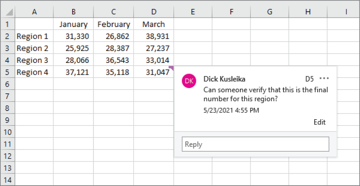
FIGURE 4.17 Typing a comment and clicking the Post button finishes the comment creation process.
Showing comments
Cells with comments have a small mark in the upper-right corner. To view a comment thread for a cell, select the cell that contains it. Hovering your mouse over the cell will display the comment, but it will disappear when you move your mouse away. Clicking on a comment while it's displayed will select the cell. You can also right-click on the cell and choose Reply to Comment to view it.
To see all the comments on the worksheet, chose Review ➪ Comments ➪ Show Comments. This action opens the Comments task pane that lists all the comments on the active worksheet. Figure 4.18 shows two comment threads, one in cell B3 and one in cell D5 that also includes a reply.
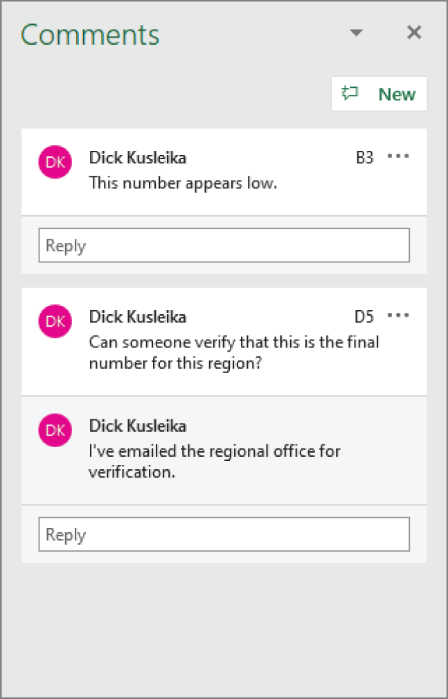
FIGURE 4.18 Showing all comments in the Comments task pane.
The Comments task pane allows you to create new comments and reply to existing ones. The New button will create a new comment if the active cell doesn't already contain a comment or will put the cursor in the reply box for the comment already attached to the active cell.
The Ribbon contains two commands to cycle through all the comments on the worksheet: Choose Review ➪ Comments ➪ Previous Comment or Review ➪ Comments ➪ Next Comment to move through the comments. If the Comments task pane is visible, these actions will select the comments in the task pane. If it's not visible, the comments will appear next to the cells to which they're attached.
Replying to comments
Each comment has a Reply box for entering additional text, threaded underneath the comment you reply to. When you start a reply, the comment box displays Post and Cancel buttons to complete the reply. You can only reply to the last comment in the thread.
Editing comments and replies
The comment box contains an Edit button that allows you to change the text of the comment if you are the user that created it. Editing a comment does not update the date and time stamp on it. Replies also have an Edit button if you are the user who replied. The Edit button is only visible when that comment or reply is active or your mouse is hovering over it.
When you're editing a comment, Save and Cancel buttons are displayed to confirm your edits or revert to the old text.
Deleting comments and replies
The first comment in a thread has an ellipsis in the upper-right corner. This menu contains two entries: Delete Thread and Resolve Thread (discussed in the next section), as shown in Figure 4.19. Clicking Delete Thread deletes the comment and all comments below it. You can also right-click on the cell and choose Delete Comment or choose Review ➪ Comments ➪ Delete to delete the entire thread. If you delete a thread by mistake, choose Undo from the Quick Access Toolbar or press Ctrl+Z.
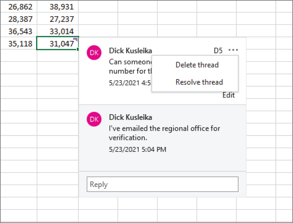
FIGURE 4.19 The first comment in a thread has an ellipsis menu to delete the thread.
Replies to comments have a Delete button instead of the ellipsis menu. When you click Delete on a reply, only that reply is deleted. Any replies below the deleted reply remain in the thread.
Resolving comment threads
The other menu item in the ellipsis menu is Resolve Thread. When you resolve a thread, you prevent any more replies from being posted to it. Resolved threads are grayed out and two new buttons appear at the bottom of the thread: Reopen Thread and Delete Thread. Figure 4.20 shows a comment that has been resolved.
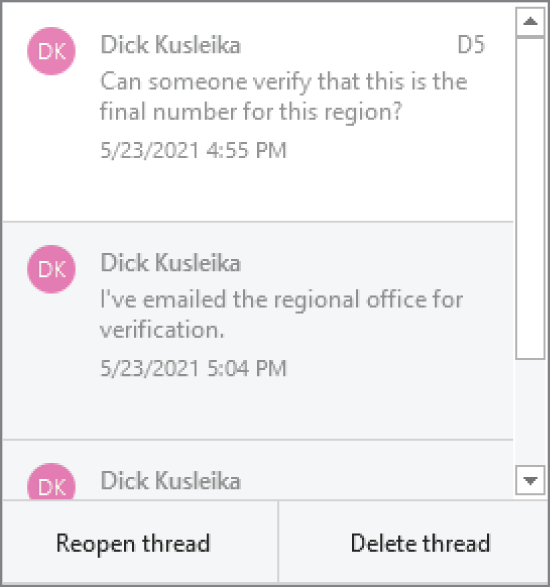
FIGURE 4.20 A resolved comment is grayed out and buttons to reopen or delete are displayed at the bottom.
Reopening a thread changes it back to its state prior to being resolved. That is, it's no longer grayed out and users can reply to it. Anyone with write access to the workbook can resolve or reopen threads, not just the user who created it. Deleting a resolved thread works just like deleting an open thread. The advantage of resolving a thread is to signal to other users that all the issues have been handled but to keep the thread there as an artifact. Resolved threads still show on the Comments task pane and are still displayed if you cycle through all the threads.
Adding Notes to Cells
What used to be called a comment is now called a note. Notes are simple text boxes that are attached to cells. While they are simple, they support resizing and some formatting. Unlike the new comment feature, you can't reply to a note, but you can add additional text to the bottom of it. Notes are useful when you need to describe a particular value or explain how a formula works.
To add a note to a cell, select the cell and use any of these actions:
- Choose Review ➪ Notes ➪ Notes ➪ New Note.
- Right-click the cell and choose New Note from the shortcut menu.
- Press Shift+F2.
Excel inserts a note that points to the active cell. Initially, the note consists of your name, as specified in the General tab of the Excel Options dialog box (choose File ➪ Options to display this dialog box). If you like, you can delete your name from the note. Enter the text for the cell note and then click anywhere in the worksheet to hide the note. You can change the size of the note by clicking and dragging any one of its eight sizing handles. Figure 4.21 shows a cell with a note.
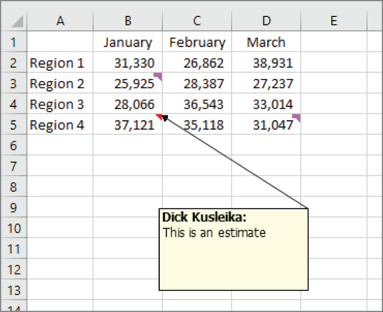
FIGURE 4.21 You can add a note to a cell to help document your worksheets.
Cells that have a note display a small red triangle in the upper-right corner. When you move the mouse pointer over a cell that contains a note, the note becomes visible.
You can force a note to be displayed even when the mouse is not hovering over the cell. Right-click the cell and choose Show/Hide Note. The menu item toggles between always showing the note and returning to just the red triangle and only displaying the note when you hover over it.
Showing notes
If you want all cell notes to be visible (regardless of the location of the mouse), choose Review ➪ Notes ➪ Notes ➪ Show All Notes. This command is a toggle; select it again to hide all cell notes.
To toggle the display of an individual note, select its cell and then choose Review ➪ Notes ➪ Notes ➪ Show/Hide Note. The Notes button in the Notes group on the Ribbon also contains a Next Note and a Previous Note command. Choosing one of these commands displays the next or previous note and hides the current one, if any.
Formatting notes
If you don't like the default look of cell notes, you can make some changes. Right-click the cell and choose Edit Note. Select the text in the note and use the commands of the Font and the Alignment groups on the Home tab to make changes to the note's appearance.
For even more formatting options, choose Home ➪ Cells ➪ Format ➪ Format Comment or right-click on the note's border and choose Format Comment from the shortcut menu. Excel responds by displaying the Format Comment dialog box, which allows you to change many aspects of a comment's appearance, including color, border, and margins.
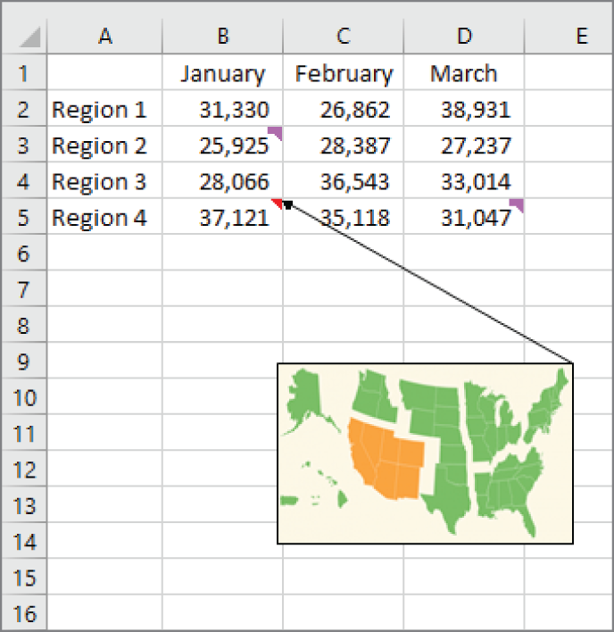
FIGURE 4.22 This note contains an image.
Editing notes
To edit the text in a note, activate the cell, right-click, and then choose Edit Note from the shortcut menu. Or select the cell and press Shift+F2. After you make your changes, click any cell.
Deleting notes
To delete a cell note, activate the cell that contains the note and then choose Review ➪ Comments ➪ Delete. Or right-click and then choose Delete Note from the shortcut menu.
Working with Tables
A table is a specially designated area of a worksheet. When you designate a range as a table, Excel gives it special properties that make certain operations easier and that help prevent errors.
The purpose of a table is to enforce some structure around your data. If you're familiar with a table in a database (like Microsoft Access), then you already understand the concept of structured data. If not, don't worry. It's not difficult.
In a table, each row contains information about a single entity. In a table that holds employee information, each row will contain information about one employee (such as name, department, and hire date). Each column contains the same piece of information for each employee. The same column that holds the hire date for the first employee holds the hire date for all the other employees.
Understanding a table's structure
Figure 4.23 shows a simple table. The various components of a table are described in the following sections.
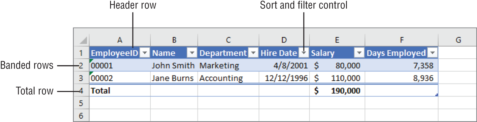
FIGURE 4.23 The areas that make up a table
The header row
The header row is generally colored differently than the other rows. The names in the header identify the columns. If you have a formula that refers to a table, the header row will determine how the column is referred to. For example, the Days Employed column (column F) contains a formula that refers to the Hire Date column (column D). The formula is =NOW()-[@[Hire Date]]. If your table is longer than one screen, the header row will replace the normal column headers in Excel when you scroll down.
The header also contains Filter Buttons. These drop-down buttons work exactly like Excel's normal AutoFilter feature. You can use them to sort and filter the table's data.
The data body
The data body is one or more rows of data. By default, the rows are banded, that is, formatted with alternating colors. When you add new data to the table, the formatting of the existing data is applied to the new data. For example, if a column is formatted as Text, that column in the new row will also be formatted as Text. The same is true for conditional formatting.
It's not just formatting that applies to the new data. If a column contains a formula, that formula is automatically inserted into the new row. Data validation will also be transferred. You can make a robust data entry area knowing that the table structure will apply to new data.
One of the best features of tables is that as the data body expands, anything that refers to the table will expand automatically. If you were to base a PivotTable or a chart on your table, the PivotTable or chart would adjust as you added or deleted rows from the table.
The total row
The total row is not visible by default when you create a table. To show the total row, check the Total Row check box in the Table Style Options group on the Table Design Ribbon. When you show the total row, the text Total is placed in the first column. You can change this to another value or to a formula.
Each cell in the total row has a drop-down arrow with a list of common functions. It's no accident that the list of functions resembles the arguments for the SUBTOTAL function. When you select a function from the list, Excel inserts a SUBTOTAL formula in the cell. The SUBTOTAL function ignores filtered cells, so the total will change if you filter the table.
In addition to the list of functions in the total row, there is a More Functions option at the bottom of the drop-down list. Selecting this option shows the Insert Function dialog box and makes all of Excel's functions available to you. Beyond that, you can simply type whatever formula you want in the total row.
The resizing handle
At the bottom right of the last cell in the table is the resizing handle. You can drag this handle to change the size of the table. Increasing the length of the table adds blank rows, copying down formatting, formulas, and data validation. Increasing the width of the table adds new columns with generic names like Column1, Column2, and so forth. You can change those names to something more meaningful.
Decreasing the size of the table simply changes what data is considered part of the table. It does not delete any data, formatting, formulas, or data validation. If you want to change what's in your table, you're better off deleting the columns and rows as you would any range rather than trying to do it with the resizing handle.
Creating a table
Most of the time, you'll create a table from an existing range of data. However, Excel also allows you to create a table from an empty range so that you can fill in the data later. The following instructions assume that you already have a range of data that's suitable for a table:
- Make sure the range doesn't contain any completely blank rows or columns; otherwise, Excel will not guess the table range correctly.
- Select any cell within the range.
- Choose Insert ➪ Tables ➪ Table (or press Ctrl+T). Excel responds with its Create Table dialog box, shown in Figure 4.24. Excel tries to guess the range, as well as whether the table has a header row. Most of the time, it guesses correctly. If not, make your corrections before you click OK.
The range is converted to a table (using the default table style), and the Table Design tab of the Ribbon appears.
To create a table from an empty range, select the range and choose Insert ➪ Tables ➪ Table. Excel creates the table, adds generic column headers (such as Column1 and Column2), and applies table formatting to the range. Almost always, you'll want to replace the generic column headers with more meaningful text.
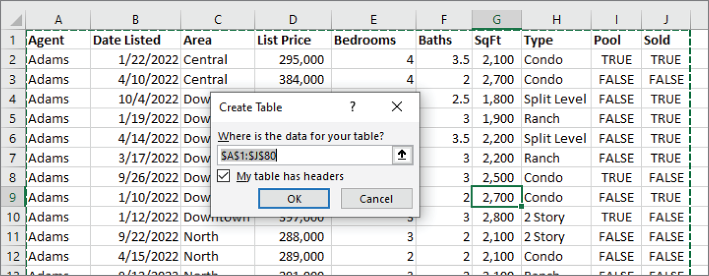
FIGURE 4.24 Use the Create Table dialog box to verify that Excel guessed the table dimensions correctly.
Adding data to a table
If your table doesn't have a total row, the easiest way to enter data is simply to start typing in the row just below the table. When you enter something in a cell, Excel automatically expands the table and applies the formatting, formulas, and data validation to the new row. You can also paste a value in the next row. In fact, you could paste several rows' worth of data and the table will expand to accommodate.
If your table has a total row, you can't use that technique. In that case, you can insert rows into a table just as you would insert a row into any range. To insert a row, select a cell or the entire row and choose Home ➪ Cells ➪ Insert. When the selected range is inside a table, you'll see new entries on the Insert menu that deal with tables specifically. When you use these, the table is changed, but the data outside the table is unaffected.
When the selected cell is inside a table, the shortcut keys Ctrl− (minus sign) and Ctrl+ (plus sign) work on the table only and not on data outside the table. Moreover, as opposed to when you're not in a table, those shortcuts work on the whole table row or column regardless of whether you've selected the whole row or column.
Sorting and filtering table data
Each item in the header row of a table contains a drop-down arrow known as a Filter Button. When clicked, the Filter Button displays sorting and filtering options (see Figure 4.25).
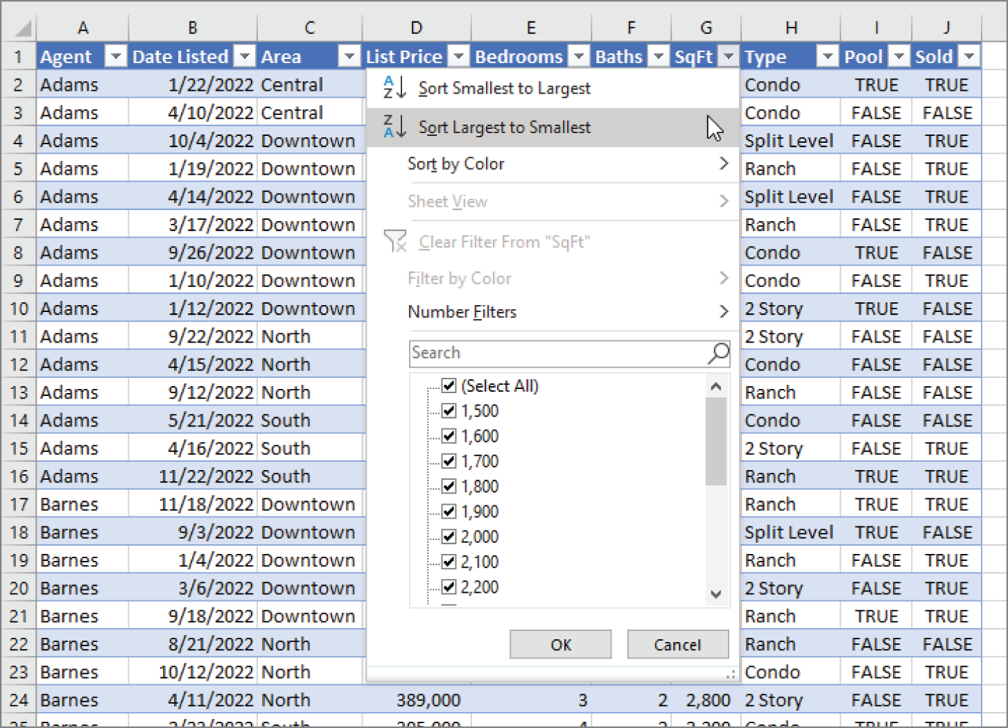
FIGURE 4.25 Each column in a table has sorting and filtering options.
Sorting a table
Sorting a table rearranges the rows based on the contents of a particular column. You may want to sort a table to put names in alphabetical order. Or maybe you want to sort your sales staff by the total sales made.
To sort a table by a particular column, click the Filter Button in the column header and choose one of the sort commands. The exact command varies, depending on the type of data in the column.
You can also select Sort by Color to sort the rows based on the background or text color of the data. This option is relevant only if you've overridden the table style colors with custom formatting.
You can sort on any number of columns. The trick is to sort the least significant column first and then proceed until the most significant column is sorted last. For example, in the real estate table, you may want to sort the list by agent. And within each agent's group, sort the rows by area. Then within each area, sort the rows by list price in descending order. For this type of sort, first sort by the Agent column, then sort by the Area column, and then sort by the List Price column. Figure 4.26 shows the table sorted in this manner.
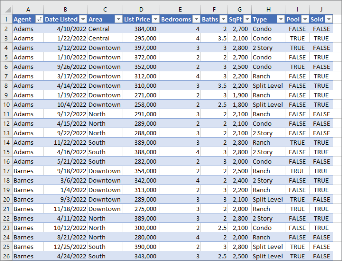
FIGURE 4.26 A table after performing a three-column sort
Another way of performing a multiple-column sort is to use the Sort dialog box (choose Home ➪ Editing ➪ Sort & Filter ➪ Custom Sort). Or right-click any cell in the table and choose Sort ➪ Custom Sort from the shortcut menu.
In the Sort dialog box, use the drop-down lists to specify the sort specifications. In this example, you start with Agent. Then click the Add Level button to insert another set of search controls. In this new set of controls, specify the sort specifications for the Area column. Then add another level and enter the specifications for the List Price column. Figure 4.27 shows the dialog box after entering the specifications for the three-column sort. This technique produces the same sort as described previously.
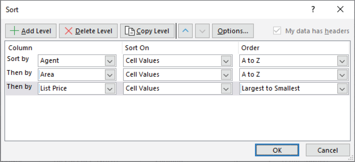
FIGURE 4.27 Using the Sort dialog box to specify a three-column sort
Filtering a table
Filtering a table refers to displaying only the rows that meet certain conditions. (The other rows are hidden.)
Note that entire worksheet rows are hidden. Therefore, if you have other data to the left or right of your table, that information may also be hidden when you filter the table. If you plan to filter your list, don't include any other data to the left or right of your table.
Using the real estate table, assume that you're interested only in the data for the Downtown area. Click the Filter Button in the Area row header and remove the check mark from Select All, which deselects everything. Then place a check mark next to Downtown and click OK. The table, shown in Figure 4.28, is now filtered to display only the listings in the Downtown area. Notice that some of the row numbers are missing. These rows are hidden and contain data that does not meet the specified criteria.
Also notice that the Filter Button in the Area column now shows a different graphic—an icon that indicates the column is filtered.
You can filter by multiple values in a column using multiple check marks. For example, to filter the table to show only Downtown and Central, place a check mark next to both values in the drop-down list in the Area row header.
You can filter a table using any number of columns. For example, you may want to see only the Downtown listings in which the Type is Condo. Just repeat the operation using the Type column. The table then displays only the rows in which the Area is Downtown and the Type is Condo.
For additional filtering options, select Text Filters (or Number Filters, if the column contains values). The options are fairly self-explanatory, and you have a great deal of flexibility in displaying only the rows in which you're interested. For example, you can display rows in which the List Price is greater than or equal to $200,000 and less than $300,000 (see Figure 4.29).
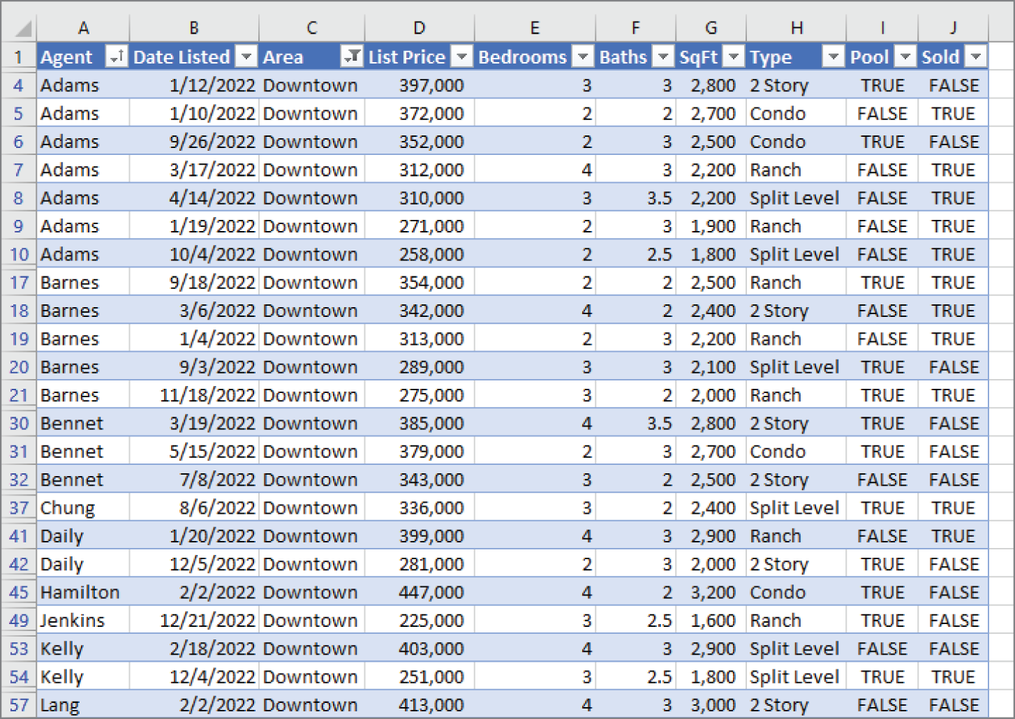
FIGURE 4.28 This table is filtered to show the information for only one area.
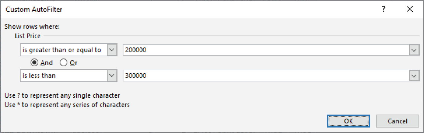
FIGURE 4.29 Specifying a more complex numeric filter
Also, you can right-click a cell and use the Filter command on the shortcut menu. This menu item leads to several additional filtering options that enable you to filter data based on the contents of the selected cell or by formatting.
When you copy data from a filtered table, only the visible data is copied. In other words, rows that are hidden by filtering aren't copied. This filtering makes it easy to copy a subset of a larger table and paste it to another area of your worksheet. Keep in mind, though, that the pasted data is not a table—it's just a normal range. You can, however, convert the copied range to a table.
To remove filtering for a column, click the drop-down in the row header and select Clear Filter. If you've filtered using multiple columns, it may be faster to remove all filters by choosing Data ➪ Sort & Filter ➪ Clear.
Filtering a table with slicers
Another way to filter a table is to use one or more slicers. This method is less flexible but more visually appealing. Slicers are particularly useful when the table will be viewed by novices or those who find the normal filtering techniques too complicated. Slicers are very visual, and it's easy to see exactly what type of filtering is in effect. A disadvantage of slicers is that they take up a lot of room on the screen.
To add one or more slicers, activate any cell in the table and choose Table Design ➪ Tools ➪ Insert Slicer. Excel responds with a dialog box that displays each header in the table (see Figure 4.30).
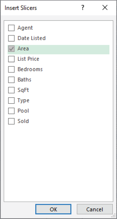
FIGURE 4.30 Use the Insert Slicers dialog box to specify which slicers to create.
Place a check mark next to the field(s) that you want to filter. You can create a slicer for each column, but that's rarely needed. In most cases, you'll want to be able to filter the table by only a few fields. Click OK, and Excel creates a slicer for each field you specified.
A slicer contains a button for every unique item in the field. In the real estate listing example, the slicer for the Agent field contains 14 buttons because the table has records for 14 different agents.
To use a slicer, just click one of the buttons. The table displays only the rows that have a value that corresponds to the button. You can also press Ctrl to select multiple buttons and press Shift to select a continuous group of buttons, which would be useful for selecting a range of List Price values. The slicer also has a multi-select button at the top. Click that button to toggle multi-select mode, and you won't have to hold down the Ctrl key.
If your table has more than one slicer, it's filtered by the selected buttons in each slicer. To remove filtering for a particular slicer, click the Clear Filter icon in the upper-right corner of the slicer.
Use the tools in the Slicer Ribbon to change the appearance or layout of a slicer. You have quite a bit of flexibility.
Figure 4.31 shows a table with two slicers. The table is filtered to show only the records for Adams, Barnes, and Chung in the Downtown area.
Changing the table's appearance
When you create a table, Excel applies the default table style. The actual appearance depends on which document theme is used in the workbook (see Chapter 5, “Formatting Worksheets”). If you prefer a different look, you can easily apply a different table style.
Select any cell in the table and choose Table Design ➪ Table Styles. The Ribbon shows one row of styles, but if you click the More button at the bottom of the scrollbar to the right, Excel displays the Table Styles gallery, as shown in Figure 4.32. The styles are grouped into three categories: Light, Medium, and Dark. Notice that you get a “live” preview as you move your mouse among the styles. When you see one you like, just click to make it permanent. And yes, some are really ugly and practically illegible.
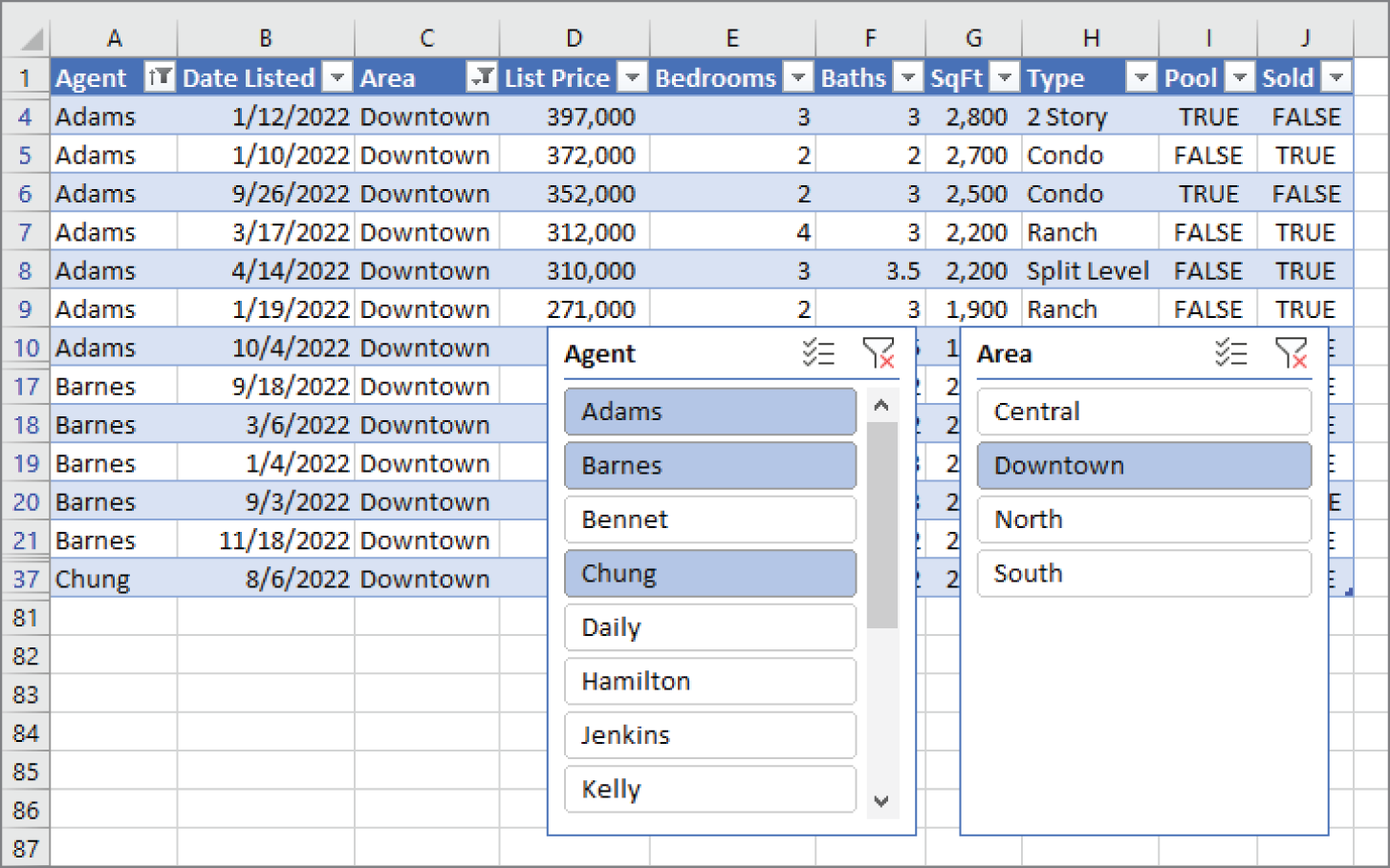
FIGURE 4.31 The table is filtered by two slicers.
For a different set of color choices, choose Page Layout ➪ Themes ➪ Themes to select a different document theme.
You can change some elements of the style by using the check box controls in the Table Design ➪ Table Style Options group. These controls determine whether various elements of the table are displayed and whether some formatting options are in effect:
- Header Row Toggles the display of the header row.
- Total Row Toggles the display of the total row.
- First Column Toggles special formatting for the first column. Depending on the table style used, this command might have no effect.
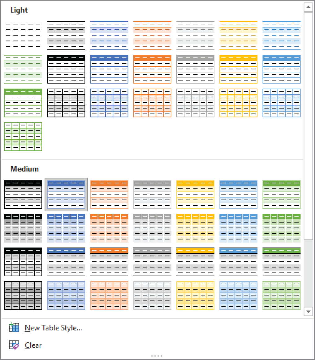
FIGURE 4.32 Excel offers many different table styles.
- Last Column Toggles special formatting for the last column. Depending on the table style used, this command might have no effect.
- Banded Rows Toggles the display of banded (alternating color) rows.
- Banded Columns Toggles the display of banded columns.
- Filter Button Toggles the display of the drop-down buttons in the table's header row.
If you'd like to create a custom table style, choose Table Design ➪ Table Styles ➪ New Table Style to display the New Table Style dialog box, shown in Figure 4.33. You can customize any or all of the 12 table elements. Select an element from the list, click Format, and specify the formatting for that element. When you're finished, give the new style a name and click OK. Your custom table style will appear in the Table Styles gallery in the Custom category.
Custom table styles are available only in the workbook in which they were created. However, if you copy a table that uses a custom style to a different workbook, the custom style will be available in the other workbook.
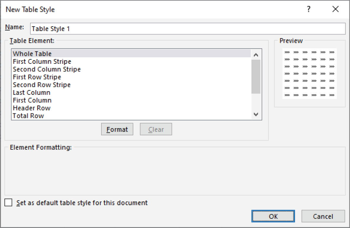
FIGURE 4.33 Use this dialog box to create a new table style.