CHAPTER 7
Printing Your Work
Despite predictions of the “paperless office,” paper remains an excellent way to carry information around and share it with others, particularly if there's no electricity or Wi-Fi where you're going. Some of the worksheets that you develop with Excel will end up as hard-copy reports, and you'll want them to look as good as possible. You'll find that printing from Excel is quite easy and that you can generate attractive, well-formatted reports with minimal effort. In addition, Excel has many options that give you a great deal of control over the printed page. We explain these options in this chapter.
Doing Basic Printing
If you want to print a copy of a worksheet with no fuss and bother, use the Quick Print option. One way to access this command is to choose File ➪ Print (which displays the Print pane of Backstage view) and then click the Print button. The keyboard shortcut Ctrl+P has the same effect as File ➪ Print. When you use Ctrl+P to show the Backstage view, the Print button has the focus, so you can simply press Enter to print.
If you like the idea of one-click printing, take a few seconds to add a new button to your Quick Access Toolbar. Click the downward-pointing arrow on the right of the Quick Access Toolbar and then choose Quick Print from the drop-down list. Excel adds the Quick Print icon to your Quick Access Toolbar.
Clicking the Quick Print button prints the current worksheet on the currently selected printer, using the default print settings. If you've changed any of the default print settings (by using the Page Layout tab), Excel uses the new settings; otherwise, it uses the following default settings:
- Prints the active worksheet (or all selected worksheets), including any embedded charts or objects
- Prints one copy
- Prints the entire active worksheet
- Prints in portrait mode
- Doesn't scale the printed output
- Uses letter-size paper with 0.75-inch margins for the top and bottom and 0.70-inch margins for the left and right margins (for the U.S. version)
- Prints with no headers or footers
- Doesn't print cell notes or comments
- Prints with no cell gridlines
- For wide worksheets that span multiple pages, prints down and then over
When you print a worksheet, Excel prints only the active area of the worksheet. In other words, it won't print all 17 billion cells—just those that have data in them. If the worksheet contains any embedded charts or other graphic objects (such as SmartArt or shapes), they're also printed.
Changing Your Page View
Page Layout view shows your worksheet divided into pages. In other words, you can visualize your printed output while you work.
Page Layout view is one of three worksheet views, which are controlled by the three icons on the right side of the status bar. You could also use the commands in the View ➪ Workbook Views group on the Ribbon to switch views. The three view options are as follows:
- Normal The default view of the worksheet. This view may or may not show page breaks.
- Page Layout Shows individual pages.
- Page Break Preview Allows you to adjust page breaks manually.
Just click one of the icons to change the view. You can also use the Zoom slider to change the magnification from 10% (a very tiny, bird's-eye view) to 400% (very large, for showing fine detail).
The following sections describe how these views can help with printing.
Normal view
Most of the time when you work in Excel, you use Normal view. Normal view can display page breaks in the worksheet. The page breaks are indicated by horizontal and vertical dotted lines. These page break lines adjust automatically if you change the page orientation, insert or delete rows or columns, change row heights, change column widths, and so on. For example, if you find that your printed output is too wide to fit on a single page, you can adjust the column widths (keeping an eye on the page break display) until the columns are narrow enough to print on one page.
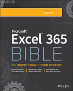
Figure 7.1 shows a part of a worksheet in Normal view, zoomed to about 50%, and with gridlines turned off. You can see the dotted line between columns D and E that indicates a page break.
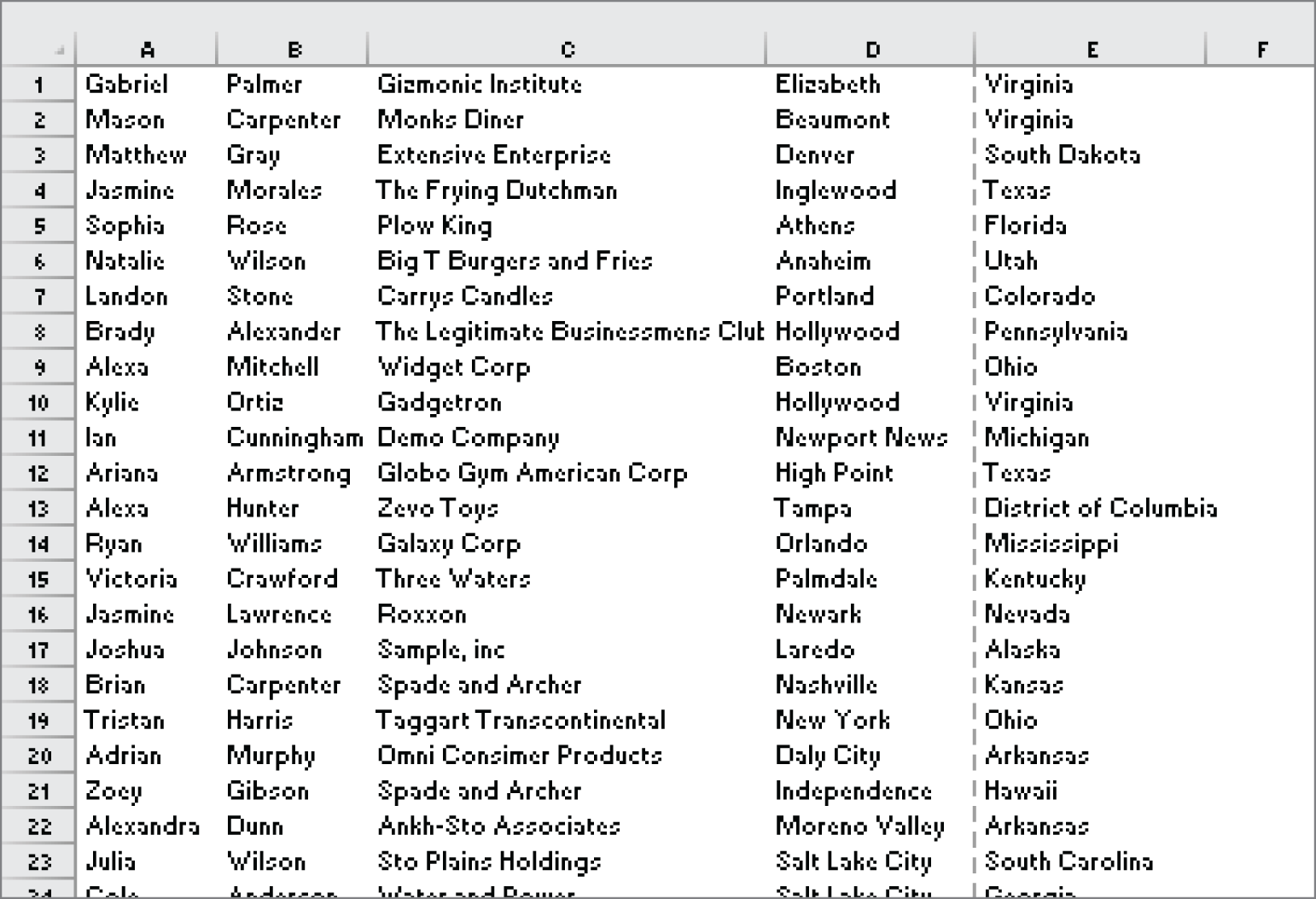
FIGURE 7.1 In Normal view, dotted lines indicate page breaks.
Page Layout view
Unlike the preview in Backstage view (choose File ➪ Print), Page Layout view is not a view-only mode. You have complete access to all Excel commands. In fact, you can use Page Layout view all the time if you like.
Figure 7.2 shows a worksheet in Page Layout view, zoomed to about 40% to show multiple pages. Contrary to Normal view, you can see the margins, the page header and footer (if any), and even some space separating each page. If you've specified any repeated rows and columns, they are also displayed—giving you a true preview of the printed output.

FIGURE 7.2 In Page Layout view, the worksheet resembles printed pages.
Page Break Preview
Page Break Preview displays the worksheet and the page breaks. Figure 7.3 shows an example. This view mode is different from Normal view mode with page breaks turned on. The key difference is that you can drag the page breaks. You can also drag the edges of the print area to change its size (if you've set a print area). Unlike Page Layout view, Page Break Preview does not display margins, headers, or footers.
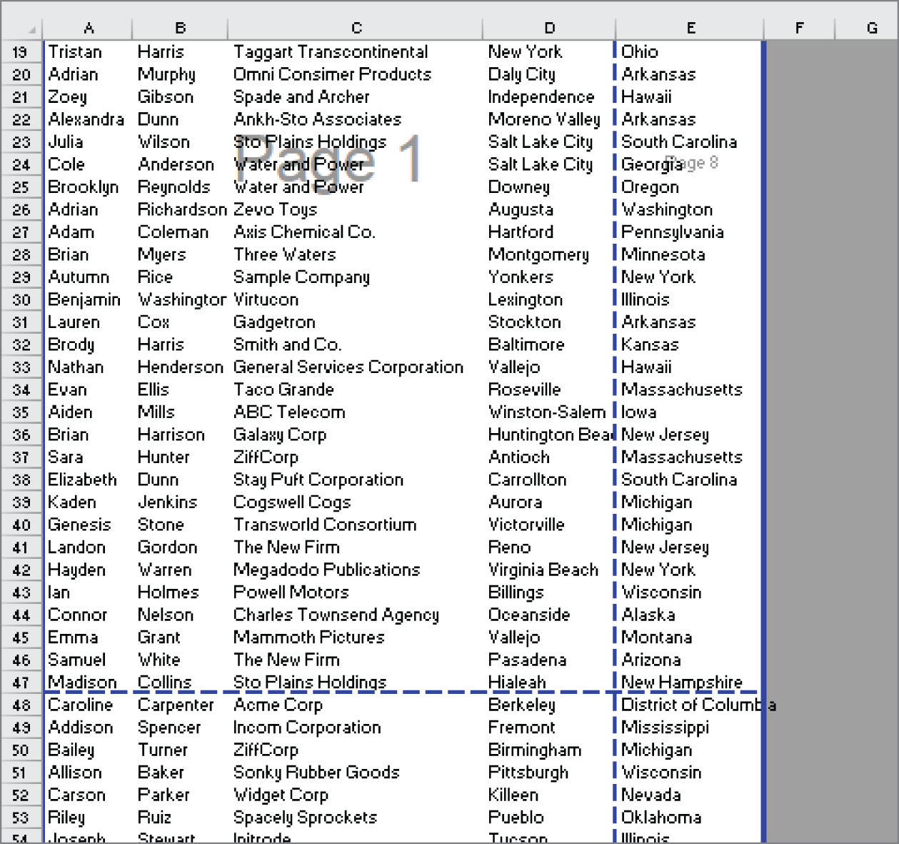
FIGURE 7.3 Page Break Preview allows you to drag page breaks and print area borders.
When you enter Page Break Preview, Excel performs the following:
- Changes the zoom factor so that you can see more of the worksheet
- Displays the page numbers overlaid on the pages
- Displays the current print range with a white background; nonprinting areas appear with a gray background
- Displays all page breaks as draggable dashed lines
When you change the page breaks by dragging, Excel automatically adjusts the scaling so that the information fits on the pages, per your specifications.
To exit Page Break Preview, just click one of the other View icons on the right side of the status bar.
Adjusting Common Page Setup Settings
Clicking the Quick Print button (or choosing File ➪ Print ➪ Print) may produce acceptable results in many cases, but a little tweaking of the print settings can often improve your printed reports. You can adjust print settings in three places:
- The Print settings screen in Backstage view, displayed when you choose File ➪ Print.
- The Page Layout tab of the Ribbon.
- The Page Setup dialog box is displayed when you click the dialog box launcher in the lower-right corner of the Page Layout ➪ Page Setup group on the Ribbon. You can also access the Page Setup dialog box from the Print settings screen in Backstage view.
Table 7.1 summarizes the locations where you can make various types of print-related adjustments in Excel.
TABLE 7.1 Where to Change Printer Settings
| Setting | Print Settings Screen | Page Layout Tab of Ribbon | Page Setup Dialog Box |
|---|---|---|---|
| Number of copies | X | ||
| Printer to use | X | ||
| What to print | X | ||
| Pages to print | X | ||
| Specify worksheet print area | X | X | |
| 1-sided or 2-sided | X | ||
| Collated | X | ||
| Orientation | X | X | X |
| Paper size | X | X | X |
| Adjust margins | X | X | X |
| Specify manual page breaks | X | ||
| Specify repeating rows or columns | X | ||
| Set print scaling | X | X | X |
| Print or hide gridlines | X | X | |
| Print or hide row and column headings | X | X | |
| Specify the first page number | X | ||
| Center output on page | X | ||
| Specify header/footers and options | X | ||
| Specify how to print cell notes or comments | X | ||
| Specify page order | X | ||
| Specify black-and-white output | X | ||
| Specify how to print error cells | X | ||
| Launch Printer Properties dialog box | X | X |
Table 7.1 might make printing seem more complicated than it really is. The key point to remember is this: if you can't find a way to make a particular adjustment, it's probably available from the Page Setup dialog box.
Choosing your printer
To switch to a different printer or output device, choose File ➪ Print, and use the drop-down control in the Printer section to select a different installed printer.
Specifying what you want to print
Sometimes you may want to print only part of the worksheet rather than the entire used area. Or you may want to reprint selected pages of a report without printing all the pages. Choose File ➪ Print and use the controls in the Settings section to specify what to print.
You have several options:
- Print Active Sheets Prints the active sheet or sheets that you selected. (This option is the default.) You can select multiple sheets to print by pressing Ctrl and clicking the sheet tabs. If you select multiple sheets, Excel begins printing each sheet on a new page.
- Print Entire Workbook Prints every sheet in the workbook, including chart sheets.
- Print Selection Prints only the range that you selected before choosing File ➪ Print.
- Print Selected Chart Appears only if a chart is selected. If this option is chosen, only the chart will be printed.
- Print Selected Table Appears only if the active cell is within a table (created by choosing Insert ➪ Tables ➪ Table) when the Print settings screen is displayed. If this option is chosen, only the table will be printed.
If your printed output uses multiple pages, you can select which pages to print by indicating the number of the first and last pages to print by using Pages controls in the Settings section. You can either use the spinner controls or type the page numbers in the text boxes.
Changing page orientation
Page orientation refers to the way output is printed on the page. Choose Page Layout ➪ Page Setup ➪ Orientation ➪ Portrait to print tall pages (the default) or Page Layout ➪ Page Setup ➪ Orientation ➪ Landscape to print wide pages. Landscape orientation is useful when you have a wide range that doesn't fit on a vertically oriented page.
If you change the orientation, the onscreen page breaks adjust automatically to accommodate the new paper orientation.
Page orientation settings are also available when you choose File ➪ Print.
Specifying paper size
Choose Page Layout ➪ Page Setup ➪ Size to specify the paper size you're using. The paper size settings are also available when you choose File ➪ Print.
Printing multiple copies of a report
Use the Copies control at the top of the Print tab in Backstage view to specify the number of copies to print. Just enter the number of copies you want and then click Print.
Adjusting the page margins
Margins are the unprinted areas along the sides, top, and bottom of a printed page. Excel provides four “quick margin” settings; you can also specify the exact margin size you require. All printed pages have the same margins. You can't specify different margins for different pages.
In Page Layout view, a ruler is displayed above the column headers and to the left of the row headers. Use your mouse to drag the margins in the ruler. Excel adjusts the page display immediately. Use the horizontal ruler to adjust the left and right margins and use the vertical ruler to adjust the top and bottom margins.
From the Page Layout ➪ Page Setup ➪ Margins drop-down list, you can select Normal, Wide, Narrow, or the Last Custom Setting if you previously customized the margins. These options are also available when you choose File ➪ Print. If none of these settings does the job, choose Custom Margins to display the Margins tab of the Page Setup dialog box, as shown in Figure 7.4.
FIGURE 7.4 The Margins tab of the Page Setup dialog box
To change a margin, click the appropriate spinner (or you can enter a value directly). The margin settings that you specify in the Page Setup dialog box will then be available in the Page Layout ➪ Page Setup ➪ Margins drop-down list, referred to as Last Custom Setting.
You can also adjust margins in the preview window in Backstage view (choose File ➪ Print). Click the Show Margins button in the bottom-right corner to display the margins in the preview pane. Then drag the margin indicators to adjust the margins.
In addition to the page margins, you can adjust the distance of the header from the top of the page and the distance of the footer from the bottom of the page. These settings should be less than the corresponding margin; otherwise, the header or footer may overlap with the printed output.
By default, Excel aligns the printed page at the top and left margins. If you want the output to be centered vertically or horizontally, select the appropriate check box in the Center on Page section of the Margins tab.
Understanding page breaks
When printing lengthy reports, controlling where pages break is often important. For example, you probably don't want a row to print on a page by itself, nor do you want a table header row to be the last line on a page. Fortunately, Excel gives you precise control over page breaks.
Excel handles page breaks automatically, but sometimes you may want to force a page break—either a vertical or a horizontal one—so that the report prints the way you want. For example, if your worksheet consists of several distinct sections, you may want to print each section on a separate sheet of paper.
Inserting a page break
To insert a horizontal page break line, select the cell that will begin the new page. Make sure you select a cell in column A, though; otherwise, you'll insert a vertical page break and a horizontal page break. For example, if you want row 14 to be the first row of a new page, select cell A14. Then choose Page Layout ➪ Page Setup ➪ Breaks ➪ Insert Page Break.
To insert a vertical page break line, select the cell that will begin the new page. In this case, though, make sure to select a cell in row 1. Choose Page Layout ➪ Page Setup ➪ Breaks ➪ Insert Page Break to create the page break.
Removing manual page breaks
To remove a page break that you've added, select a cell in the first row beneath (or the first column to the right of) the manual page break and then choose Page Layout ➪ Page Setup ➪ Breaks ➪ Remove Page Break.
To remove all manual page breaks in the worksheet, choose Page Layout ➪ Page Setup ➪ Breaks ➪ Reset All Page Breaks.
Printing row and column titles
If your worksheet is set up with titles in the first row and descriptive names in the first column, it can be difficult to identify data that appears on printed pages where those titles don't appear. To resolve this problem, you can choose to print selected rows or columns as titles on each page of the printout.
Row and column titles serve pretty much the same purpose on a printout as frozen panes do in navigating within a worksheet. Keep in mind, however, that these features are independent of each other. In other words, freezing panes doesn't affect the printed output.
You can specify rows to repeat at the top of every printed page or columns to repeat at the left of every printed page. To do so, choose Page Layout ➪ Page Setup ➪ Print Titles. Excel displays the Sheet tab of the Page Setup dialog box, as shown in Figure 7.5.
Figure 7.5 shows that row 1 will repeat at the top of the page and columns A and B will repeat on the left of the page. Even if you only want one row or column, you have to include the colon. To set these properties, activate the appropriate box (either Rows to Repeat at Top or Columns to Repeat at Left) and then select the rows or columns in the worksheet. Or you can enter these references manually. For example, to specify rows 1 and 2 as repeating rows, enter 1:2.

FIGURE 7.5 Use the Sheet tab of the Page Setup dialog box to specify rows or columns that will appear on each printed page.
Scaling printed output
In some cases, you may need to force your printed output to fit on a specific number of pages. You can do so by enlarging or reducing the size. To enter a scaling factor, choose Page Layout ➪ Scale to Fit ➪ Scale. You can scale the output from 10% up to 400%. To return to normal scaling, enter 100%.
To force Excel to print using a specific number of pages, choose Page Layout ➪ Scale to Fit ➪ Width and Page Layout ➪ Scale to Fit ➪ Height. When you change either one of these settings, the corresponding scale factor is displayed in the Scale control.
Printing cell gridlines
Typically, cell gridlines aren't printed. If you want your printout to include the gridlines, choose Page Layout ➪ Sheet Options ➪ Gridlines ➪ Print.
Alternatively, you can insert borders around some cells to simulate gridlines. Change the border color to White, Background 1, 25% Darker to get a pretty good simulation of a gridline. To change the color, choose Home ➪ Font ➪ Borders ➪ More Borders. Make sure you change the color before you apply the border.
Printing row and column headers
By default, row and column headers for a worksheet are not printed. If you want your printout to include these items, choose Page Layout ➪ Sheet Options ➪ Headings ➪ Print.
Using a background image
Would you like to have a background image on your printouts? Unfortunately, you can't. You may have noticed the Page Layout ➪ Page Setup ➪ Background command. This button displays a dialog box that lets you select an image to display as a background. Placing this control among the other print-related commands is misleading. Background images placed on a worksheet are never printed.
Adding a Header or a Footer to Your Reports
A header is information that appears at the top of each printed page. A footer is information that appears at the bottom of each printed page. By default, new workbooks have space for headers or footers but nothing in them.
You can specify headers and footers by using the Header/Footer tab of the Page Setup dialog box. Or you can simplify the task by switching to Page Layout view, where you can click the section labeled Add Header or Add Footer.
You can then type the information and apply any type of formatting you like. Note that headers and footers consist of three sections: left, center, and right. For example, you can create a header that prints your name at the left margin, the worksheet name centered in the header, and the page number at the right margin.
When you activate the header or footer section in Page Layout view, the Ribbon displays a new contextual tab: Header & Footer. Use the controls on this tab to work with headers and footers.
Selecting a predefined header or footer
You can choose from a number of predefined headers or footers by using either of the two drop-down lists in the Header & Footer ➪ Header & Footer group. Notice that some items in these lists consist of multiple parts, separated by a comma. Each part goes into one of the three header or footer sections (left, center, or right). Figure 7.6 shows an example of a header that uses all three sections.
Understanding header and footer element codes
When a header or footer section is activated, you can type whatever text you like into the section. Or to insert variable information, you can insert any of several element codes by clicking a button in the Header & Footer ➪ Header & Footer Elements group. Each button inserts a code into the selected section. For example, to insert the current date, click the Current Date button. Table 7.2 lists the buttons and their functions.
TABLE 7.2 Header and Footer Buttons and Their Functions
| Button | Code | Function |
|---|---|---|
| Page Number |
&[Page]
| Displays the page number |
| Number of Pages |
&[Pages]
| Displays the total number of pages to be printed |
| Current Date |
&[Date]
| Displays the current date |
| Current Time |
&[Time]
| Displays the current time |
| File Path |
&[Path]&[File]
| Displays the workbook's complete path and filename |
| File Name |
&[File]
| Displays the workbook name |
| Sheet Name |
&[Tab]
| Displays the sheet's name |
| Picture |
&[Picture]
| Enables you to add a picture |
| Format Picture | Not applicable | Enables you to change an added picture's settings |
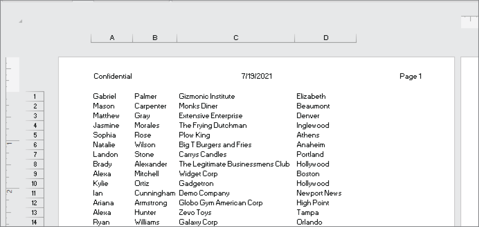
FIGURE 7.6 This three-part header is one of Excel's predefined headers.
You can combine text and codes and insert as many codes as you like into each section.
You can also use different fonts and sizes in your headers and footers. Just select the text you want to change and then use the formatting tools in the Home ➪ Font group. Or use the controls on the Mini toolbar, which appears automatically when you select the text. If you don't change the font, Excel uses the font defined for the Normal style.
Unfortunately, you can't print the contents of a specific cell in a header or footer. For example, you may want Excel to use the contents of cell A1 as part of a header. To do so, you need to enter the cell's contents manually—or write a VBA macro to perform this operation before the sheet is printed.
Exploring other header and footer options
When a header or footer is selected in Page Layout view, the Header & Footer ➪ Options group contains controls that let you specify other options:
- Different First Page If this option is checked, you can specify a different header/footer for the first printed page.
- Different Odd & Even Pages If this option is checked, you can specify a different header/footer for odd and even pages.
- Scale with Document If this option is checked, the font size in the header and footer will be sized accordingly if the document is scaled when printed. This option is enabled by default.
- Align with Page Margins If this option is checked, the left header and footer will be aligned with the left margin, and the right header and footer will be aligned with the right margin. This option is enabled by default.
Exploring Other Print-Related Topics
The following sections cover some additional topics related to printing from Excel.
Copying Page Setup settings across sheets
Each Excel worksheet has its own print setup options (orientation, margins, headers and footers, and so on). These options are specified in the Page Setup group of the Page Layout tab.
When you add a new sheet to a workbook, it contains the default page setup settings. Here's an easy way to transfer the settings from one worksheet to additional worksheets:
- Activate the sheet that contains the desired setup information. This is the source sheet.
- Select the target sheets, and Ctrl+click the sheet tabs of the sheets that you want to update with the settings from the source sheet.
- Click the dialog box launcher in the lower-right corner of the Page Layout ➪ Page Setup group.
- When the Page Setup dialog box appears, click OK to close it.
- Ungroup the sheets by right-clicking any selected sheet and choosing Ungroup Sheets from the shortcut menu. Because multiple sheets are selected when you close the Page Setup dialog box, the settings of the source sheet will be transferred to all target sheets.
Preventing certain cells from being printed
If your worksheet contains confidential information, you may want to print the worksheet but not the confidential parts. You can use several techniques to prevent certain parts of a worksheet from printing:
- Hide rows or columns When you hide rows or columns, the hidden rows or columns aren't printed. Choose Home ➪ Cells ➪ Format drop-down list to hide the selected rows or columns.
- Hide cells or ranges by making the text color the same color as the background color You can hide cells or ranges by making the text color the same color as the background color. Be aware, however, that this method may not work for all printers.
- Hide cells or ranges by using a custom number format You can hide cells by using a custom number format that consists of three semicolons (
;;;). See Chapter 2, “Entering and Editing Worksheet Data,” for more information about using custom number formats. - Mask an area You can mask a confidential area of a worksheet by covering it with a rectangle shape. Choose Insert ➪ Illustrations ➪ Shapes and click the Rectangle shape. You'll probably want to adjust the fill color to match the cell background and remove the border.
If you find that you must regularly hide data before you print certain reports, consider using the Custom Views feature, discussed later in this chapter. (See “Creating custom views of your worksheet.”) This feature allows you to create a named view that doesn't show the confidential information.
Preventing objects from being printed
To prevent objects on the worksheet (such as charts, shapes, and SmartArt) from being printed, you need to access the Properties tab of the object's Format task pane (see Figure 7.7):
- Right-click the object and choose Format xxxx from the shortcut menu. (xxxx varies, depending on the object.)
- In the Format task pane that opens for the object, click the Size & Properties icon.
- Expand the Properties section of the task pane.
- Remove the check mark for Print Object.

FIGURE 7.7 Use the Properties section in the object's Format task pane to prevent objects from printing.
Creating custom views of your worksheet
If you need to create several different printed reports from the same Excel workbook, setting up the specific settings for each report can be a tedious job. For example, you may need to print a full report in landscape mode for your boss. Another department may require a simplified report using the same data but with some hidden columns in portrait mode. You can simplify the process by creating custom named views of your worksheets that include the proper settings for each report.
The Custom Views feature enables you to give names to various views of your worksheet. You can quickly switch among these named views. A view includes settings for the following:
- Print settings, as specified in the Page Layout ➪ Page Setup, Page Layout ➪ Scale to Fit, and Page Layout ➪ Sheet Options groups
- Hidden rows and columns
- The worksheet view (Normal, Page Layout, Page Break Preview)
- Selected cells and ranges
- The active cell
- The zoom factor
- Window sizes and positions
- Frozen panes
If you find that you're constantly fiddling with these settings before printing and then changing them back, using custom named views can save you some work.
To create a named view, follow these steps:
- Set up the view settings the way you want them. For example, hide some columns.
- Choose View ➪ Workbook Views ➪ Custom Views. The Custom Views dialog box appears.
- Click the Add button. The Add View dialog box (shown in Figure 7.8) appears.

FIGURE 7.8 Use the Add View dialog box to create a named view.
- Provide a descriptive name. You can also specify what to include in the view by using the two check boxes. For example, if you don't want the view to include print settings, remove the check mark from Print Settings.
- Click OK to save the named view.
Then when you're ready to print, open the Custom Views dialog box to see all named views. To select a particular view, just select it from the list and click the Show button. To delete a named view from the list, click the Delete button.
Creating PDF files
The PDF file format is widely used as a way to present information in a read-only manner with precise control over the layout. If you need to share your work with someone who doesn't have Excel, creating a PDF is often a good solution. Free software to display PDFs is available from a number of sources.
XPS is another “electronic paper” format, developed by Microsoft as an alternative to the PDF format. Currently, there is little third-party support for the XPS format.
To save a worksheet in PDF or XPS format, choose File ➪ Export ➪ Create PDF/XPS Document ➪ Create PDF/XPS. Excel displays the Publish as PDF or XPS dialog box, in which you can specify a filename and location and set some other options.