CHAPTER 5
Formatting Worksheets
Formatting your worksheet is more than just making your worksheet pretty. Proper formatting can help users understand the purpose of the worksheet and help prevent data entry errors.
Stylistic formatting isn't essential for every workbook that you develop, especially if it's only for your own use. On the other hand, it takes only a few moments to apply some simple formatting, and after you apply it, the formatting will remain in place without further effort on your part.
Getting to Know the Formatting Tools
Figure 5.1 shows how even simple formatting can significantly improve a worksheet's readability. The unformatted worksheet (on the left) is perfectly functional but not very readable compared to the formatted worksheet (on the right).
The Excel cell formatting tools are available in three locations.
- On the Home tab of the Ribbon
- On the Mini toolbar that appears when you right-click a selected range or a cell
- From the Format Cells dialog box

FIGURE 5.1 Simple formatting can greatly improve the appearance of your worksheet.
In addition, many common formatting commands have keyboard shortcuts.
Using the formatting tools on the Home tab
The Home tab of the Ribbon provides quick access to the most commonly used formatting options. Start by selecting the cell or range you want to format. Then use the appropriate tool in the Font, Alignment, or Number group.
Using these tools is intuitive, and the best way to familiarize yourself with them is to experiment. Enter some data, select some cells, and then click the controls to change the appearance. Note that some of these controls are actually drop-down lists. Click the small arrow on the button, and the button expands to display your choices.
Using the Mini toolbar
When you right-click a cell or a range selection, you get a shortcut menu. In addition, the Mini toolbar appears above or below the shortcut menu. Figure 5.2 shows how this toolbar looks. The Mini toolbar for cell formatting contains the most commonly used controls from the Home tab of the Ribbon.

FIGURE 5.2 The Mini toolbar appears above or below the right-click shortcut menu.
If you use a tool on the Mini toolbar, the shortcut menu disappears, but the toolbar remains visible so that you can apply other formatting to the selected cells. To hide the Mini toolbar, just click in any cell or press Esc.
Using the Format Cells dialog box
The formatting controls available on the Home tab of the Ribbon are sufficient most of the time, but some types of formatting require that you use the Format Cells dialog box. This tabbed dialog box lets you apply nearly any type of stylistic formatting and number formatting. The formats that you choose in the Format Cells dialog box apply to the selected cells. Later sections in this chapter cover some of the tabs of the Format Cells dialog box.
After selecting the cell or range to format, you can display the Format Cells dialog box by using any of the following methods:
- Press Ctrl+1.
- Click the dialog box launcher in Home ➪ Font, Home ➪ Alignment, or Home ➪ Number. (The dialog box launcher is the small downward-pointing arrow icon displayed to the right of the group name in the Ribbon.) When you display the Format Cells dialog box using a dialog box launcher, the dialog box is displayed with the appropriate tab visible.
- Right-click the selected cell or range and choose Format Cells from the shortcut menu.
- Click the More command in some of the drop-down controls in the Ribbon. For example, the Home ➪ Font ➪ Border drop-down includes an item named More Borders.
The Format Cells dialog box contains six tabs: Number, Alignment, Font, Border, Fill, and Protection. The following sections contain more information about the formatting options available in this dialog box.
Formatting Your Worksheet
Excel offers most of the same formatting options as other Office applications like Word or PowerPoint. As you might expect, cell-related formatting like fill color and borders feature more prominently in Excel than some of the other applications.
Using fonts to format your worksheet
You can use different fonts, font sizes, or text attributes in your worksheets to make various parts stand out, such as the headers for a table. You also can adjust the font size. For example, using a smaller font allows for more information on a single screen or printed page.
By default, Excel uses the 11-point (pt) Calibri font. A font is described by its typeface (Calibri, Cambria, Arial, Times New Roman, Courier New, and so on) as well as by its size, measured in points. (Seventy-two points equal one inch.) Excel's row height, by default, is 15 pt. Therefore, 11-pt type entered into 15-pt rows leaves a small amount of blank space between the characters in vertically adjacent rows.
Use the Font and Font Size tools in the Font group on the Home tab of the Ribbon (or on the Mini toolbar) to change the font or size for selected cells.
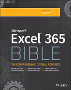
You also can use the Font tab in the Format Cells dialog box to choose fonts, as shown in Figure 5.3. This tab enables you to control several other font attributes that aren't available elsewhere. Besides choosing the font and font size, you can change the font style (bold, italic), underlining, color, and effects (strikethrough, superscript, or subscript). If you select the Normal Font check box, Excel displays the selections for the font defined for the Normal style. We discuss styles later in this chapter (see “Using Named Styles for Easier Formatting”).
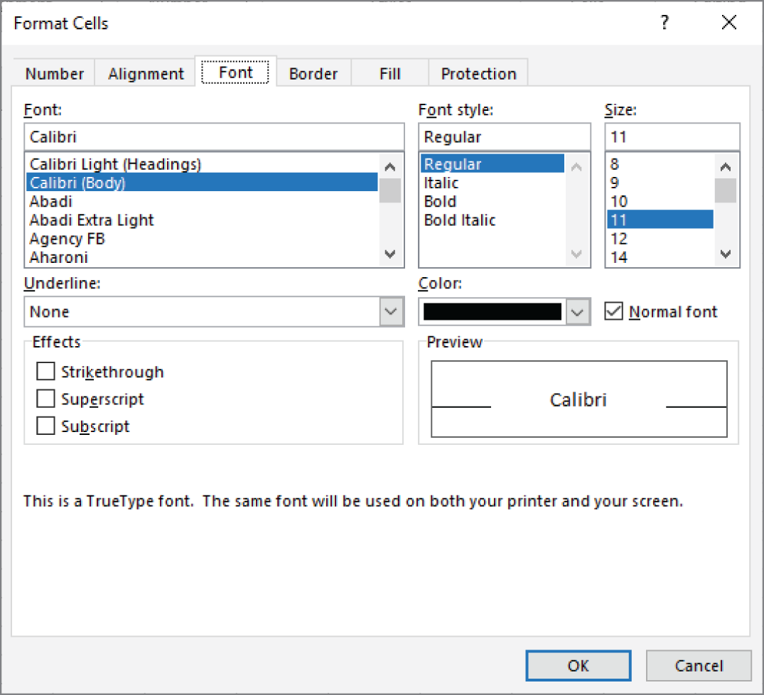
FIGURE 5.3 The Font tab of the Format Cells dialog box gives you many additional font attribute options.
Figure 5.4 shows several examples of font formatting. In this figure, gridlines were turned off to make the underlining more visible. Notice, in the figure, that Excel provides four different underlining styles. In the two nonaccounting underline styles, only the cell contents are underlined. In the two accounting underline styles, the entire width of the cells is always underlined.
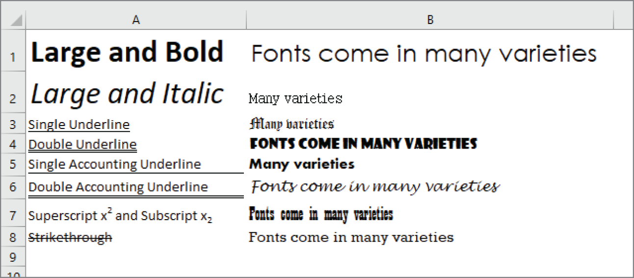
FIGURE 5.4 You can choose many different font formatting options for your worksheets.
If you prefer to keep both hands on the keyboard, you can use the following shortcut keys to format a selected range quickly:
- Ctrl+B: Bold
- Ctrl+I: Italic
- Ctrl+U: Underline
- Ctrl+5: Strikethrough
These shortcut keys act as a toggle. For example, you can turn bold on and off by repeatedly pressing Ctrl+B.
Changing text alignment
The contents of a cell can be aligned horizontally and vertically. By default, Excel aligns numbers to the right and text to the left. All cells use bottom alignment by default.
Overriding these defaults is a simple matter. The most commonly used alignment commands are in the Alignment group on the Home tab of the Ribbon. Use the Alignment tab of the Format Cells dialog box for even more options (see Figure 5.5).
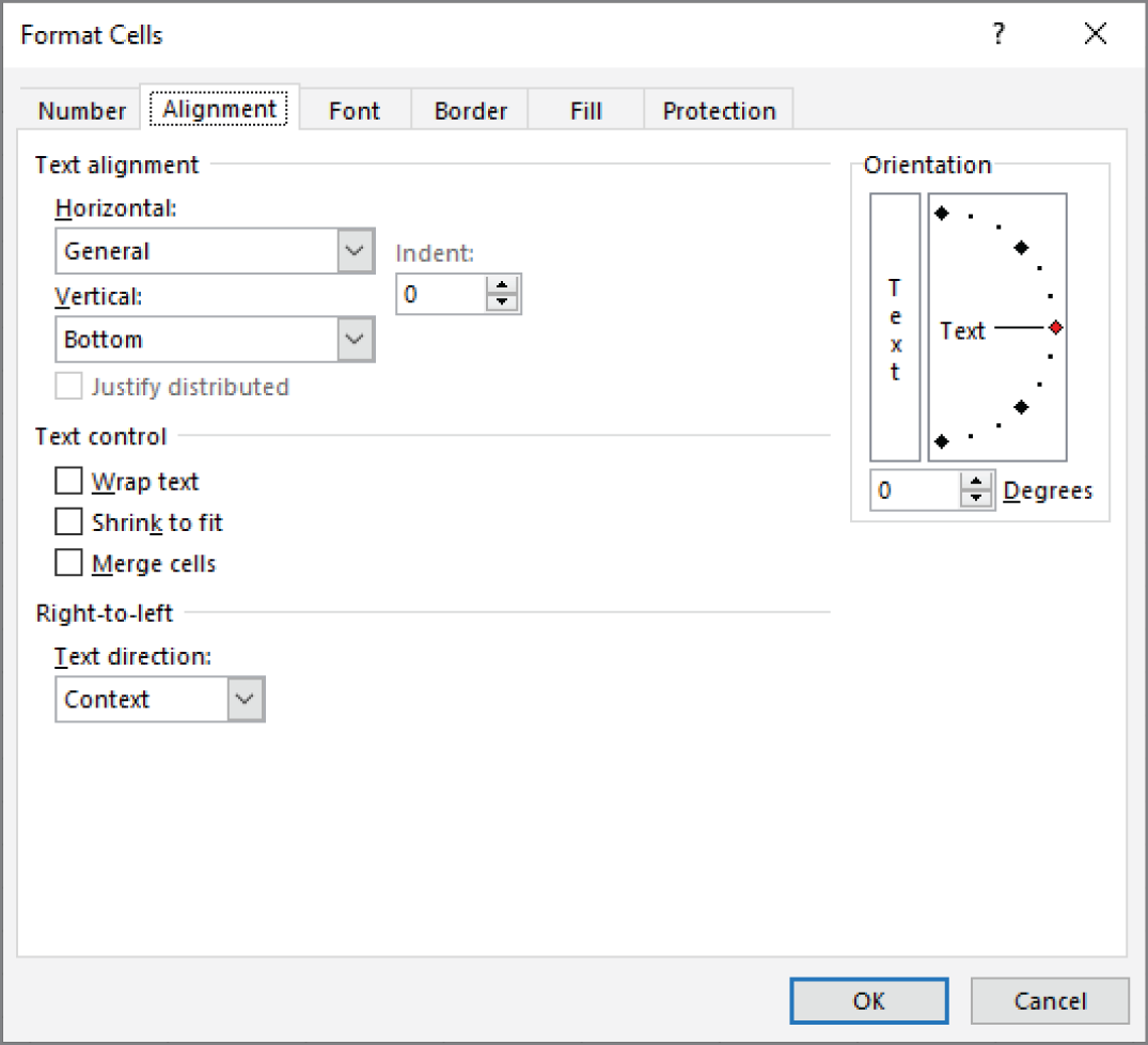
FIGURE 5.5 The full range of alignment options is available on the Alignment tab of the Format Cells dialog box.
Choosing horizontal alignment options
Horizontal alignment options, which control how cell contents are distributed across the width of the cell (or cells), are available from the Format Cells dialog box.
- General Aligns numbers to the right, aligns text to the left, and centers logical and error values. This option is the default horizontal alignment.
- Left Aligns the cell contents to the left side of the cell. If the text is wider than the cell, the text spills over to the cell on the right. If the cell on the right isn't empty, the text is truncated and not completely visible. This is also available on the Ribbon.
- Center Centers the cell contents in the cell. If the text is wider than the cell, the text spills over to cells on either side if they're empty. If the adjacent cells aren't empty, the text is truncated and not completely visible. This is also available on the Ribbon.
- Right Aligns the cell contents to the right side of the cell. If the text is wider than the cell, the text spills over to the cell on the left. If the cell on the left isn't empty, the text is truncated and not completely visible. This is also available on the Ribbon.
- Fill Repeats the contents of the cell until the cell's width is filled. If cells to the right also are formatted with Fill alignment, they also are filled.
- Justify Justifies the text to the left and right of the cell. This option is applicable only if the cell is formatted as wrapped text and uses more than one line.
- Center Across Selection Centers the text over the selected columns. This option is useful for centering a heading over several columns.
- Distributed Distributes the text evenly across the cell, adding additional white space between words where necessary.
Figure 5.6 shows examples of text that uses three types of horizontal alignment: Left, Justify, and Distributed (with an indent).
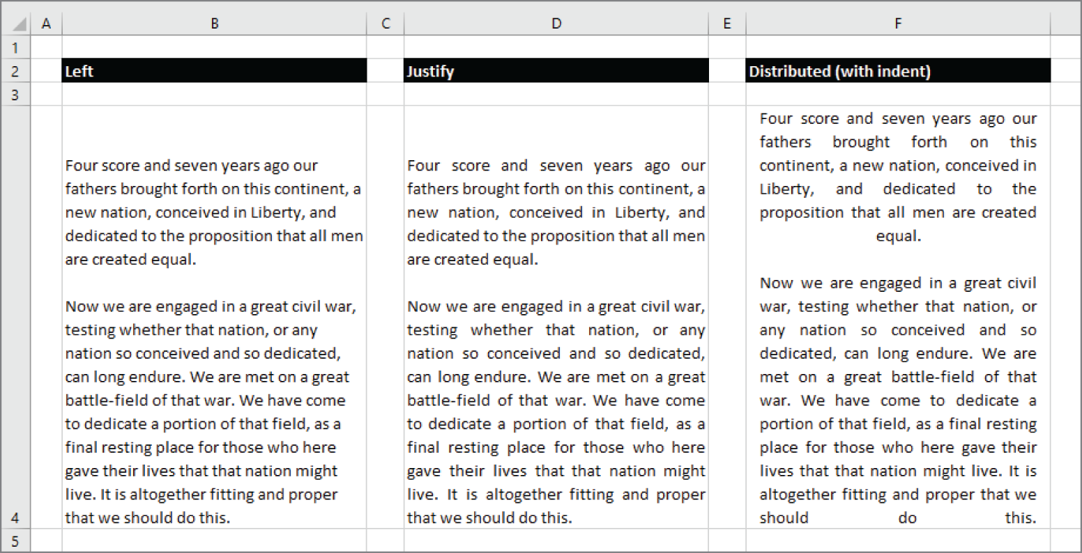
FIGURE 5.6 The same text, displayed with three types of horizontal alignment
Choosing vertical alignment options
Vertical alignment options typically aren't used as often as horizontal alignment options. In fact, these settings are useful only if you've adjusted row heights so that they're considerably taller than normal.
Here are the vertical alignment options available in the Format Cells dialog box:
- Top Aligns the cell contents to the top of the cell. This is also available on the Ribbon.
- Center Centers the cell contents vertically in the cell. This is also available on the Ribbon.
- Bottom Aligns the cell contents to the bottom of the cell. This is also available on the Ribbon. This option is the default vertical alignment.
- Justify Justifies the text vertically in the cell; this option is applicable only if the cell is formatted as wrapped text and uses more than one line. This setting can be used to increase the line spacing.
- Distributed Distributes the text evenly between the top and bottom of the cell, adding additional white space between lines where necessary. If there is only one line of text in the cell, it's identical to the Center option.
Wrapping or shrinking text to fit the cell
If you have text too wide to fit the column width but you don't want that text to spill over into adjacent cells, you can use either the Wrap Text option or the Shrink to Fit option to accommodate that text. The Wrap Text option is also available on the Ribbon.
The Wrap Text option displays the text on multiple lines in the cell, if necessary. Use this option to display lengthy headings without having to make the columns too wide and without reducing the size of the text.
The Shrink to Fit option reduces the size of the text so that it fits into the cell without spilling over to the next cell. The times that this command is useful seem to be rare. Unless the text is just slightly too long, the result is almost always illegible.
Merging worksheet cells to create additional text space
A handy formatting option is the ability to merge two or more cells. When you merge cells, you don't combine the contents of cells. Rather, you combine a group of cells into a single cell that occupies the same space. The worksheet shown in Figure 5.7 contains four sets of merged cells. Range C2:I2 has been merged into a single cell and so have ranges J2:P2, B4:B8, and B9:B13. In the latter two cases, the text orientation has also been changed (see “Displaying text at an angle” later in this chapter).
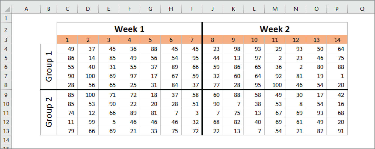
FIGURE 5.7 Merge worksheet cells to make them act as if they were a single cell.
You can merge any number of cells occupying any number of rows and columns. In fact, you can merge all 17 billion cells in a worksheet into a single cell—although there probably isn't a good reason to do so, except maybe to play a trick on a co-worker.
The range that you intend to merge should be empty, except for the upper-left cell. If any of the other cells that you intend to merge are not empty, Excel displays a warning. If you continue, all the data (except in the upper-left cell) will be deleted.
You can use the Alignment tab of the Format Cells dialog box to merge cells, but using the Merge & Center control in the Alignment group on the Ribbon (or on the Mini toolbar) is simpler. To merge cells, select the cells that you want to merge and then click the Merge & Center button. The cells will be merged, and the content in the upper-left cells will be centered horizontally. The Merge & Center button acts as a toggle. To unmerge cells, select the merged cells and click the Merge & Center button again.
After you merge cells, you can change the alignment to something other than Center by using the controls in the Home ➪ Alignment group.
The Home ➪ Alignment ➪ Merge & Center control contains a drop-down list with these additional options:
- Merge Across When a multirow range is selected, this command creates multiple merged cells—one for each row.
- Merge Cells Merges the selected cells without applying the Center attribute.
- Unmerge Cells Unmerges the selected cells.
Displaying text at an angle
In some cases, you may want to create more visual impact by displaying text at an angle within a cell. You can display text horizontally, vertically, or at any angle between 90 degrees up and 90 degrees down.
From the Home ➪ Alignment ➪ Orientation drop-down list, you can apply the most common text angles. For more control, use the Alignment tab of the Format Cells dialog box. In the Format Cells dialog box (refer to Figure 5.5), use the Degrees spinner control—or just drag the red pointer in the gauge. You can specify a text angle between –90 and +90 degrees.
Figure 5.8 shows an example of text displayed at a 45-degree angle.
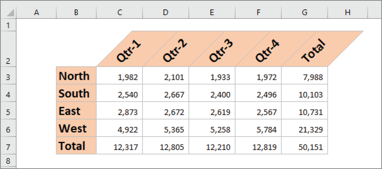
FIGURE 5.8 Rotate text for additional visual impact.
Using colors and shading
Excel provides the tools to create some colorful worksheets. You can change the color of the text or add colors to the backgrounds of the worksheet cells. Prior to Excel 2007, workbooks were limited to a palette of 56 colors. Since then, Microsoft has increased the number of colors to more than 16 million.
You control the color of the cell's text by choosing Home ➪ Font ➪ Font Color. Control the cell's background color by choosing Home ➪ Font ➪ Fill Color. Both of these color controls are also available on the Mini toolbar, which appears when you right-click a cell or range.
Even though you have access to a lot of colors, you might want to stick with the 10 theme colors (and their light/dark variations) displayed in the various color selection controls. In other words, avoid using the More Colors option, which lets you select a color. Why? First, those 10 colors were chosen because they “go together.” (Well, at least somebody thought they did.) Another reason involves document themes. If you switch to a different document theme for your workbook, nontheme colors aren't changed. In some cases, the result may be less than pleasing aesthetically. (See “Understanding Document Themes” later in this chapter for more information about themes.)
Adding borders and lines
Borders (and lines within the borders) are another visual enhancement that you can add around groups of cells. Borders are often used to group a range of similar cells or to delineate rows or columns. Excel offers 13 preset styles of borders, as you can see in the Home ➪ Font ➪ Borders drop-down list shown in Figure 5.9. This control works with the selected cell or range and enables you to specify which, if any, border style to use for each border of the selection.
You may prefer to draw borders rather than select a preset border style. To do so, use the Draw Border or Draw Border Grid command from the Home ➪ Font ➪ Borders drop-down list. Selecting either command lets you create borders by dragging your mouse. Use the Line Color or Line Style command to change the color or style. When you're finished drawing borders, press Esc to cancel the border-drawing mode.
Another way to apply borders is to use the Border tab of the Format Cells dialog box, which is shown in Figure 5.10. One way to display this dialog box is to select More Borders from the Borders drop-down list.
Before you display the Format Cells dialog box, select the cell or range to which you want to add borders. Then, in the Format Cells dialog box, choose a line style and color and then choose the border position for the line style by clicking one or more of the Border icons. (These icons are toggles.)
Notice that the Border tab has three preset icons, which can save you some clicking. If you want to remove all borders from the selection, click None. To put an outline around the selection, click Outline. To put borders inside the selection, click Inside.
Excel displays the selected border style in the dialog box; there is no live preview in the worksheet. You can choose different styles for different border positions; you can also choose a color for the border. Using this dialog box may require some experimentation, but you'll get the hang of it.
When you apply two diagonal lines, the cells look like they've been crossed out.
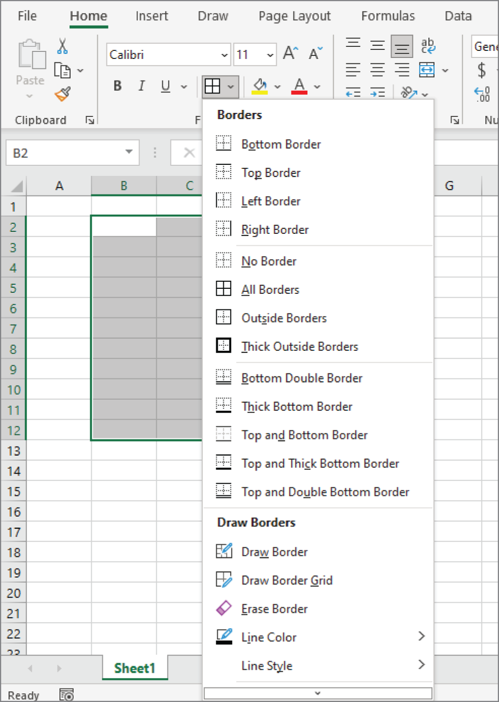
FIGURE 5.9 Use the Borders drop-down list to add lines around worksheet cells.
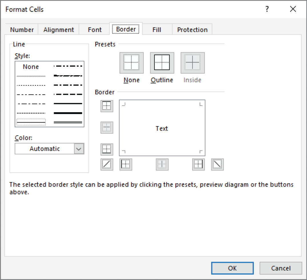
FIGURE 5.10 Use the Border tab of the Format Cells dialog box for more control over cell borders.
Using Conditional Formatting
You can apply conditional formatting to a cell so that the cell looks different depending on its contents. Conditional formatting is a useful tool for visualizing numeric data. In some cases, conditional formatting may be a viable alternative to creating a chart.
Conditional formatting lets you apply cell formatting selectively and automatically, based on the contents of the cells. For example, you can apply conditional formatting in such a way that all negative values in a range have a light-yellow background color. When you enter or change a value in the range, Excel examines the value and checks the conditional formatting rules for the cell. If the value is negative, the background is shaded; otherwise, no formatting is applied.
Specifying conditional formatting
To apply a conditional formatting rule to a cell or range, select the cells and then use one of the commands from the Home ➪ Styles ➪ Conditional Formatting drop-down list to specify a rule. The choices are as follows:
- Highlight Cells Rules Examples include highlighting cells that are greater than a particular value, are between two values, contain a specific text string, contain a date, or are duplicated.
- Top/Bottom Rules Examples include highlighting the top 10 items, the items in the bottom 20 percent, and the items that are above average.
- Data Bars Applies graphic bars directly in the cells, proportional to the cell's value.
- Color Scales Applies background color, proportional to the cell's value.
- Icon Sets Displays icons directly in the cells. The icons depend on the cell's value.
- New Rule Enables you to specify other conditional formatting rules, including rules based on a logical formula.
- Clear Rules Deletes all the conditional formatting rules from the selected cells.
- Manage Rules Displays the Conditional Formatting Rules Manager dialog box in which you create new conditional formatting rules, edit rules, or delete rules.
Using graphical conditional formats
The following sections describe the three conditional formatting options that display graphics: data bars, color scales, and icon sets. These types of conditional formatting can be useful for visualizing the values in a range.
Using data bars
The data bars conditional format displays horizontal bars directly in the cell. The length of the bar is based on the value of the cell relative to the other values in the range.
Figure 5.11 shows an example of data bars. It's a list of tracks on 39 Bob Dylan albums, with the length of each track in column D. With data bar conditional formatting applied to column D, you can tell at a glance which tracks are longer.

FIGURE 5.11 The length of the data bars is proportional to the track length in the cell in column D.
Excel provides quick access to 12 data bar styles via Home ➪ Styles ➪ Conditional Formatting ➪ Data Bars. For additional choices, click the More Rules option, which displays the New Formatting Rule dialog box. Use this dialog box to do the following:
- Show the bar only. (Hide the numbers.)
- Specify Minimum and Maximum values for the scaling.
- Change the appearance of the bars.
- Specify how negative values and the axis are handled.
- Specify the direction of the bars.
Using color scales
The color scale conditional formatting option varies the background color of a cell based on the cell's value relative to other cells in the range.
Figure 5.12 shows examples of color scale conditional formatting. The example on the left depicts monthly sales for three regions. Conditional formatting was applied to the range B4:D15. The conditional formatting uses a three-color scale, with red for the lowest value, yellow for the midpoint, and green for the highest value. Values in between are displayed using a color within the gradient. It's clear that the Central region consistently has lower sales volumes, but the conditional formatting doesn't help identify monthly differences for a particular region.
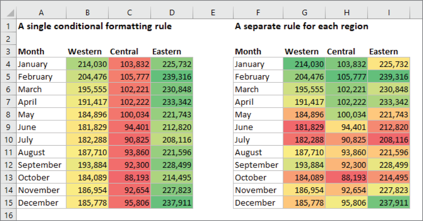
FIGURE 5.12 Two examples of color scale conditional formatting
The example on the right shows the same data, but conditional formatting was applied to each region separately. This approach facilitates comparisons within a region and can identify high or low sales months.
Neither one of these approaches is necessarily better. The way you set up conditional formatting depends entirely on what you're trying to visualize.
Excel provides six two-color scale presets and six three-color scale presets, which you can apply to the selected range by choosing Home ➪ Styles ➪ Conditional Formatting ➪ Color Scales.
To customize the colors and other options, choose Home ➪ Styles ➪ Conditional Formatting ➪ Color Scales ➪ More Rules, and the New Formatting Rule dialog box, shown in Figure 5.13, appears. Adjust the settings and watch the Preview box to see the effects of your changes.
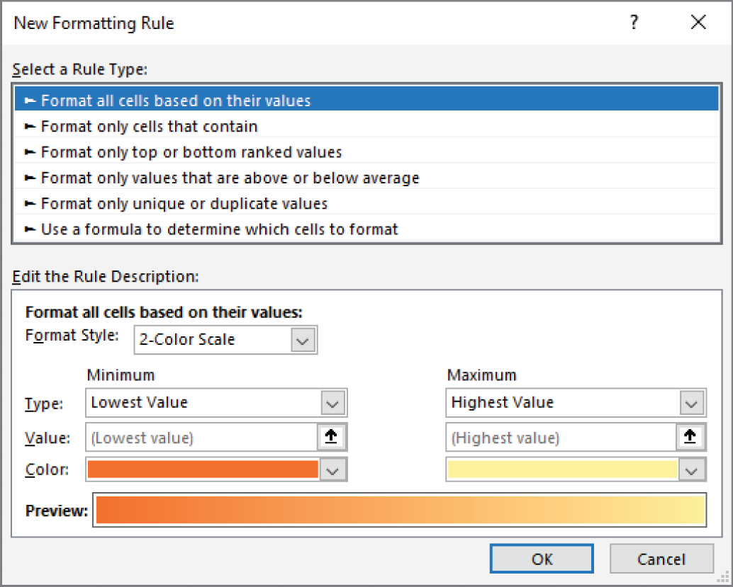
FIGURE 5.13 Use the New Formatting Rule dialog box to customize a color scale.
Using icon sets
Yet another conditional formatting option is to display an icon in the cell. The icon displayed depends on the value of the cell.
To assign an icon set to a range, select the cells and choose Home ➪ Styles ➪ Conditional Formatting ➪ Icon Sets. Excel provides 20 icon sets from which you may choose. The number of icons in the sets ranges from three to five. You can't create a custom icon set.
Figure 5.14 shows an example that uses an icon set. The symbols graphically depict the status of each project, based on the value in column C.

FIGURE 5.14 Using an icon set to indicate the status of projects
By default, the symbols are assigned using percentiles. For a three-symbol set, the items are grouped into three percentiles. For a four-symbol set, they're grouped into four percentiles. For a five-symbol set, the items are grouped into five percentiles.
If you would like more control over how the icons are assigned, choose Home ➪ Styles ➪ Conditional Formatting ➪ Icon Sets ➪ More Rules to display the New Formatting Rule dialog box. To modify an existing rule, choose Home ➪ Styles ➪ Conditional Formatting ➪ Manage Rules. Then select the rule to modify and click the Edit Rule button.
Figure 5.15 shows how to modify the icon set rules such that only projects that are 100 percent complete get the check mark icons. Projects that are 0 percent complete get the X icon. All other projects get no icon.
Figure 5.16 shows the project status list after making this change.
Creating formula-based rules
The graphical conditional formats are generally used to show a cell in relation to other, nearby cells. Formula-based rules generally apply to one cell independently. The same rule may apply to many cells, but each cell is considered on its own.
The Highlight Cells Rules and Top/Bottom Rules options under the Conditional Formatting Ribbon control are commonly used shortcuts for formula-based rules. If you choose Home ➪ Styles ➪ Conditional Formatting ➪ New Rule, Excel displays the New Formatting Rule dialog box. You saw this dialog box in the previous section when the built-in graphical conditional formats needed tweaking. The entry Format Only Cells that Contain is another shortcut for a formula-based rule.
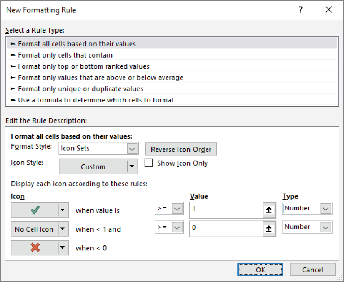
FIGURE 5.15 Changing the icon assignment rule

FIGURE 5.16 Using a modified rule and eliminating an icon makes the table more readable.
The last entry in the New Formatting Rule dialog box is Use a Formula to Determine Which Cells to Format. This is the entry you choose if none of the other shortcuts do what you want. It provides maximum flexibility for creating a rule.
Understanding relative and absolute references
If the formula that you enter into the New Formatting Rule or Edit Formatting Rule dialog box contains a cell reference, that reference is considered a relative reference based on the upper-left cell in the selected range.
For example, suppose that you want to set up a conditional formatting condition that applies shading to cells in range A1:B10 only if the cell contains text. None of Excel's conditional formatting options can do this task, so you need to create a formula that will return TRUE if the cell contains text and FALSE otherwise. Follow these steps:
- Select the range A1:B10, and make sure that cell A1 is the active cell.
- Choose Home ➪ Styles ➪ Conditional Formatting ➪ New Rule. The New Formatting Rule dialog box appears.
- Click the Use a Formula to Determine Which Cells to Format rule type.
- Enter the following formula into the Formula box:
=ISTEXT(A1)
- Click the Format button. The Format Cells dialog box appears.
- From the Fill tab, specify the cell shading that will be applied if the formula returns TRUE.
- Click OK to return to the New Formatting Rule dialog box (see Figure 5.17).
- Click OK to close the New Formatting Rule dialog box.
Notice that the formula entered in step 4 contains a relative reference to the upper-left cell in the selected range.
Generally, when entering a conditional formatting formula for a range of cells, you'll use a reference to the active cell, which is typically the upper-left cell in the selected range. One exception is when you need to refer to a specific cell. For example, suppose that you select range A1:B10 and you want to apply formatting to all cells in the range that exceed the value in cell C1. Enter this conditional formatting formula:
=A1>$C$1
FIGURE 5.17 Creating a conditional formatting rule based on a formula
In this case, the reference to cell C1 is an absolute reference; it will not be adjusted for the cells in the selected range. In other words, the conditional formatting formula for cell A2 looks like this:
=A2>$C$1The relative cell reference is adjusted, but the absolute cell reference is not.
Conditional formatting formula examples
Each of these examples uses a formula entered directly into the New Formatting Rule dialog box after the Use a Formula to Determine Which Cells to Format rule type is selected. You decide the type of formatting that you apply conditionally.
Identifying weekend days
Excel provides a number of conditional formatting rules that deal with dates, but it doesn't let you identify dates that fall on a weekend. Use this formula to identify weekend dates:
=OR(WEEKDAY(A1)=7,WEEKDAY(A1)=1)This formula assumes that a range is selected and that cell A1 is the active cell.
Highlighting a row based on a value
Figure 5.18 shows part of a worksheet that contains a conditional formula in the range A3:G28. If a name entered in cell B1 is found in the first column, the entire row for that name is highlighted.

FIGURE 5.18 Highlighting a row, based on a matching name
The conditional formatting formula is:
=$A3=$B$1Notice that a mixed reference is used for cell A3. Because the column part of the reference is absolute, the comparison is always done using the contents of column A.
Displaying alternate-row shading
The conditional formatting formula that follows was applied to the range A1:D18, as shown in Figure 5.19, to apply shading to alternate rows:
=MOD(ROW(),2)=0 Alternate row shading can make your spreadsheets easier to read. If you add or delete rows within the conditional formatting area, the shading is updated automatically.
This formula uses the ROW function (which returns the row number) and the MOD function (which returns the remainder of its first argument divided by its second argument). For cells in even-numbered rows, the MOD function returns 0, and cells in that row are formatted.
For alternate shading of columns, use the COLUMN function instead of the ROW function.
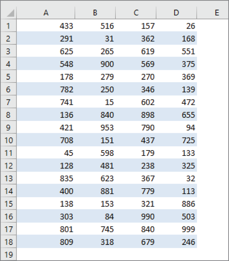
FIGURE 5.19 Using conditional formatting to apply formatting to alternate rows
Creating checkerboard shading
The following formula is a variation on the example in the preceding section. It applies formatting to alternate rows and columns, creating a checkerboard effect.
=MOD(ROW(),2)=MOD(COLUMN(),2)Shading groups of rows
Here's another row shading variation. The following formula shades alternate groups of rows. It produces four shaded rows, followed by four unshaded rows, followed by four more shaded rows, and so on.
=MOD(INT((ROW()-1)/4)+1,2)=1Figure 5.20 shows an example.
For different sized groups, change the 4 to some other value. For example, use this formula to shade alternate groups of two rows:
=MOD(INT((ROW()-1)/2)+1,2)=1Working with conditional formats
The following sections describe some additional information about conditional formatting that you may find useful.

FIGURE 5.20 Conditional formatting produces these groups of alternating shaded rows.
Managing rules
The Conditional Formatting Rules Manager dialog box is useful for checking, editing, deleting, and adding conditional formats. First select any cell in the range that contains conditional formatting. Then choose Home ➪ Styles ➪ Conditional Formatting ➪ Manage Rules.
You can specify as many rules as you like by clicking the New Rule button. Cells can even use data bars, color scales, and icon sets at the same time.
Copying cells that contain conditional formatting
Conditional formatting information is stored with a cell much like standard formatting information is stored with a cell. As a result, when you copy a cell that contains conditional formatting, you also copy the conditional formatting.
If you insert rows or columns within a range that contains conditional formatting, the new cells have the same conditional formatting.
Deleting conditional formatting
When you press Delete to delete the contents of a cell, you don't delete the conditional formatting for the cell (if any). To remove all conditional formats (as well as all other cell formatting), select the cell and then choose Home ➪ Editing ➪ Clear ➪ Clear Formats. Or, choose Home ➪ Editing ➪ Clear ➪ Clear All to delete the cell contents and the conditional formatting.
To remove only conditional formatting (and leave the other formatting intact), choose Home ➪ Styles ➪ Conditional Formatting ➪ Clear Rules and choose one of the available options.
Locating cells that contain conditional formatting
You can't always tell, just by looking at a cell, whether it contains conditional formatting. You can, however, use the Go To Special dialog box to select such cells.
- Choose Home ➪ Editing ➪ Find & Select ➪ Go To Special. The Go To Special dialog box appears.
- In the Go To Special dialog box, select the Conditional Formats option.
- To select all cells on the worksheet containing conditional formatting, select the All option. To select only the cells that contain the same conditional formatting as the active cell, select the Same option.
- Click OK. Excel selects the cells for you.
Using Named Styles for Easier Formatting
One of the most underutilized features in Excel is named styles. Named styles make it easy to apply a set of predefined formatting options to a cell or range. In addition to saving time, using named styles helps to ensure a consistent look.
A style can consist of settings for up to six attributes:
- Number format
- Alignment (vertical and horizontal)
- Font (type, size, and color)
- Borders
- Fill
- Cell protection (locked and hidden)
The real power of styles is apparent when you change a component of a style. All cells that use that named style automatically incorporate the change. Suppose that you apply a particular style to a dozen cells scattered throughout your worksheet. Later, you realize that these cells should have a font size of 14 pt rather than 12 pt. Rather than change each cell, simply edit the style. All cells with that particular style change automatically.
Applying styles
Excel includes a good selection of predefined named styles that work in conjunction with document themes. Figure 5.21 shows the effect of choosing Home ➪ Styles ➪ Cell Styles. Note that this display is a live preview—as you move your mouse over the style choices, the selected cell or range temporarily displays the style. When you see a style you like, click it to apply the style to the selection.
After you apply a style to a cell, you can apply additional formatting to it by using any formatting method discussed in this chapter. Formatting modifications that you make to the cell don't affect other cells that use the same style.
You have quite a bit of control over styles. In fact, you can do any of the following:
- Modify an existing style.
- Create a new style.
- Merge styles from another workbook into the active workbook.
The following sections describe these procedures.
Modifying an existing style
To change an existing style, choose Home ➪ Styles ➪ Cell Styles. Right-click the style that you want to modify and choose Modify from the shortcut menu. Excel displays the Style dialog box, as shown in Figure 5.22. In this example, the Style dialog box shows the settings for the Office theme Normal style—which is the default style for all cells. The style definitions vary, depending on which document theme is active.

FIGURE 5.21 Excel displays samples of predefined cell styles.
Here's a quick example of how you can use styles to change the default font used throughout your workbook:
- Choose Home ➪ Styles ➪ Cell Styles. Excel displays the list of styles for the active workbook.
- Right-click Normal and choose Modify. Excel displays the Style dialog box (refer to Figure 5.22), with the current settings for the Normal style.
- Click the Format button. Excel displays the Format Cells dialog box.
- Click the Font tab and choose the font and size that you want as the default.
- Click OK to return to the Style dialog box. Notice that the Font item displays the font choice you made.
- Click OK again to close the Style dialog box.
The font for all cells that use the Normal style changes to the font that you specified. You can change any formatting attributes for any style.
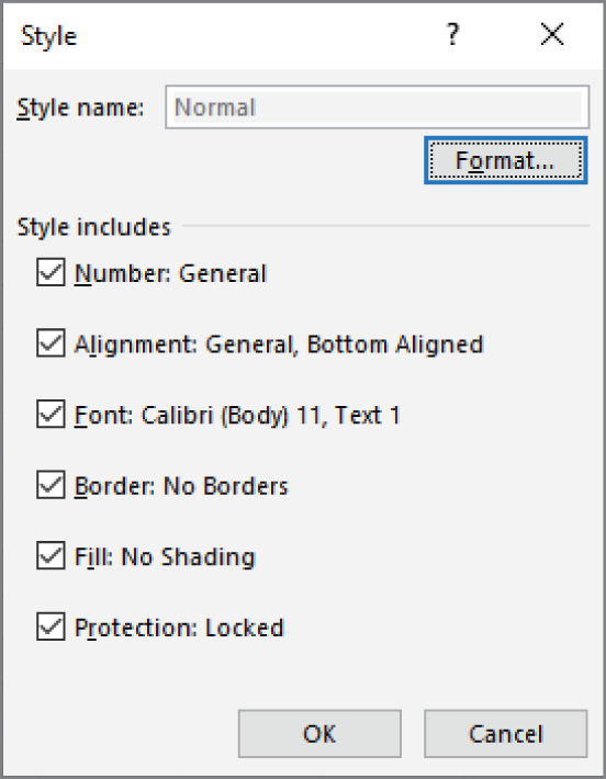
FIGURE 5.22 Use the Style dialog box to modify named styles.
Creating new styles
In addition to using Excel's built-in styles, you can create your own styles. This feature can be quite handy because it enables you to apply your favorite formatting options quickly and consistently.
To create a new style, follow these steps:
- Select a cell and apply all the formatting that you want to include in the new style. You can use any of the formatting that is available in the Format Cells dialog box.
- After you format the cell to your liking, choose Home ➪ Styles ➪ Cell Styles, and choose New Cell Style. Excel displays its Style dialog box (refer to Figure 5.22), along with a proposed generic name for the style. Note that Excel displays the words By Example to indicate that it's basing the style on the current cell.
- Enter a new style name in the Style Name field. The check boxes display the current formats for the cell. By default, all check boxes are selected.
- (Optional) If you don't want the style to include one or more format categories, remove the check(s) from the appropriate check box(es).
- Click OK to create the style and to close the dialog box.
After you perform these steps, the new custom style is available when you choose Home ➪ Styles ➪ Cell Styles. To delete a custom style, right-click it in the Styles gallery and choose Delete. Custom styles are available only in the workbook in which they were created. To copy your custom styles to another workbook, see the section that follows.
Merging styles from other workbooks
Custom styles are stored with the workbook in which they were created. If you've created some custom styles, you probably don't want to go through all of the work required to create copies of those styles in each new Excel workbook. A better approach is to merge the styles from a workbook in which you previously created them.
To merge styles from another workbook, open both the workbook that contains the styles that you want to merge and the workbook that will contain the merged styles. Activate the second workbook, choose Home ➪ Styles ➪ Cell Styles, and then choose Merge Styles. Excel displays the Merge Styles dialog box that shows a list of all open workbooks. Select the workbook that contains the styles you want to merge and click OK. Excel copies custom styles from the workbook that you selected into the active workbook.
Controlling styles with templates
When you start Excel, it loads with several default settings, including the settings for stylistic formatting. If you spend a lot of time changing the default elements for every new workbook, you should know about templates.
Here's an example. You may prefer that gridlines aren't displayed in worksheets. And maybe you prefer Wrap Text to be the default setting for alignment. Templates provide an easy way to change defaults.
The trick is to create a workbook with the Normal style modified in the way you want it. Then save the workbook as a template (with an .xltx extension). After doing so, you can choose this template as the basis for a new workbook.
Understanding Document Themes
In an attempt to help users create more professional-looking documents, the Office designers incorporated a feature known as document themes. Using themes is an easy (and almost foolproof) way to specify colors, fonts, and a variety of graphic effects in a document. Best of all, changing the entire look of your document is a breeze. A few mouse clicks is all that it takes to apply a different theme and change the look of your workbook.
Importantly, the concept of themes is incorporated into other Office applications. Therefore, a company can easily create a standard and consistent look for all of its documents.
Figure 5.23 shows a worksheet that contains a SmartArt diagram, a table, a chart, and a range formatted with the Title named style, and a range formatted with the Explanatory Text named style. These items all use the default theme, which is the Office theme.

FIGURE 5.23 The elements in this worksheet use the default theme.
Figure 5.24 shows the same worksheet after applying a different document theme. The different theme changed the fonts, the colors (which may not be apparent in the figure), and the graphics effects for the SmartArt diagram.

FIGURE 5.24 The worksheet after applying a different theme
Applying a theme
Figure 5.25 shows the theme choices that appear when you choose Page Layout ➪ Themes ➪ Themes. This display is a live preview. As you move your mouse over the theme choices, the active worksheet displays the theme. When you see a theme you like, click it to apply the theme to all worksheets in the workbook.

FIGURE 5.25 Built-in Excel theme choices
When you specify a particular theme, the gallery choices for various elements reflect the new theme. For example, the chart styles that you can choose from vary, depending on which theme is active.
Customizing a theme
Notice that the Themes group on the Page Layout tab contains three other controls: Colors, Fonts, and Effects. You can use these controls to change just one of the three components of a theme. For example, you might like the colors and effects in the Office theme but would prefer different fonts. To change the font set, apply the Office theme and then specify your preferred font set by choosing Page Layout ➪ Themes ➪ Fonts.
Each theme uses two fonts (one for headers and one for the body), and in some cases these two fonts are the same. If none of the theme choices is suitable, choose Page Layout ➪ Themes ➪ Fonts ➪ Customize Fonts to specify the two fonts that you prefer (see Figure 5.26).

FIGURE 5.26 Use this dialog box to specify two fonts for a theme.
Choose Page Layout ➪ Themes ➪ Colors to select a different set of colors. And, if you're so inclined, you can even create a custom set of colors by choosing Page Layout ➪ Themes ➪ Colors ➪ Customize Colors. This command displays the Create New Theme Colors dialog box, as shown in Figure 5.27. Note that each theme consists of twelve colors. Four of the colors are for text and backgrounds, six are for accents, and two are for hyperlinks. As you specify different colors, the preview panel in the dialog box updates.
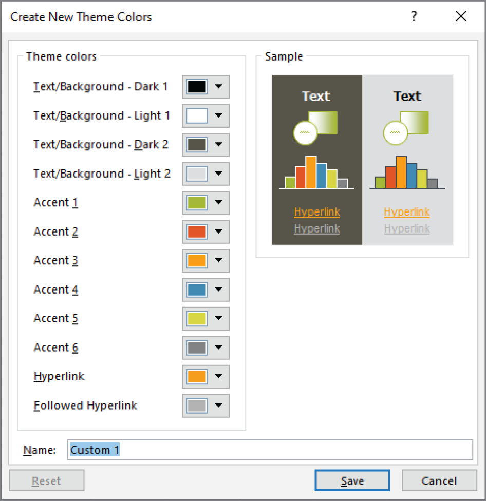
FIGURE 5.27 If you're feeling creative, you can specify a set of custom colors for a theme.
If you've customized a theme using different fonts or colors, you can save the new theme by choosing Page Layout ➪ Themes ➪ Save Current Theme. Your customized themes appear in the Themes list in the Custom category. Other Office applications, such as Word and PowerPoint, can use these theme files. If you need to delete your custom theme, right-click it in the Themes gallery and choose Delete.