
CHAPTER 3
Performing Basic Worksheet Operations
This chapter covers some basic information regarding workbooks, worksheets, and windows. You'll discover tips and techniques to help you take control of your worksheets and help you to work more efficiently.
Learning the Fundamentals of Excel Worksheets
In Excel, each file is called a workbook, and each workbook can contain one or more worksheets. You may find it helpful to think of an Excel workbook as a binder and worksheets as pages in the binder. As with a binder, you can view a particular sheet, add new sheets, remove sheets, rearrange sheets, and copy sheets.
A workbook can hold any number of sheets, and these sheets can be either worksheets (sheets consisting of rows and columns) or chart sheets (sheets that hold a single chart). A worksheet is what people usually think of when they think of a spreadsheet.
The following sections describe the operations that you can perform with windows and worksheets.
Working with Excel windows
Each Excel workbook file that you open is displayed in a window. A window is the operating system's container for that workbook. You can open as many Excel workbooks as necessary at the same time.
Each Excel window has five icons at the right side of its title bar. From left to right, they are Account, Ribbon Display Options, Minimize, Maximize (or Restore Down), and Close.
An Excel window can be in one of the following states:
- Maximized Fills the entire screen. To maximize a window, click its Maximize button.
- Minimized Hidden but still open. To minimize a window, clicks its Minimize button.
- Restored Visible but smaller than the whole screen. To restore a maximized window, click its Restore Down button. To restore a minimized window, click its icon in the Windows taskbar. A window in this state can be resized and moved.
If you work with more than one workbook simultaneously (which is quite common), you need to know how to move, resize, close, and switch among the workbook windows.
Moving and resizing windows
To move a window, click and drag its title bar with your mouse. If it's maximized, it will change to a restored state. If it's already in a restored state, it will maintain its current size.
To resize a window, click and drag any of its borders until it's the size that you want it to be. When you position the mouse pointer on a window's border, the mouse pointer changes to a double arrow, which lets you know that you can now click and drag to resize the window. To resize a window horizontally and vertically at the same time, click and drag any of its corners.
If you want all your workbook windows to be visible (that is, not obscured by another window), you can move and resize the windows manually, or you can let Excel do it for you. Choosing View ➪ Window ➪ Arrange All displays the Arrange Windows dialog box, as shown in Figure 3.1. This dialog box has four window arrangement options. Just select the one that you want and click OK. Windows that are minimized aren't affected by this command.
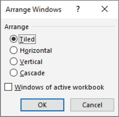
FIGURE 3.1 Use the Arrange Windows dialog box to arrange all open non-minimized workbook windows quickly.
Switching among windows
At any given time, one (and only one) workbook window is the active window. The active window accepts your input, and it is the window on which your commands work. The text in the active window's title bar is brighter than that of other windows. To work in a workbook in a different window, you need to make that window active. You can make a different window the active window in several ways.
- Click another window if it's visible. The window you click moves to the top and becomes the active window. This method isn't possible if the current window is maximized unless the other window is on a different monitor.
- Press Ctrl+Tab to cycle through all open windows until the window that you want to work with appears on top as the active window. Pressing Ctrl+Shift+Tab cycles through the windows in the opposite direction.
- Press Alt+Tab or Alt+Shift+Tab to cycle through all open windows of all running programs. Since more recent versions of Excel display each Excel window in its own Windows window, you can use this shortcut key combination to switch between them as you would switch between two programs, like between Excel and Word.
- Choose View ➪ Window ➪ Switch Windows and select the window that you want from the drop-down list (the active window has a check mark next to it). This menu can display as many as nine windows. If you have more than nine workbook windows open, choose More Windows (which appears below the nine window names).
- Click the corresponding Excel icon in the Windows taskbar.
You might be one of the many people who prefer to do most work with maximized workbook windows, which enables you to see more cells and eliminates the distraction of other workbook windows getting in the way. At times, however, viewing multiple windows is preferred. For example, displaying two windows is more efficient if you need to compare information in two workbooks or if you need to copy data from one workbook to another.
Closing windows
If you have multiple windows open, you may want to close those windows that you no longer need. Excel offers several ways to close the active window.
- Choose File ➪ Close.
- Click the Close button (the X icon) on the right side of the workbook window's title bar.
- Press Alt+F4.
- Press Ctrl+W.
When you close a workbook window, Excel checks whether you have made any changes since the last time you saved the file. If you have made changes, Excel prompts you to save the file before it closes the window. If you haven't, the window closes without a prompt from Excel.
Sometimes you will be prompted to save a workbook even if you've made no changes to it. This occurs if your workbook contains any volatile functions. Volatile functions recalculate every time the workbook recalculates. For example, if a cell contains =NOW(), you will be prompted to save the workbook because the NOW function updated the cell with the current date and time.
Activating a worksheet
At any given time, one workbook is the active workbook and one sheet is the active sheet in the active workbook. To activate a different sheet, just click its sheet tab, which is located at the bottom of the workbook window. You also can use the following shortcut keys to activate a different sheet:
- Ctrl+PgUp activates the previous sheet if one exists.
- Ctrl+PgDn activates the next sheet if one exists.
If your workbook has many sheets, all its tabs may not be visible. Use the sheet tab controls (see Figure 3.2) to scroll the sheet tabs. Clicking the sheet tab controls scrolls one tab at a time, and Ctrl+clicking scrolls to the first or last sheet. The sheet tabs share space with the worksheet's horizontal scrollbar. You also can drag the tab split control (to the left of the horizontal scrollbar) to display more or fewer tabs. Dragging the tab split control simultaneously changes the number of visible tabs and the size of the horizontal scrollbar.
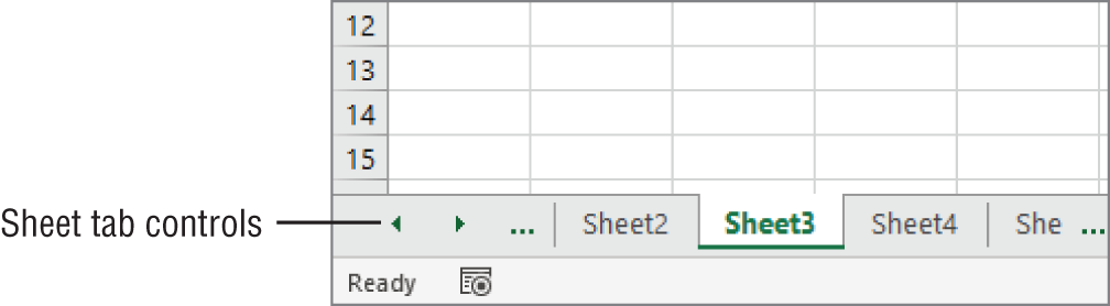
FIGURE 3.2 Use the sheet tab controls to activate a different worksheet or to see additional worksheet tabs.
Adding a new worksheet to your workbook
Worksheets can be an excellent organizational tool. Instead of placing everything on a single worksheet, you can use additional worksheets in a workbook to separate various workbook elements logically. For example, if you have several products whose sales you track individually, you may want to assign each product to its own worksheet and then use another worksheet to consolidate your results.
Here are four ways to add a new worksheet to a workbook:
- Click the New sheet button, which is the plus sign icon located to the right of the last visible sheet tab. A new sheet is added after the active sheet.
- Press Shift+F11. A new sheet is added before the active sheet.
- From the Ribbon, choose Home ➪ Cells ➪ Insert ➪ Insert Sheet. A new sheet is added before the active sheet.
- Right-click a sheet tab, choose Insert from the shortcut menu, and select the General tab of the Insert dialog box that appears. Then select the Worksheet icon and click OK. A new sheet is added before the active sheet.
Deleting a worksheet you no longer need
If you no longer need a worksheet or if you want to get rid of an empty worksheet in a workbook, you can delete it in either of two ways.
- Right-click its sheet tab and choose Delete from the shortcut menu.
- Activate the unwanted worksheet and choose Home ➪ Cells ➪ Delete ➪ Delete Sheet.
If the worksheet is not empty, Excel asks you to confirm that you want to delete the sheet (see Figure 3.3).
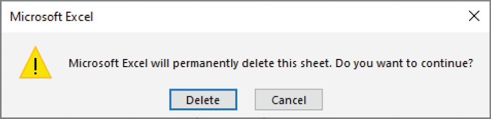
FIGURE 3.3 Excel's warning that you might be losing some data
Changing the name of a worksheet
The default names that Excel uses for worksheets—Sheet1, Sheet2, and so on—are generic and nondescriptive. To make it easier to locate data in a multisheet workbook, you'll want to make the sheet names more descriptive.
These are three ways to change a sheet's name:
- From the Ribbon, choose Home ➪ Cells ➪ Format ➪ Rename Sheet.
- Double-click the sheet tab.
- Right-click the sheet tab and choose Rename.
Excel highlights the name on the sheet tab so that you can edit the name or replace it with a new name. While you're editing a sheet name, all the normal text selection techniques work, such as Home, End, arrow keys, and Shift+arrow keys. Press Enter when you're finished editing and the focus will be back on the active cell.
Sheet names can contain as many as 31 characters, and spaces are allowed. However, you can't use the following characters in sheet names:
| : | Colon |
| / | Slash |
| Backslash | |
| [ ] | Square brackets |
| ? | Question mark |
| * | Asterisk |
Keep in mind that a longer worksheet name results in a wider tab, which takes up more space onscreen. Therefore, if you use lengthy sheet names, you won't be able to see as many sheet tabs without scrolling the tab list.
Changing a sheet tab color
Excel allows you to change the background color of your worksheet tabs. For example, you may prefer to color-code the sheet tabs to make identifying the worksheet's contents easier.
To change the color of a sheet tab, choose Home ➪ Cells ➪ Format ➪ Tab Color, or right-click the tab and choose Tab Color from the shortcut menu. Then select the color from the color palette. You can't change the text color, but Excel will choose a contrasting color to make the text visible. For example, if you make a sheet tab black, Excel will display white text.
If you change a sheet tab's color, the tab shows a gradient from that color to white when the sheet is active. When a different sheet is active, the whole tab appears in the selected color.
Rearranging your worksheets
You may want to rearrange the order of worksheets in a workbook. If you have a separate worksheet for each sales region, for example, arranging the worksheets in alphabetical order might be helpful. You can also move a worksheet from one workbook to another and create copies of worksheets, either in the same workbook or in a different workbook.
You can move a worksheet in the following ways:
- Right-click the sheet tab and choose Move or Copy to display the Move or Copy dialog box (see Figure 3.4). Use this dialog box to specify the location for the sheet.
- From the Ribbon, choose Home ➪ Cells ➪ Format ➪ Move or Copy Sheet. This shows the same dialog box as the previous method.
- Click the worksheet tab and drag it to its desired location. When you drag, the mouse pointer changes to a small sheet icon, and a small arrow indicates where the sheet will be placed when you release the mouse button. To move a worksheet to a different workbook by dragging, both workbooks must be visible.
Copying the worksheet is similar to moving it. If you use one of the options that shows the Move or Copy dialog box, select the Create a Copy check box. To drag and create a copy, hold down the Ctrl key while you drag the worksheet tab. The mouse pointer will change to a small sheet icon with a plus sign on it.
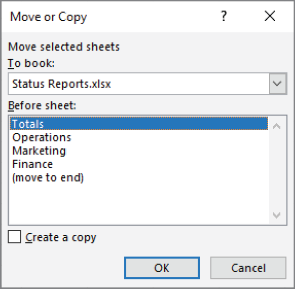
FIGURE 3.4 Use the Move or Copy dialog box to move or copy worksheets in the same or another workbook.
If you move or copy a worksheet to a workbook that already has a sheet with the same name, Excel changes the name to make it unique. For example, Sheet1 becomes Sheet1 (2). You probably want to rename the copied sheet to give it a more meaningful name. (See “Changing the name of a worksheet” earlier in this chapter.)
Hiding and unhiding a worksheet
In some situations, you may want to hide one or more worksheets. Hiding a sheet may be useful if you don't want others to see it or if you just want to get it out of the way. When a sheet is hidden, its sheet tab is also hidden. You can't hide all the sheets in a workbook; at least one sheet must remain visible.
To hide a worksheet, choose Home ➪ Cells ➪ Format ➪ Hide & Unhide ➪ Hide Sheet, or right-click its sheet tab and choose Hide. The active worksheet (or selected worksheets) will be hidden from view.
To unhide a hidden worksheet, choose Home ➪ Cells ➪ Format ➪ Hide & Unhide ➪ Unhide Sheet, or right-click any sheet tab and choose Unhide. Excel opens the Unhide dialog box, which lists all hidden sheets. Choose the sheet that you want to redisplay and click OK. You can select multiple sheets from this dialog box by holding down the Ctrl key and clicking the sheets to unhide. Hold down the Shift key and click a sheet to select a range of contiguous sheets. When you unhide a sheet, it appears in its previous position among the sheet tabs.
Controlling the Worksheet View
As you add more information to a worksheet, you may find that navigating and locating what you want becomes more difficult. Excel includes a few options that enable you to view your sheet, and sometimes multiple sheets, more efficiently. The following sections discuss a few additional worksheet options at your disposal.
Zooming in or out for a better view
Normally, everything you see onscreen is displayed at 100%. You can change the zoom percentage from 10% (very tiny) to 400% (huge). Zooming out by using a small zoom percentage can help you get a bird's-eye view of your worksheet to see how it's laid out. Zooming in by using a large zoom percentage is useful if you have trouble deciphering tiny type. Zooming doesn't change the font size specified for the cells, so it has no effect on printed output.
You can change the zoom factor of the active worksheet window by using any of these three methods:
- Use the Zoom slider located on the right side of the status bar. Click and drag the slider, and your screen transforms as you slide. You can also click anywhere on the Zoom slider to move the bar directly to that spot or use the Zoom In (+) or Zoom Out (-) buttons on either side of the slider to change the zoom by 10%.
- Press Ctrl and use the wheel button on your mouse to zoom in or out.
- Choose View ➪ Zoom ➪ Zoom, which displays a dialog box with some zoom options.
Also in the Zoom Ribbon group is a 100% button to return to 100% zoom quickly and a Zoom to Selection button to change the zoom so that whatever cells you have selected take up the whole window (but still limited to the 10%–400% zoom range).
Viewing a worksheet in multiple windows
Sometimes, you may want to view two different parts of a worksheet simultaneously—perhaps to make referencing a distant cell in a formula easier. Or you may want to examine more than one sheet in the same workbook simultaneously. You can accomplish either of these actions by opening a new view to the workbook, using one or more additional windows.
To create and display a new view of the active workbook, choose View ➪ Window ➪ New Window.
Excel displays a new window for the active workbook, similar to the one shown in Figure 3.5. In this case, each window shows a different worksheet in the workbook. Notice the text in the active window's title bar is FinancialInformation.xlsm - 2. To help you keep track of the windows, Excel appends a hyphen and a number to each window.
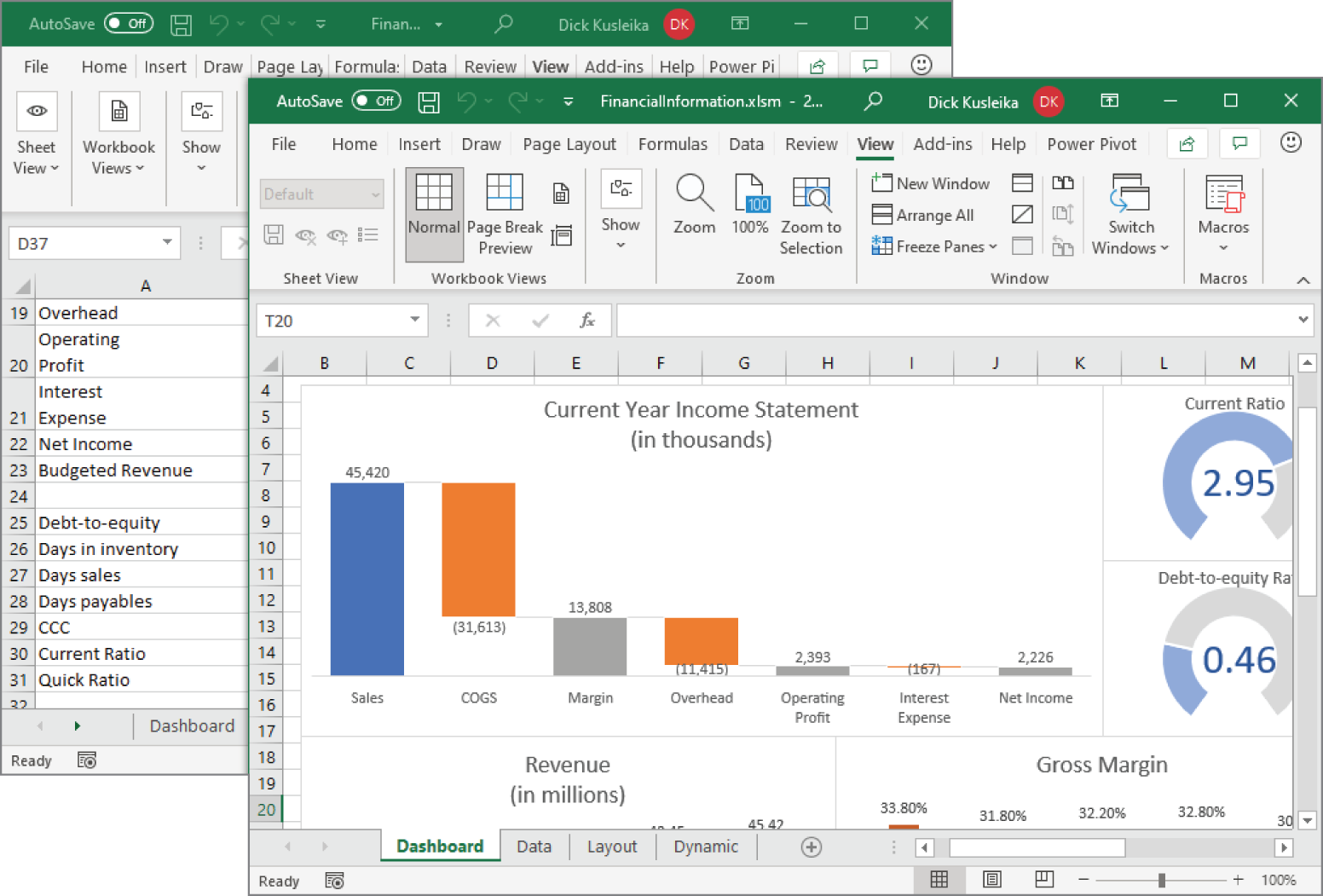
FIGURE 3.5 Use multiple windows to view different sections of a workbook at the same time.
A single workbook can have as many views (that is, separate windows) as you want. Each window is independent. In other words, scrolling to a new location in one window doesn't cause scrolling in the other window(s). However, if you make changes to the worksheet shown in a particular window, those changes are also made in all views of that worksheet.
You can close these additional windows when you no longer need them. For example, clicking the Close button on the active window's title bar closes the active window but doesn't close the other windows for the workbook. If you have unsaved changes, Excel will prompt you to save only when you close the last window.
Comparing sheets side by side
In some situations, you may want to compare two worksheets that are in different windows. The View Side by Side feature makes this task a bit easier.
First, make sure that the two sheets are displayed in separate windows. (The sheets can be in the same workbook or in different workbooks.) If you want to compare two sheets in the same workbook, choose View ➪ Window ➪ New Window to create a new window for the active workbook. Activate the first window; then choose View ➪ Window ➪ View Side by Side. If more than two windows are open, you see a dialog box that lets you select the window for the comparison. The two windows are tiled to fill the entire screen.
When using the Compare Side by Side feature, scrolling in one of the windows also scrolls the other window. If you don't want this simultaneous scrolling, choose View ➪ Window ➪ Synchronous Scrolling (which is a toggle). If you have rearranged or moved the windows, choose View ➪ Window ➪ Reset Window Position to restore the windows to the initial side-by-side arrangement. To turn off the side-by-side viewing, choose View ➪ Window ➪ View Side by Side again.
Keep in mind that this feature is for manual comparison only. Unfortunately, Excel doesn't provide a way to identify the differences between two sheets automatically.
Splitting the worksheet window into panes
If you prefer not to clutter your screen with additional windows, Excel provides another option for viewing multiple parts of the same worksheet. Choosing View ➪ Window ➪ Split splits the active worksheet into two or four separate panes. The split occurs at the location of the active cell. If the active cell is in row 1 or column A, this command results in a two-pane split; otherwise, it gives you four panes. You can use the mouse to drag the split separating individual panes to resize them.
Figure 3.6 shows a worksheet split into four panes. Notice that row numbers aren't continuous. The top panes show rows 7 through 9, and the bottom panes show rows 40 through 57. In other words, splitting panes enables you to display widely separated areas of a worksheet in a single window. To remove the split panes, choose View ➪ Window ➪ Split again or double-click the split bar(s).
Keeping the titles in view by freezing panes
If you set up a worksheet with column headings or descriptive text in the first column, this identifying information won't be visible when you scroll down or to the right. Excel provides a handy solution to this problem: freezing panes. Freezing panes keeps the column or row headings visible while you're scrolling through the worksheet.
To freeze panes, start by moving the active cell to the cell below the row(s) that you want to remain visible while you scroll vertically and to the right of the column(s) that you want to remain visible while you scroll horizontally. Then choose View ➪ Window ➪ Freeze Panes and select the Freeze Panes option from the drop-down list. Excel inserts dark lines to indicate the frozen rows and columns. The frozen rows and columns remain visible while you scroll throughout the worksheet. To remove the frozen panes, choose View ➪ Window ➪ Freeze Panes, and select the Unfreeze Panes option from the drop-down list.
Figure 3.7 shows a worksheet with frozen panes. In this case, row 1 and column A are frozen in place. (Cell B2 was the active cell when the View ➪ Window ➪ Freeze Panes ➪ Freeze Panes command was used.) This technique allows you to scroll down and to the right to locate some information while keeping the column titles and the column A entries visible.
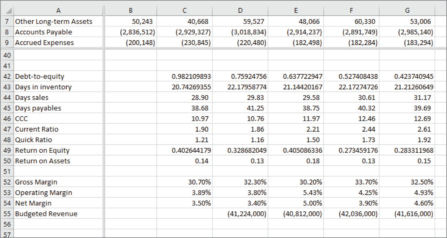
FIGURE 3.6 You can split the worksheet window into two or four panes to view different areas of the worksheet at the same time.
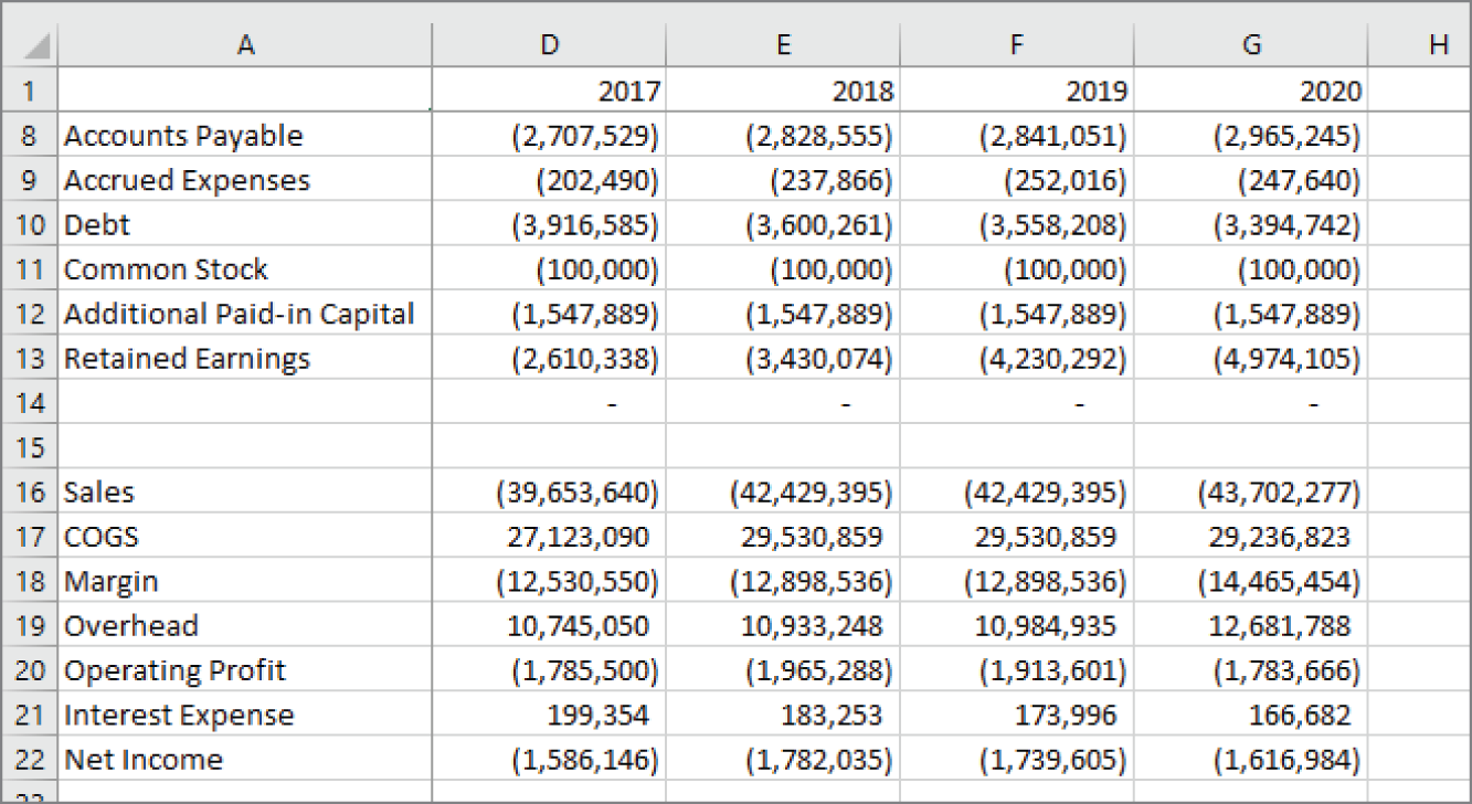
FIGURE 3.7 Freeze certain columns and rows to make them remain visible while you scroll the worksheet.
Most of the time you'll want to freeze either the first row or the first column. The View ➪ Window ➪ Freeze Panes drop-down list has two additional options: Freeze Top Row and Freeze First Column. Using these commands eliminates the need to position the active cell before freezing panes.
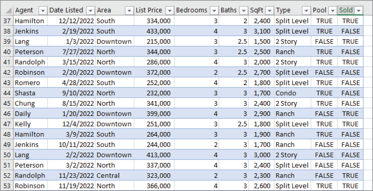
FIGURE 3.8 When using a table, scrolling down displays the table headings where the column letters normally appear.
Monitoring cells with a Watch Window
In some situations, you may want to monitor the value in a particular cell as you work. As you scroll throughout the worksheet, that cell may disappear from view. A feature known as a Watch Window can help. A Watch Window displays the value of any number of cells in a handy window that's always visible.
To display the Watch Window, choose Formulas ➪ Formula Auditing ➪ Watch Window. The Watch Window is actually a task pane, and you can dock it to the side of the window or drag it and make it float over the worksheet.
To add a cell to watch, click Add Watch and specify the cell that you want to watch. The Watch Window displays the value in that cell. You can add any number of cells to the Watch Window. Figure 3.9 shows the Watch Window monitoring cells in different worksheets.
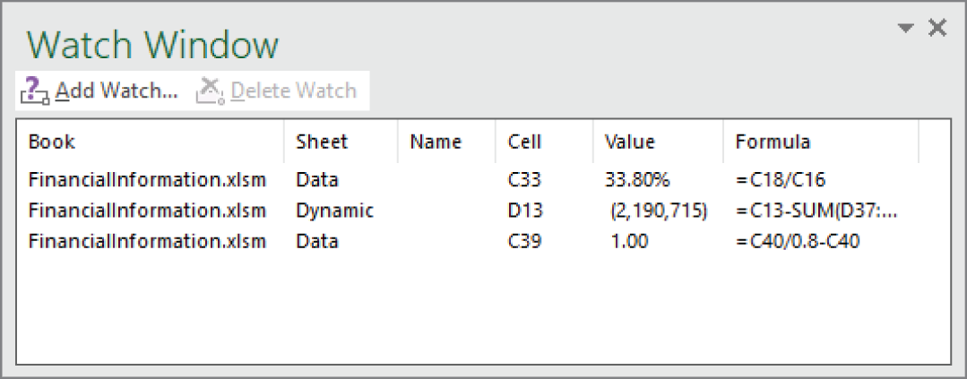
FIGURE 3.9 Use the Watch Window to monitor the value in one or more cells.
Working with Rows and Columns
The following sections discuss worksheet operations that involve complete rows and columns (rather than individual cells). Every worksheet has exactly 1,048,576 rows and 16,384 columns, and these values can't be changed.
Selecting rows and columns
Select an entire row by clicking on the row header or using the Shift+spacebar keyboard shortcut. Select an entire column by clicking on the column header or using the Ctrl+spacebar keyboard shortcut.
If you need to select multiple, contiguous rows or columns, click on the header and drag to the adjacent row or column to extend the selection. You can also click on a row or column header, hold down the Shift key, and click on another row or column to extend the selection. To select rows or columns that aren't contiguous, hold down the Ctrl key while you click each header.
Inserting rows and columns
Although the number of rows and columns in a worksheet is fixed, you can still insert and delete rows and columns if you need to make room for additional information. These operations don't change the number of rows or columns. Instead, inserting a new row moves down the other rows to accommodate the new row. The last row is simply removed from the worksheet if it's empty. Inserting a new column shifts the columns to the right, and the last column is removed if it's empty.
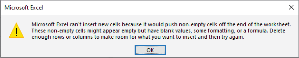
FIGURE 3.10 You can't insert a new row or column if it causes nonblank cells to move off the worksheet.
To insert a new row or rows, use either of these methods:
- Select an entire row or multiple rows by clicking the row numbers in the worksheet border. Right-click and choose Insert from the shortcut menu.
- Select a cell in the row that you want to insert and then choose Home ➪ Cells ➪ Insert ➪ Insert Sheet Rows. If you select multiple cells in the column, Excel inserts additional rows that correspond to the number of cells selected in the column and moves the rows below the insertion down.
To insert a new column or columns, use either of these methods:
- Select an entire column or columns by clicking the column letters in the worksheet border. Right-click and choose Insert from the shortcut menu.
- Select a cell in the column that you want to insert and then choose Home ➪ Cells ➪ Insert ➪ Insert Sheet Columns. If you select multiple cells in the row, Excel inserts additional columns that correspond to the number of cells selected in the row.
You can also insert cells rather than just entire rows or columns. Select the range into which you want to add new cells and then choose Home ➪ Cells ➪ Insert ➪ Insert Cells (or right-click the selection and choose Insert). To insert cells, you must shift the existing cells to the right or down. Therefore, Excel displays the Insert dialog box shown in Figure 3.11 so that you can specify the direction in which you want to shift the cells. Notice that this dialog box also enables you to insert entire rows or columns.
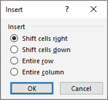
FIGURE 3.11 You can insert partial rows or columns by using the Insert dialog box.
Deleting rows and columns
You may also want to delete rows or columns in a worksheet. For example, your sheet may contain old data that is no longer needed, or you may want to remove empty rows or columns.
To delete a row or rows, use either of these methods:
- Select an entire row or multiple rows by clicking the row numbers in the worksheet border. Right-click and choose Delete from the shortcut menu.
- Move the active cell to the row that you want to delete and then choose Home ➪ Cells ➪ Delete ➪ Delete Sheet Rows. If you select multiple cells in the column, Excel deletes all rows in the selection.
To delete a column or columns, use either of these methods:
- Select an entire column or multiple columns by clicking the column letters in the worksheet border. Right-click and choose Delete from the shortcut menu.
- Move the active cell to the column that you want to delete and then choose Home ➪ Cells ➪ Delete ➪ Delete Sheet Columns. If you select multiple cells in the row, Excel deletes all columns in the selection.
If you discover that you accidentally deleted a row or column, select Undo from the Quick Access Toolbar (or press Ctrl+Z) to undo the action.
Changing column widths and row heights
Often, you'll want to change the width of a column or the height of a row. For example, you can make columns narrower to show more information on a printed page. Or you may want to increase row height to create a “double-spaced” effect.
Excel provides several ways to change the widths of columns and the height of rows.
Changing column widths
Column width is measured in terms of the number of characters of a monospaced font that will fit into the cell's width. By default, each column's width is 8.43 units, which equates to 64 pixels (px).
Before you change the column width, you can select multiple columns so that the width will be the same for all selected columns. To select multiple columns, either click and drag in the column border or press Ctrl while you select individual columns. To select all columns, click the button where the row and column headers intersect. You can change column widths by using any of the following techniques:
- Drag the right-column border with the mouse until the column is the desired width.
- Choose Home ➪ Cells ➪ Format ➪ Column Width and enter a value in the Column Width dialog box.
- Choose Home ➪ Cells ➪ Format ➪ AutoFit Column Width to adjust the width of the selected column so that the widest entry in the column fits. Instead of selecting an entire column, you can just select cells in the column, and the column is adjusted based on the widest entry in your selection.
- Double-click the right border of a column header to set the column width automatically to the widest entry in the column.
Changing row heights
Row height is measured in points (a standard unit of measurement in the printing trade—72 pts is equal to 1 inch). The default row height using the default font is 15 pts, or 20 pixels (px).
The default row height can vary, depending on the font defined in the Normal style. In addition, Excel automatically adjusts row heights to accommodate the tallest font in the row. So, if you change the font size of a cell to 20 pts, for example, Excel makes the row taller so that the entire text is visible.
You can set the row height manually, however, by using any of the following techniques. As with columns, you can select multiple rows:
- Drag the lower row border with the mouse until the row is the desired height.
- Choose Home ➪ Cells ➪ Format ➪ Row Height and enter a value (in points) in the Row Height dialog box.
- Double-click the bottom border of a row to set the row height automatically to the tallest entry in the row. You can also choose Home ➪ Cells ➪ Format ➪ AutoFit Row Height for this task.
Changing the row height is useful for spacing out rows and is almost always preferable to inserting empty rows between lines of data.
Hiding rows and columns
In some cases, you may want to hide rows or columns. Hiding rows and columns may be useful if you don't want users to see particular information or if you need to print a report that summarizes the information in the worksheet without showing all the details.
To hide rows in your worksheet, select the row or rows that you want to hide by clicking in the row header on the left. Then right-click and choose Hide from the shortcut menu. Or you can use the commands on the Home ➪ Cells ➪ Format ➪ Hide & Unhide menu.
To hide columns, select the column or columns that you want to hide. Then right-click and choose Hide from the shortcut menu. Or you can use the commands on the Home ➪ Cells ➪ Format ➪ Hide & Unhide menu.
A hidden row is actually a row with its height set to zero. Similarly, a hidden column has a column width of zero. When you use the navigation keys to move the active cell, cells in hidden rows or columns are skipped. In other words, you can't use the navigation keys to move to a cell in a hidden row or column.
Notice, however, that Excel displays a narrow column heading for hidden columns and a narrow row heading for hidden rows. You can click and drag the column heading to make the column wider—and make it visible again. For a hidden row, click and drag the small row heading to make the row visible.
Another way to unhide a row or column is to choose Home ➪ Editing ➪ Find & Select ➪ Go To (or use one of its two shortcut keys: F5 or Ctrl+G) to select a cell in a hidden row or column. For example, if column A is hidden, you can press F5 and go to cell A1 (or any other cell in column A) to move the active cell to the hidden column. Then you can choose Home ➪ Cells ➪ Format ➪ Hide & Unhide ➪ Unhide Columns.