CHAPTER 2
Entering and Editing Worksheet Data
This chapter describes what you need to know about entering and modifying data in your worksheets. As you'll see, Excel doesn't treat all data equally. Therefore, you need to learn about the various types of data you can use in an Excel worksheet.
Exploring Data Types
An Excel workbook file can hold any number of worksheets, and each worksheet is made up of more than 17 billion cells. A cell can hold any of four basic types of data.
- A numeric value
- Text
- A formula
- An error
A worksheet can also hold charts, diagrams, pictures, buttons, and other objects. These objects aren't contained in cells. Instead, they reside on the worksheet's drawing layer, which is an invisible layer on top of each worksheet.
Numeric values
Numeric values represent a quantity of some type: sales amounts, number of employees, atomic weights, test scores, and so on. Values also can be dates (such as Feb 26, 2022) or times (such as 3:24 AM).
Text entries
Most worksheets also include text in some of the cells. Text can serve as data (for example, a list of employee names), labels for values, headings for columns, or instructions about the worksheet. Text is often used to clarify what the values in a worksheet mean or where the numbers came from.
Text that begins with a number is still considered text. For example, if you type 12 Employees into a cell, Excel considers the entry to be text rather than a numeric value. Consequently, you can't use this cell for numeric calculations. If you need to indicate that the number 12 refers to employees, enter 12 into a cell and then type Employees into the cell to the right.
Formulas
Formulas are what make a spreadsheet a spreadsheet. Excel enables you to enter flexible formulas that use the values (or even text) in cells to calculate a result. When you enter a formula into a cell, the formula's result appears in the cell. If you change any of the cells used by a formula, the formula recalculates and shows the new result.
Formulas can be simple mathematical expressions, or they can use some of the powerful functions that are built into Excel. Figure 2.1 shows an Excel worksheet set up to calculate a monthly loan payment. The worksheet contains values, text, and formulas. The cells in column A contain text. Column B contains four values and two formulas. The formulas are in cells B6 and B10. Column D, for reference, shows the actual contents of the cells in column B.

FIGURE 2.1 You can use values, text, and formulas to create useful Excel worksheets.
Error values
The fourth data type cells can hold is an error value. Error values are the results of formulas that contain an error, like the #VALUE! error that results from trying to do addition on a text entry. Error values are primarily used by Excel's calculation engine so that formulas that use the results of other formulas continue to show an error.
Entering Text and Values into Your Worksheets
If you've ever worked in a Windows application, you'll find that entering data into worksheet cells is simple and intuitive. And while there are differences in how Excel stores and displays the different data types, for the most part it just works.
Entering numbers
To enter a numeric value into a cell, select the appropriate cell, type the value, and then press Enter, Tab, or one of the arrow navigation keys. The value is displayed in the cell and appears in the Formula bar when the cell is selected. You can include decimal points and currency symbols when entering values, along with plus signs, minus signs, percent signs, and commas (to separate thousands). If you precede a value with a minus sign or enclose it in parentheses, Excel considers it to be a negative number.
Entering text
Entering text into a cell is just as easy as entering a value: activate the cell, type the text, and then press Enter or a navigation key. A cell can contain a maximum of about 32,000 characters—more than enough to store a typical chapter in this book. Even though a cell can hold a huge number of characters, you'll find that it's not actually possible to display all of these characters.

FIGURE 2.2 The Formula bar, expanded in height to show more information in the cell
What happens when you enter text that's longer than its column's current width? If the cells to the immediate right are blank, Excel displays the text in its entirety, appearing to spill the entry into adjacent cells. If an adjacent cell isn't blank, Excel displays as much of the text as possible. (The full text is contained in the cell; it's just not displayed.) If you need to display a long text string in a cell that's adjacent to a nonblank cell, you have a few choices:
- Edit your text to make it shorter.
- Increase the width of the column (drag the border in the column letter display).
- Use a smaller font.
- Wrap the text within the cell so that it occupies more than one line. Choose Home ➪ Alignment ➪ Wrap Text to toggle wrapping on and off for the selected cell or range.
Using Enter mode
The left side of Excel's status bar normally displays “Ready,” indicating that Excel is ready for you to enter or edit data in the worksheet. If you start typing numbers or text in a cell, the status bar changes to display “Enter” to indicate you're in Enter mode. The most common modes for Excel to be in are Ready, Enter, and Edit. See “Modifying Cell Contents” later in this chapter for more information about Edit mode.
In Enter mode, you are actively entering something into a cell. As you type, the text shows in the cell and in the Formula bar. You haven't actually changed the contents of the cell until you leave Enter mode, which commits the value to the cell. To leave Enter mode, you can press Enter, Tab, or just about any navigation key on your keyboard (like PgUp or Home). The value you typed is committed to the cell, and the status bar changes back to say “Ready.”
You can also leave Enter mode by pressing the Esc key. Pressing Esc ignores your changes and returns the cell to its previous value.
Entering Dates and Times into Your Worksheets
Excel treats dates and times as special types of numeric values. Dates and times are values that are formatted so that they appear as dates or times. If you work with dates and times, you need to understand Excel's date and time system.
Entering date values
Excel handles dates by using a serial number system. The earliest date that Excel understands is January 1, 1900. This date has a serial number of 1. January 2, 1900, has a serial number of 2, and so on. This system makes it easy to deal with dates in formulas. For example, you can enter a formula to calculate the number of days between two dates.
Most of the time, you don't have to be concerned with Excel's serial number date system. You can simply enter a date in a common date format, and Excel takes care of the details behind the scenes. For example, if you need to enter June 1, 2022, you can enter the date by typing June 1, 2022 (or use any of several different date formats). Excel interprets your entry and stores the value 44713, which is the serial number for that date.
Entering time values
When you work with times, you extend Excel's date serial number system to include decimals. In other words, Excel works with times by using fractional days. For example, the date serial number for June 1, 2022, is 44713. Noon on June 1, 2022 (halfway through the day), is represented internally as 44713.5 because the time fraction is added to the date serial number to get the full date/time serial number.
Again, you normally don't have to be concerned with these serial numbers or fractional serial numbers for times. Just enter the time into a cell in a recognized format. In this case, type June 1, 2022 12:00.
Modifying Cell Contents
After you enter a value or text into a cell, you can modify it in several ways.
- Delete the cell's contents.
- Replace the cell's contents with something else.
- Edit the cell's contents.
Deleting the contents of a cell
To delete the contents of a cell, just click the cell and press the Delete key. To delete the contents of more than one cell, select all the cells that you want to delete and then press Delete. Pressing Delete removes the cell's contents but doesn't remove any formatting (such as bold, italic, or the number format) that you may have applied to the cell.
For more control over what gets deleted, you can choose Home ➪ Editing ➪ Clear. This command's drop-down list has six choices.
- Clear All Clears everything from the cell—its contents, formatting, and cell comment (if it has one).
- Clear Formats Clears only the formatting and leaves the value, text, or formula.
- Clear Contents Clears only the cell's contents and leaves the formatting. This has the same effect as pressing Delete.
- Clear Comments and Notes Clears the comment or note (if one exists) attached to the cell.
- Clear Hyperlinks Removes hyperlinks contained in the selected cells. The text and formatting remain, so the cell still looks like it has a hyperlink, but it no longer functions as a hyperlink.
- Remove Hyperlinks Removes hyperlinks in the selected cells, including the cell formatting.
Replacing the contents of a cell
To replace the contents of a cell with something else, just activate the cell, type your new entry, and press Enter or a navigation key. Any formatting applied to the cell remains in place and is applied to the new content.
You can also replace cell contents by dragging and dropping or by copying and pasting data from another cell. In both cases, the cell formatting will be replaced by the format of the new data. To avoid pasting formatting, choose Home ➪ Clipboard ➪ Paste ➪ Values (V), or Home ➪ Clipboard ➪ Paste ➪ Formulas (F).
Editing the contents of a cell
If the cell contains only a few characters, replacing its contents by typing new data usually is easiest. However, if the cell contains lengthy text or a complex formula and you need to make only a slight modification, you probably want to edit the cell rather than re-enter information.
When you want to edit the contents of a cell, you can use one of the following ways to enter Edit mode:
- Double-click the cell to edit the cell contents directly in the cell.
- Select the cell and press F2 to edit the cell contents directly in the cell.
- Select the cell that you want to edit and then click inside the Formula bar to edit the cell contents in the Formula bar.
You can use whichever method you prefer. Some people find editing directly in the cell easier; others prefer to use the Formula bar to edit a cell.
All these methods cause Excel to go into Edit mode. (The word Edit appears at the left side of the status bar at the bottom of the window.) When Excel is in Edit mode, the Formula bar enables two icons: Cancel (the X) and Enter (the check mark). Figure 2.3 shows these two icons. Clicking the Cancel icon cancels editing without changing the cell's contents. (Pressing Esc has the same effect.) Clicking the Enter icon completes the editing and enters the modified contents into the cell. (Pressing Enter has the same effect, except that clicking the Enter icon doesn't change the active cell.)

FIGURE 2.3 When you're editing a cell, the Formula bar enables two new icons: Cancel (X) and Enter (check mark).
When you begin editing a cell, the insertion point appears as a vertical bar, and you can perform the following tasks:
- Add new characters at the location of the insertion point. Move the insertion point by doing one of the following:
- Using the navigation keys to move within the cell
- Pressing Home to move the insertion point to the beginning of the cell
- Pressing End to move the insertion point to the end of the cell
- Select multiple characters. Press Shift while you use the navigation keys.
- Select characters while you're editing a cell. Use the mouse. Just click and drag the mouse pointer over the characters that you want to select.
- Delete a character to the left of the insertion point. The Backspace key deletes the selected text or the character to the left of the insertion point if no characters are selected.
- Delete a character to the right of the insertion point. The Delete key also deletes the selected text. If no text is selected, it deletes the character to the right of the insertion point.
Learning some handy data-entry techniques
You can simplify the process of entering information into your Excel worksheets and make your work go quite a bit faster by using a number of useful tricks, which are described in the following sections.
Automatically moving the selection after entering data
By default, Excel automatically selects the next cell down when you press the Enter key after entering data into a cell. To change this setting, choose File ➪ Options and click the Advanced tab (see Figure 2.4). The check box that controls this behavior is labeled After pressing Enter, move selection. If you enable this option, you can choose the direction in which the selection moves (down, right, up, or left).

FIGURE 2.4 You can use the Advanced tab in the Excel Options dialog box to select several helpful input option settings.
Selecting a range of input cells before entering data
When a range of cells is selected, Excel automatically selects the next cell in the range when you press Enter, even if you disabled the After pressing Enter, move selection option. If the selection consists of multiple rows, Excel moves down the column; when it reaches the end of the selection in the column, it moves to the first selected cell in the next column.
To skip a cell, just press Enter without entering anything. To go backward, press Shift+Enter. If you prefer to enter the data by rows rather than by columns, press Tab rather than Enter. Excel continues to cycle through the selected range until you select a cell outside the range. Any of the navigation keys, like the arrow keys or the Home key, will change the selected range. If you want to navigate within the selected range, you must stick to Enter and Tab.
Using Ctrl+Enter to place information into multiple cells simultaneously
If you need to enter the same data into multiple cells, Excel offers a handy shortcut. Select all the cells that you want to contain the data; enter the value, text, or formula; and then press Ctrl+Enter. The same information is inserted into each cell in the selection.
Changing modes
You can press F2 to change between Enter mode and Edit mode. For example, if you're typing a long sentence in Enter mode and you realize that you spelled a word wrong, you can press F2 to change to Edit mode. In Edit mode, you can move through the sentence with your arrow keys to fix the misspelled word. You can also use the Ctrl+arrow keys to move one word at a time instead of one character at a time. You can continue to enter text in Edit mode or return to Enter mode by pressing F2 again, after which the navigation keys can be used to move to a different cell.
Entering decimal points automatically
If you need to enter lots of numbers with a fixed number of decimal places, Excel has a useful tool that works like some old adding machines. Access the Excel Options dialog box and click the Advanced tab. Select the Automatically Insert a Decimal Point check box and make sure that the Places box is set for the correct number of decimal places for the data you need to enter.
When this option is set, Excel supplies the decimal points for you automatically. For example, if you specify two decimal places, entering 12345 into a cell is interpreted as 123.45. To restore things to normal, just clear the Automatically Insert a Decimal Point check box in the Excel Options dialog box. Changing this setting doesn't affect any values that you already entered.
Using AutoFill to enter a series of values
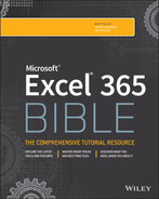
The Excel AutoFill feature makes inserting a series of values or text items in a range of cells easy. It uses the fill handle (the small box at the lower right of the active cell or range). You can drag the fill handle to copy the cell or automatically complete a series.
Figure 2.5 shows an example. Enter 1 into cell A1, and enter 3 into cell A2. Then select both cells and drag down the fill handle to create a linear series of odd numbers. The figure also shows an icon that, when clicked, displays some additional AutoFill options. This icon appears only if the Show Paste Options button when content is pasted option is selected in the Advanced tab of the Excel Options dialog box.
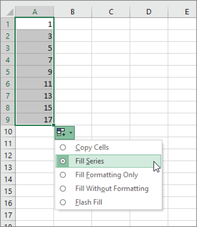
FIGURE 2.5 This series was created by using AutoFill.
Excel uses the cells' data to guess the pattern. If you start with 1 and 2, it will guess you want each cell to go up by 1. If, as in the previous example, you start with 1 and 3, it guesses that you want the increment to be 2. Excel does a good job of guessing date patterns too. If you start with 1/31/2022 and 2/28/2022, it will fill the last day of the successive months.
Using AutoComplete to automate data entry
The Excel AutoComplete feature makes entering the same text into multiple cells easy. With AutoComplete, you type the first few letters of a text entry into a cell, and Excel automatically completes the entry based on other entries that you already made in the column. Besides reducing typing, this feature ensures that your entries are spelled correctly and are consistent.
Here's how it works: Suppose you're entering product information into a column. One of your products is named Widgets. The first time you enter Widgets into a cell, Excel remembers it. Later, when you start typing Widgets in that same column, Excel recognizes it by the first few letters and finishes typing it for you. Just press Enter, and you're done. To override the suggestion, just keep typing.
AutoComplete also changes the case of letters for you automatically. If you start entering widgets (with a lowercase w) in the second entry, Excel makes the w uppercase to be consistent with the previous entry in the column.
Keep in mind that AutoComplete works only within a contiguous column of cells. If you have a blank row, for example, AutoComplete identifies only the cell contents below the blank row.
Sometimes, Excel will use AutoComplete to try to finish a word when you don't want it to do so. If you type canister in a cell and then below it type the shorter word can, Excel will attempt to AutoComplete the entry to canister. When you want to type a word that starts with the same letters as an AutoComplete entry but is shorter, simply press the Delete key when you've reached the end of the word and then press Enter or a navigation key.
If you find the AutoComplete feature distracting, you can turn it off by using the Advanced tab of the Excel Options dialog box. Remove the check mark from the Enable AutoComplete for Cell Values box.
Forcing text to appear on a new line within a cell
If you have lengthy text in a cell, you can force Excel to display it in multiple lines within the cell: press Alt+Enter to start a new line in a cell.
When you add a line break, Excel automatically changes the cell's format to Wrap Text. But unlike normal text wrap, your manual line break forces Excel to break the text at a specific place within the text, which gives you more precise control over the appearance of the text than if you rely on automatic text wrapping.
Using AutoCorrect for shorthand data entry
You can use the AutoCorrect feature to create shortcuts for commonly used words or phrases. For example, if you work for a company named Consolidated Data Processing Corporation, you can create an AutoCorrect entry for an abbreviation, such as cdp. Then, whenever you type cdp and take an action to trigger AutoCorrect (such as typing a space, pressing Enter, or selecting a different cell), Excel automatically changes the text to Consolidated Data Processing Corporation.
Excel includes quite a few built-in AutoCorrect terms (mostly to correct common misspellings), and you can add your own. To set up your custom AutoCorrect entries, access the Excel Options dialog box (choose File ➪ Options) and click the Proofing tab. Then click the AutoCorrect Options button to display the AutoCorrect dialog box. In the dialog box, click the AutoCorrect tab, check the Replace Text as You Type option, and then enter your custom entries. (Figure 2.6 shows an example.) You can set up as many custom entries as you like. Just be careful not to use an abbreviation that might appear normally in your text.
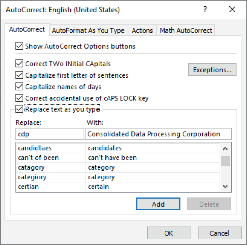
FIGURE 2.6 AutoCorrect allows you to create shorthand abbreviations for text you enter often.
Entering numbers with fractions
Most of the time, you'll want non-integer values to be displayed with decimal points. But Excel can also display values with fractions. To enter a fractional value into a cell, leave a space between the whole number and the fraction. For example, to enter 6 7/8, enter 6 7/8 and then press Enter. When you select the cell, 6.875 appears in the Formula bar, and the cell entry appears as a fraction. If you have a fraction only (for example, 1/8), you must enter a zero first, like this—0 1/8—or Excel will likely assume that you're entering a date. When you select the cell and look at the Formula bar, you see 0.125. In the cell, you see 1/8.
Using a form for data entry
Many people use Excel to manage lists in which the information is arranged in rows. Excel offers a simple way to work with this type of data using a data entry form that Excel can create automatically. This data form works with either a normal range of data or a range that has been designated as a table. (Choose Insert ➪ Tables ➪ Table.) Figure 2.7 shows an example.
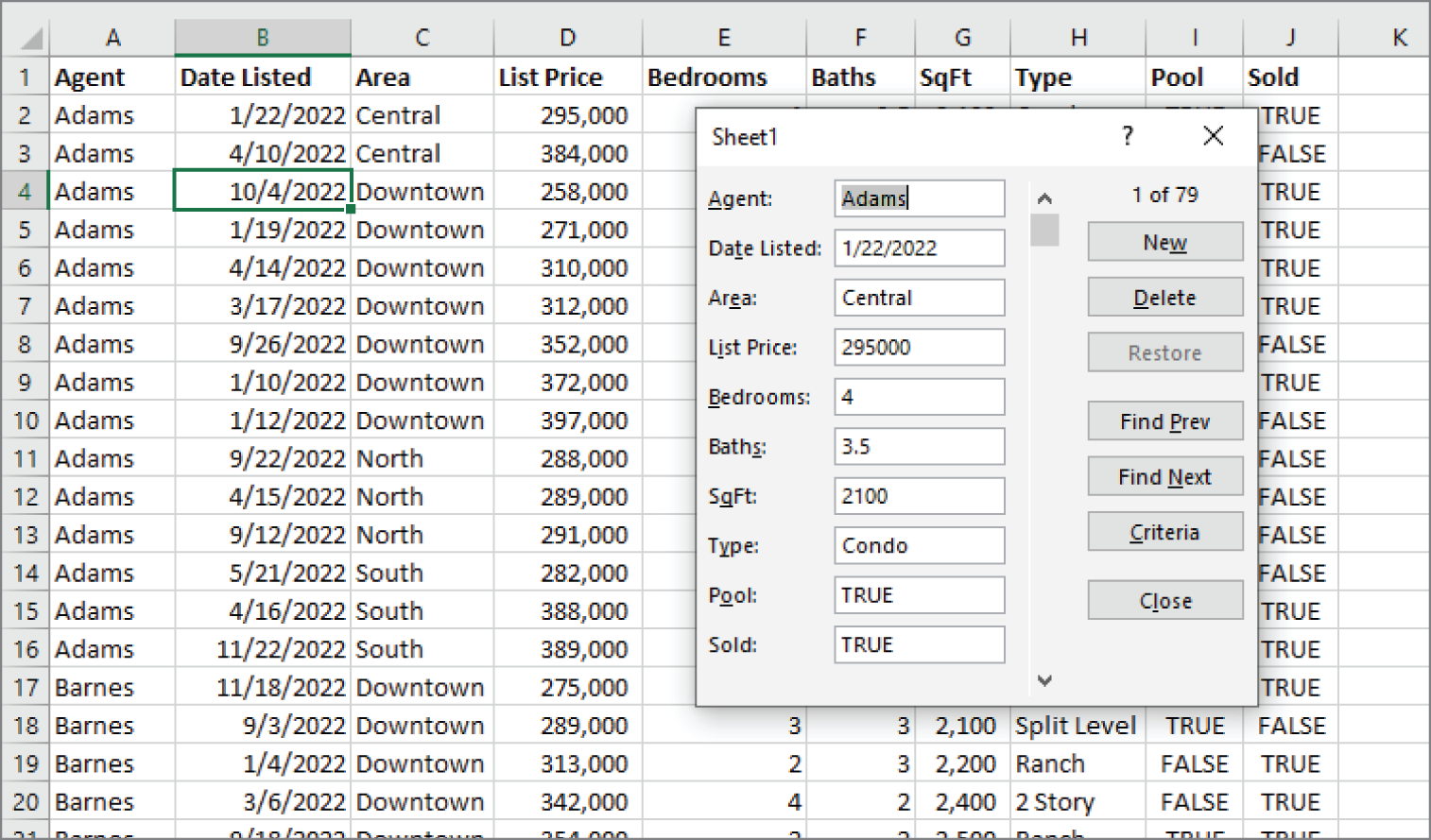
FIGURE 2.7 Excel's built-in data form can simplify many data-entry tasks.
Unfortunately, the command to access the data form is not on the Ribbon. To use the data form, you must add it to your Quick Access Toolbar, add it to the Ribbon, or search for Form in the Search box. Here's how to add this command to your Quick Access Toolbar:
- Right-click the Quick Access Toolbar and choose Customize Quick Access Toolbar. The Quick Access Toolbar panel of the Excel Options dialog box appears.
- In the Choose Commands From drop-down list, choose Commands Not in the Ribbon.
- In the list box on the left, select Form.
- Click the Add button to add the selected command to your Quick Access Toolbar.
- Click OK to close the Excel Options dialog box.
After you perform these steps, a new icon appears on your Quick Access Toolbar.
To use a data entry form, follow these steps:
- Arrange your data so that Excel can recognize it as a table by entering headings for the columns into the first row of your data entry range.
- Select any cell in the table and click the Form button on your Quick Access Toolbar. Excel displays a dialog box customized to your data (refer to the example in Figure 2.7).
- Fill in the information. Press Tab to move between the text boxes. If a cell contains a formula, the formula result appears as text (not as an edit box). In other words, you can't modify formulas using the data entry form.
- When you complete the data form, click the New button. Excel enters the data into a row in the worksheet and clears the dialog box for the next row of data.
You can also use the form to edit existing data.
Entering the current date or time into a cell
If you need to date-stamp or time-stamp your worksheet, Excel provides two shortcut keys that do this task for you:
- Current date: Ctrl+; (semicolon)
- Current time: Ctrl+Shift+; (semicolon)
To enter both the date and time, press Ctrl+;, type a space, and then press Ctrl+Shift+;.
The date and time are from the system time in your computer. If the date or time isn't correct in Excel, use the Windows Settings to make the adjustment.
Applying Number Formatting
Applying number formatting changes the appearance of values contained in cells. Excel provides a variety of number formatting options. In the following sections, you will see how to use many of Excel's formatting options to improve the appearance and readability of your worksheets quickly.
Values that you enter into cells normally are unformatted. In other words, they simply consist of a string of numerals. Typically, you want to format the numbers so that they're easier to read or are more consistent in terms of the number of decimal places shown.
Figure 2.8 shows a worksheet that has two columns of values. The first column consists of unformatted values. The cells in the second column are formatted to make the values easier to read. The third column describes the type of formatting applied.
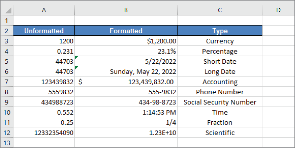
FIGURE 2.8 Use numeric formatting to make it easier to understand what the values in the worksheet represent.
Using automatic number formatting
Excel is able to perform some formatting for you automatically. For example, if you enter 12.2% into a cell, Excel knows that you want to use a percentage format and applies it for you automatically. If you use commas to separate thousands (such as 123,456), Excel applies comma formatting for you. And if you precede your value with a dollar sign, the cell is formatted for currency (assuming that the dollar sign is your system currency symbol).
Anything you enter that can possibly be construed as a date will be treated as such. And depending on how you enter it, Excel will choose a date format to match. If you enter 1/31/2022, Excel will interpret that as a date and format the cell as 1/31/2022 (just as it was entered). If you enter Jan 31, 2022, Excel will format it as 31-Jan-22 (if you omit the comma, Excel won't recognize it as a date). The less obvious example of entering 1-31 causes Excel to display 31-Jan. If you need to enter 1-31 in a cell and it's not supposed to be a date, type an apostrophe (‘) first.
Formatting numbers by using the Ribbon
The Home ➪ Number group on the Ribbon contains controls that let you quickly apply common number formats.
The Number Format drop-down list contains 11 common number formats (see Figure 2.9). Additional options in the Home ➪ Number group include an Accounting Number Format drop-down list (to select a currency format), a Percent Style button, and a Comma Style button. The group also contains a button to increase the number of decimal places and another to decrease the number of decimal places.
When you select one of these controls, the active cell takes on the specified number format. You also can select a range of cells (or even entire rows or columns) before clicking these buttons. If you select more than one cell, Excel applies the number format to all the selected cells.
Using shortcut keys to format numbers
Another way to apply number formatting is to use shortcut keys. Table 2.1 summarizes the shortcut-key combinations that you can use to apply common number formatting to the selected cells or range. Notice that these Ctrl+Shift keys are located together, in the lower left of your keyboard.
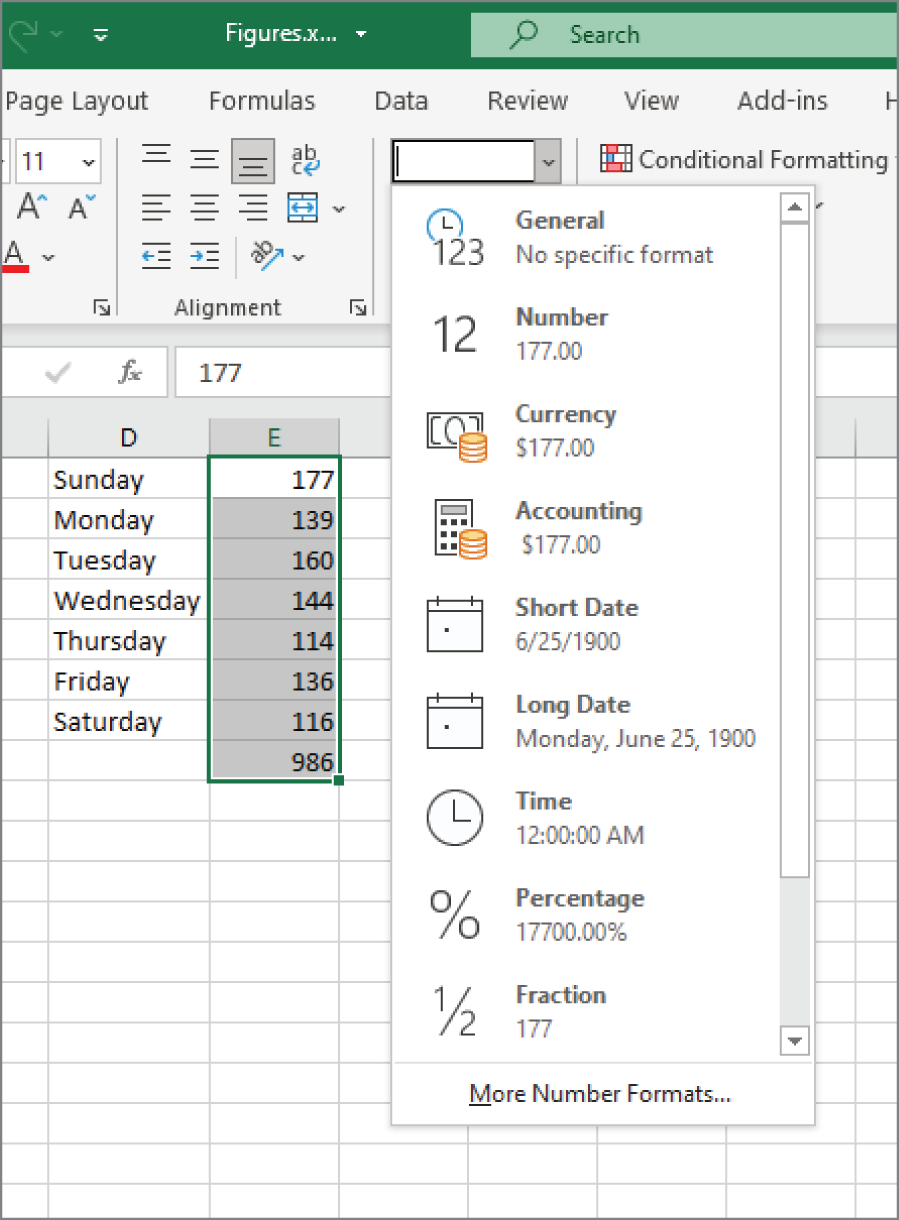
FIGURE 2.9 You can find number formatting commands in the Number group of the Home tab.
TABLE 2.1 Number Formatting Keyboard Shortcuts
| Key Combination | Formatting Applied |
|---|---|
| Ctrl+Shift+~ | General number format (that is, unformatted values) |
| Ctrl+Shift+$ | Currency format with two decimal places (negative numbers appear in red and inside parentheses) |
| Ctrl+Shift+% | Percentage format, with no decimal places |
| Ctrl+Shift+^ | Scientific notation number format, with two decimal places |
| Ctrl+Shift+# | Date format with the day, month, and year |
| Ctrl+Shift+@ | Time format with the hour, minute, and AM or PM |
| Ctrl+Shift+! | Two decimal places, thousands separator, and a hyphen for negative values |
Formatting numbers by using the Format Cells dialog box
In most cases, the number formats that are accessible from the Number group on the Home tab are just fine. Sometimes, however, you want more control over how your values appear. Excel offers a great deal of control over number formats using the Format Cells dialog box, as shown in Figure 2.10. For formatting numbers, you need to use the Number tab.

FIGURE 2.10 When you need more control over number formats, use the Number tab of the Format Cells dialog box.
You can bring up the Format Cells dialog box in several ways. Start by selecting the cell or cells that you want to format and then do one of the following:
- Choose Home ➪ Number and click the small dialog box launcher icon (in the lower-right corner of the Number group).
- Choose Home ➪ Number, click the Number Format drop-down list, and choose More Number Formats from the drop-down list.
- Right-click the cell, and choose Format Cells from the shortcut menu.
- Press Ctrl+1.
The Number tab of the Format Cells dialog box displays 12 categories of number formats. When you select a category from the list box, the right side of the tab changes to display options appropriate to that category.
The Number category has three options that you can control: the number of decimal places displayed, whether to use a thousands separator, and how you want negative numbers displayed. The Negative Numbers list box has four choices (two of which display negative values in red), and the choices change depending on the number of decimal places and whether you choose to separate thousands.
The top of the tab displays a sample of how the active cell will appear with the selected number format (visible only if a cell with a value is selected). After you make your choices, click OK to apply the number format to all the selected cells.
The following are the number format categories, along with some general comments:
- General The default format; it displays numbers as integers, as decimals, or in scientific notation if the value is too wide to fit in the cell.
- Number Enables you to specify the number of decimal places, whether to use a comma to separate thousands, and how to display negative numbers (with a minus sign, in red, in parentheses, or in red and in parentheses).
- Currency Enables you to specify the number of decimal places, choose a currency symbol, and specify how to display negative numbers (with a minus sign, in red, in parentheses, or in red and in parentheses). This format always uses a comma to separate thousands.
- Accounting Differs from the Currency format in that the currency symbols always align vertically at the left edge of the cell.
- Date Enables you to choose from several different date formats.
- Time Enables you to choose from several different time formats.
- Percentage Enables you to choose the number of decimal places and always displays a percent sign.
- Fraction Enables you to choose from among nine fraction formats.
- Scientific Displays numbers in exponential notation (with an E): 2.00E+05 = 200,000; 2.05E+05 = 205,000. You can choose the number of decimal places to display to the left of E. The second example can be read as “2.05 times 10 to the fifth.”
- Text When applied to a value, causes Excel to treat the value as text (even if it looks like a number). This feature is useful for such items as part numbers and credit card numbers.
- Special Contains additional number formats. In the U.S. version of Excel, the additional number formats are ZIP Code, ZIP Code +4, Phone Number, and Social Security Number.
- Custom Enables you to define custom number formats that aren't included in any other category.
Adding your own custom number formats
Sometimes you may want to display numerical values in a format that isn't included in any of the other categories. If so, the answer is to create your own custom format. Basic custom number formats contain four sections separated by semicolons. Those four sections determine how a number will be formatted if it is a positive value, negative value, a zero, or text.
Using Excel on a Tablet
In recent years, Microsoft has released a mobile app called Office for use on iOS and Android devices. This app combines the Excel, Word, and PowerPoint apps previously released by Microsoft. These apps are free to download and use to view files, but if you want to save changes, you'll need an Office 365 account.
Excel on a tablet will feel quite familiar. You'll see the grid of cells, sheet tabs across the bottom, and a Ribbon at the top. There are, however, some differences that make Excel work better on a smaller screen. For example, the Ribbon is smaller to conserve screen space and the touch targets on the Ribbon and menus are larger when your finger is the pointing device.
Exploring Excel's tablet interface
Figure 2.11 shows a blank Excel workbook on a tablet. The Ribbon tabs are similar to the desktop version of Excel, but the controls are a narrower strip below the tabs. When there are too many controls to display, you can scroll by sliding left or right to see more.
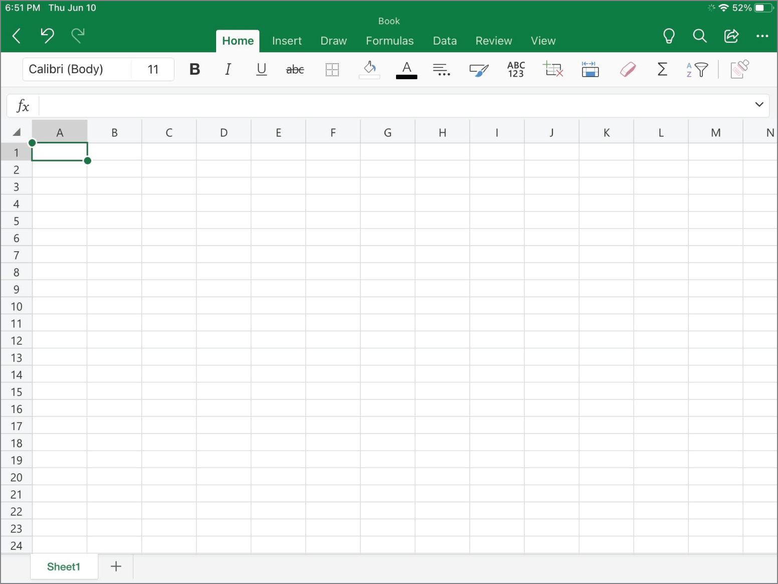
FIGURE 2.11 A blank workbook on a tablet
The selected cell, cell A1 in Figure 2.11, has handles in the upper-left and lower-right corners. To select a single cell, simply tap it. To expand the range, drag one of the handles. When you expand a range, Excel displays a context menu above or below the selected range containing often used commands. To see the context menu for a single cell, long press the cell.
To edit a cell, double-tap the cell to enter Edit mode. You can edit directly in the cell or tap in the Formula bar and make your changes there. When you enter Edit mode, the onscreen keyboard will appear. Another way to edit a cell is to long press to get the context menu and tap the Edit control.
To commit your edits to the cell, you can tap return on the onscreen keyboard, tap another cell, or tap the check mark control to the right of the Formula bar. There is also a red x control to the right of the Formula bar to exit Edit mode without committing your changes.
Entering formulas on a tablet
The Formulas tab on the Ribbon contains a control for each of the formula categories you're used to from desktop Excel. Tapping one of these controls presents a scrollable menu with all the functions in that category. The Formulas tab also has an AutoSum control that displays a menu of common functions and a Recent control that displays a menu of functions you've used recently.
Another way to enter formulas is by tapping the fx control to the left of the Formula bar. It displays recently used functions at the top and a menu of function categories and works similarly to the buttons on Formulas tab on the Ribbon.
Yet a third way to enter a formula is to simply type an equal sign. With this method, you can type the first letter of the worksheet function you want and a menu with all the functions that begin with that letter is displayed. Or you can type the entire worksheet function, but you may find that tedious. When you type an equal sign or select a function, Excel is in Point mode and tapping cells adds their addresses to the formula, just as in desktop Excel.
Figure 2.12 shows a cell with an INDEX worksheet function in it. When you select a function from a menu, the arguments are shown as buttons. You can tap the buttons to select cells or enter values for that argument.
In this example, the first argument was completed by tapping B3 and dragging the handle down to B7. Then the second argument button was selected and is shown slightly darker than the unselected argument buttons. While you wouldn't want to build a large spreadsheet using these methods, Excel has provided a very nice interface for entering a formula or two.
Introducing the Draw Ribbon
On mobile devices, the Draw tab on the Ribbon is shown by default. It contains drawing controls like pens, pencils, and highlighters for drawing in Excel. Like shapes and illustrations, drawn objects are on the drawing layer above the cells and aren't inside any particular cell.
You can draw a shape and convert it into an actual shape using Draw ➪ Convert ➪ Ink to Shape. Use the selection tool to select the drawing and click the Ink to Shape control or the lightning bolt that appears next to the shape. Figure 2.13 shows a crudely drawn circle converted to an oval shape.

FIGURE 2.12 Function arguments are displayed as buttons.
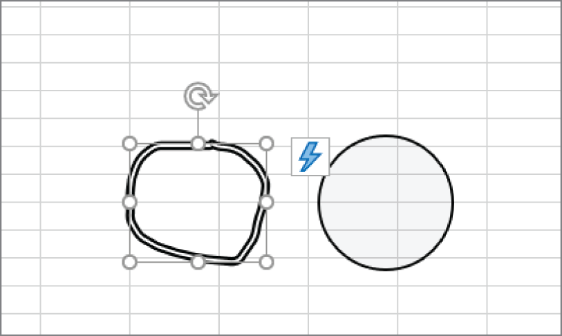
FIGURE 2.13 Convert a drawn shape into a native shape.
The Draw tab on the Ribbon contains a special pen called an Action Pen. The Action Pen lets you handwrite text and formulas in Excel and converts them after a short pause. To enter a formula with the Action Pen, select the cell first, then click the Action Pen and start writing. Figure 2.14 shows the formula =1+2 handwritten in a cell using the Action Pen and Figure 2.15 shows the result after a brief pause.

FIGURE 2.14 Handwrite a formula with the Action Pen.
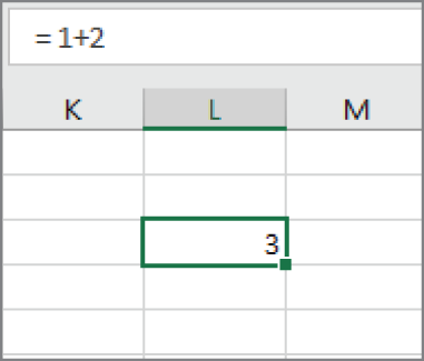
FIGURE 2.15 Excel converts a handwritten formula into an actual formula in the cell.