CHAPTER 1
Introducing Excel
This chapter is an introductory overview of Excel 2022. If you're already familiar with a previous version of Excel, reading (or at least skimming) this chapter is still a good idea.
Understanding What Excel Is Used For
Excel is the world's most widely used spreadsheet software and is part of the Microsoft Office suite. Other spreadsheet software is available, but Excel is by far the most popular and has been the world standard for many years.
Much of the appeal of Excel is its versatility. Excel's forte, of course, is performing numerical calculations, but Excel is also useful for nonnumeric applications. Here are just a few uses for Excel:
- Crunching numbers Create budgets, tabulate expenses, analyze survey results, and perform just about any type of financial analysis you can think of.
- Creating charts Create a variety of highly customizable charts.
- Organizing lists Use the row-and-column layout to store lists efficiently.
- Manipulating text Clean up and standardize text-based data.
- Accessing other data Import data from a variety of sources such as databases, text files, web pages, and many others.
- Creating graphical dashboards Summarize a large amount of business information in a concise format.
- Creating graphics and diagrams Use shapes and illustrations to create professional-looking diagrams.
- Automating complex tasks Perform a tedious task with a single mouse click with Excel's macro capabilities.
Understanding Workbooks and Worksheets
An Excel file is called a workbook. You can have as many workbooks open as you need, and each one appears in its own window. By default, Excel workbooks use an .xlsx file extension.
The tabs in a workbook are called worksheets. Each workbook contains one or more worksheets, and each worksheet consists of individual cells. Each cell can contain a number, a formula, or text. A worksheet also has an invisible drawing layer, which holds charts, images, and diagrams. Objects on the drawing layer sit over the top of the cells, but they are not in the cells like a number or formula. You switch to a different worksheet by clicking its tab at the bottom of the workbook window. In addition, a workbook can store chart sheets: a chart sheet displays a single chart and is accessible by clicking a tab.
Don't be intimidated by all the different elements that appear within Excel's window. You don't need to know what all of them mean to use Excel effectively. And after you become familiar with the various parts, it all starts to make sense and you'll feel right at home.
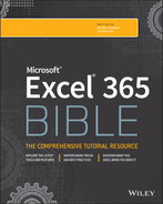
Figure 1.1 shows you the more important bits and pieces of Excel. As you look at the figure, refer to Table 1.1 for a brief explanation of the items shown.
Moving around a Worksheet
This section describes various ways to navigate the cells in a worksheet.
Every worksheet consists of rows (numbered 1 through 1,048,576) and columns (labeled A through XFD). Column labeling works like this: After column Z comes column AA, which is followed by AB, AC, and so on. After column AZ comes BA, BB, and so on. After column ZZ is AAA, AAB, and so on.
The intersection of a row and a column is a single cell, and each cell has a unique address made up of its column letter and row number. For example, the address of the upper-left cell is A1. The address of the cell at the lower right of a worksheet is XFD1048576.
At any given time, one cell is the active cell. The active cell is the cell that accepts keyboard input, and its contents can be edited. You can identify the active cell by its darker border, as shown in Figure 1.2. If more than one cell is selected, the dark border surrounds the entire selection, and the active cell is the light-colored cell within the border. Its address appears in the Name box. Depending on the technique you use to navigate through a workbook, you may or may not change the active cell when you navigate.
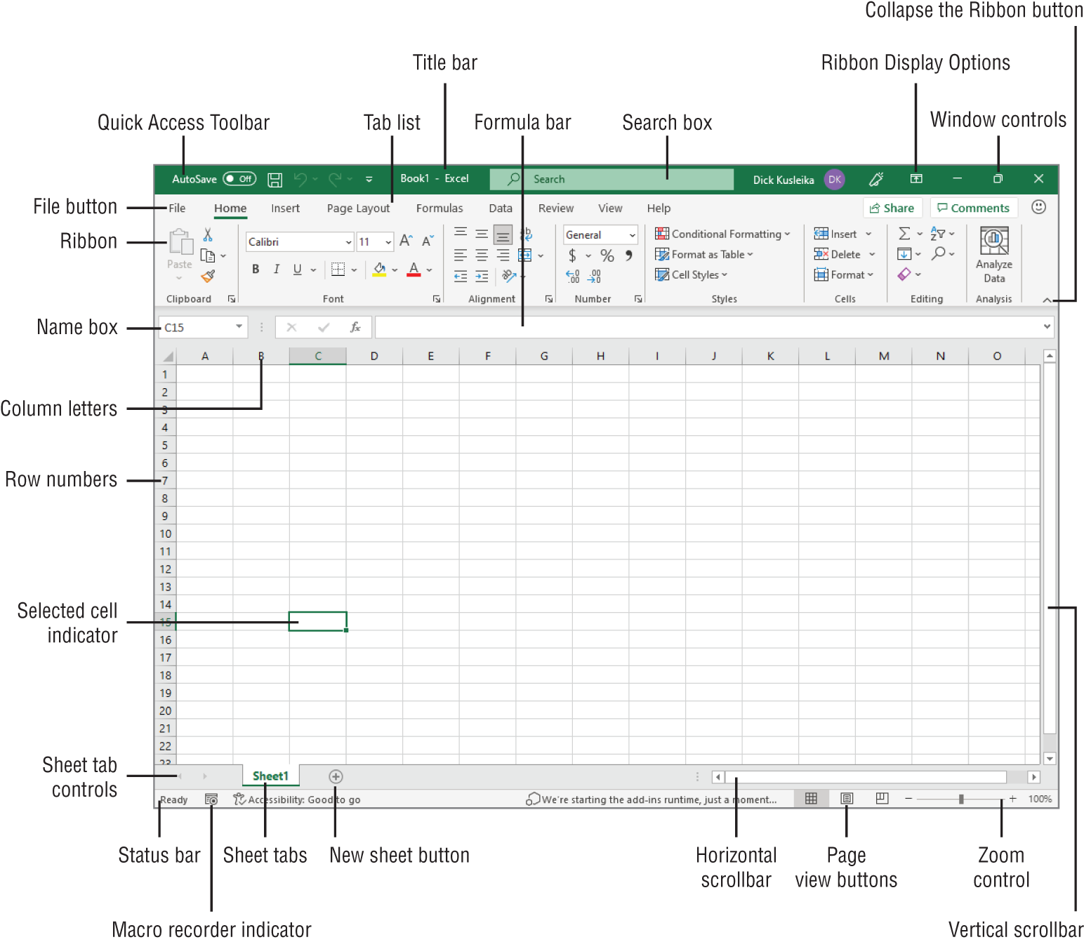
FIGURE 1.1 The Excel screen has many useful elements that you will use often.
TABLE 1.1 Parts of the Excel Screen That You Need to Know
| Name | Description |
|---|---|
| Collapse the Ribbon button | Click this button to hide the Ribbon temporarily. Double-click any Ribbon tab to make the Ribbon remain visible. Ctrl+F1 is the shortcut key that does the same task. |
| Column letters | Letters range from A to XFD—one for each of the 16,384 columns in the worksheet. You can click a column heading to select an entire column or click between the column letters and drag to change the column width. |
| File button | Click this button to open Backstage view, which contains many options for working with your document (including printing) and setting Excel options. |
| Formula bar | When you enter information or formulas into a cell, it appears in this bar. |
| Horizontal scrollbar | Use this tool to scroll the sheet horizontally. |
| Macro recorder indicator | Click to start recording a Visual Basic for Applications (VBA) macro. The icon changes while your actions are being recorded. Click again to stop recording. |
| Name box | This box displays the active cell address or the name of the selected cell, range, or object. |
| New sheet button | Add a new worksheet by clicking the New sheet button (which is displayed after the last sheet tab). |
| Page view buttons | Click these buttons to change the way the worksheet is displayed. |
| Quick Access Toolbar | This customizable toolbar holds commonly used commands. The Quick Access Toolbar is always visible, regardless of which tab is selected. |
| Ribbon | This is the main location for Excel commands. Clicking an item in the tab list changes the Ribbon that is displayed. |
| Ribbon Display Options | A drop-down control that offers three options related to displaying the Ribbon. |
| Row numbers | Numbers range from 1 to 1,048,576—one for each row in the worksheet. You can click a row number to select an entire row or click between the row numbers and drag to change the row height. |
| Search box | Use this control to find commands or have Excel issue a command automatically. Alt+Q is the shortcut to access the Search box. |
| Selected cell indicator | This dark outline indicates the currently selected cell or range of cells. (There are 17,179,869,184 cells on each worksheet.) |
| Sheet tabs | Each of these notebook-like tabs represents a different sheet in the workbook. A workbook can have any number of sheets, and each sheet has its name displayed in a sheet tab. |
| Sheet tab controls | Use these buttons to scroll the sheet tabs to display tabs that aren't visible. You can also right-click to get a list of sheets. |
| Status bar | This bar displays various messages as well as summary information about the range of cells selected. Right-click the status bar to change which messages are displayed. |
| Tab list | Use these commands to display a different Ribbon. |
| Title bar | This displays the name of the program and the name of the current workbook. It also holds the Quick Access Toolbar (on the left), the Search box, and some control buttons that you can use to modify the window (on the right). |
| Vertical scrollbar | Use this tool to scroll the sheet vertically. |
| Window controls | There are three controls for minimizing the current window, maximizing or restoring the current window, and closing the current window, which are common to virtually all Windows applications. |
| Zoom control | Use this to zoom your worksheet in and out. |
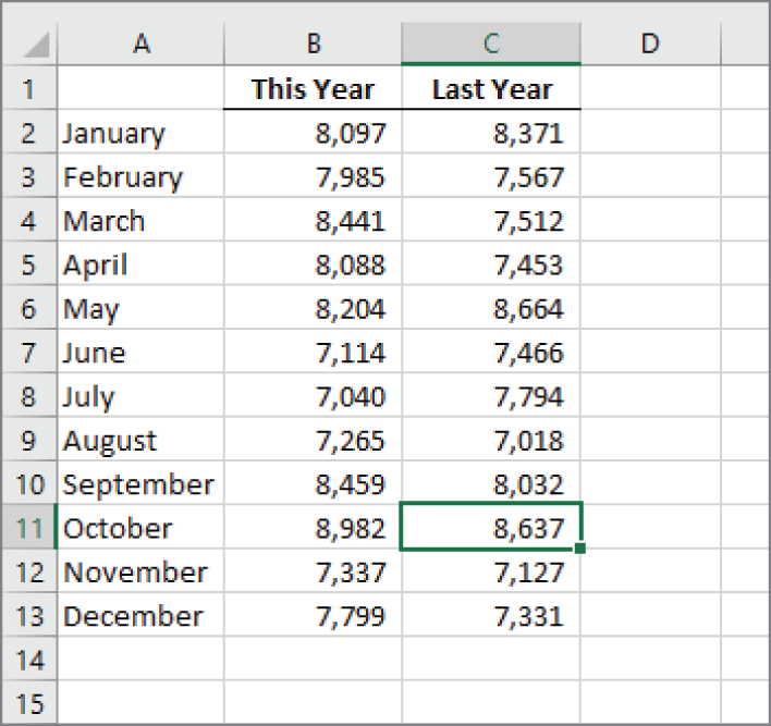
FIGURE 1.2 The active cell is the one with the dark border—in this case, cell C11.
The row and column headings of the active cell appear in a different color to make it easier to identify the row and column of the active cell.
Navigating with your keyboard
Not surprisingly, you can use the standard navigational keys on your keyboard to move around a worksheet. These keys work just as you'd expect: the down arrow moves the active cell down one row, the right arrow moves it one column to the right, and so on. PgUp and PgDn move the active cell up or down one full window. (The actual number of rows moved depends on the number of rows displayed in the window.)
The Num Lock key on your keyboard controls the way the keys on the numeric keypad behave. When Num Lock is on, the keys on your numeric keypad generate numbers. Many keyboards have a separate set of navigation (arrow) keys located to the left of the numeric keypad. The state of the Num Lock key doesn't affect these keys.
Table 1.2 summarizes all the worksheet movement keys available in Excel.
TABLE 1.2 Excel Worksheet Movement Keys
| Key | Action |
|---|---|
| Up arrow (↑) or Shift+Enter | Moves the active cell up one row |
| Down arrow (↓) or Enter | Moves the active cell down one row |
| Left arrow (←) or Shift+Tab | Moves the active cell one column to the left |
| Right arrow (→) or Tab | Moves the active cell one column to the right |
| PgUp | Moves the active cell up one screen |
| PgDn | Moves the active cell down one screen |
| Alt+PgDn | Moves the active cell right one screen |
| Alt+PgUp | Moves the active cell left one screen |
| Ctrl+Backspace | Scrolls the screen so that the active cell is visible |
| Ctrl+Home | Moves the active cell to A1 |
| Ctrl+End | Moves the active cell to the bottom-rightmost cell on the worksheet's used range |
| ↑* | Scrolls the screen up one row (active cell does not change) |
| ↓* | Scrolls the screen down one row (active cell does not change) |
| ←* | Scrolls the screen left one column (active cell does not change) |
| →* | Scrolls the screen right one column (active cell does not change) |
* With Scroll Lock on
Navigating with your mouse
To change the active cell by using the mouse, just click another cell and it becomes the active cell. If the cell that you want to activate isn't visible in the workbook window, you can use the scrollbars to scroll the window in any direction. To scroll one cell, click either of the arrows on the scrollbar. To scroll by a complete screen, click either side of the scrollbar's scroll box. To scroll faster, drag the scroll box or right-click anywhere on the scrollbar for a menu of shortcuts.
Press Ctrl while you use the mouse wheel to zoom the worksheet. If you prefer to use the mouse wheel to zoom the worksheet without pressing Ctrl, choose File ➪ Options and select the Advanced section. Place a check mark next to the Zoom on Roll with IntelliMouse check box.
Using the scrollbars or scrolling with your mouse doesn't change the active cell. It simply scrolls the worksheet. To change the active cell, you must click a new cell after scrolling.
Using the Ribbon
The Ribbon is the primary way of interacting with Excel other than entering data into cells. The words above the icons are known as tabs: the Home tab, the Insert tab, and so on. The term Ribbon is used in two different ways: when you click a tab, you are said to be displaying a different Ribbon and the whole structure of tabs, groups, and controls is known as the Ribbon.
The Ribbon can be either hidden or visible. It's your choice. To toggle the Ribbon's visibility, press Ctrl+F1 (or double-click a tab at the top). If the Ribbon is hidden, it temporarily appears when you click a tab and hides itself when you click in the worksheet. The title bar has a control named Ribbon Display Options (next to the Minimize button). Click the control and choose one of three Ribbon options: Auto-Hide Ribbon, Show Tabs, or Show Tabs and Commands.
Ribbon tabs
The commands available on the Ribbon vary, depending upon which tab is selected. The Ribbon is arranged into groups of related commands. Here's a quick overview of Excel's tabs:
- Home You'll probably spend most of your time with the Home tab selected. This tab contains the basic Clipboard commands, formatting commands, style commands, commands to insert and delete rows or columns, plus an assortment of worksheet editing commands.
- Insert Select this tab when you need to insert something into a worksheet—a table, a diagram, a chart, a symbol, and so on.
- Page Layout This tab contains commands that affect the overall appearance of your worksheet, including some settings that deal with printing.
- Formulas Use this tab to insert a formula, name a cell or a range, access the formula auditing tools, or control the way Excel performs calculations.
- Data Excel's data-related commands are on this tab, including data validation and sorting commands.
- Review This tab contains tools to check spelling, translate words, add comments, or protect sheets.
- View The View tab contains commands that control various aspects of how a sheet is viewed. Some commands on this tab are also available in the status bar.
- Developer This tab isn't visible by default. It contains commands that are useful for programmers. To display the Developer tab, choose File ➪ Options and then select Customize Ribbon. In the Customize the Ribbon section on the right, make sure that Main Tabs is selected in the drop-down control and place a check mark next to Developer.
- Help This tab provides ways to get help, make suggestions, and access other aspects of Microsoft's community.
- Add-Ins This tab is visible only if you loaded an older workbook or add-in that customizes the menu or toolbars. Because the old menus and toolbars were replaced by the Ribbon, these user interface customizations appear on the Add-Ins tab.
The preceding list contains the standard Ribbon tabs. Excel may display additional Ribbon tabs based on what's selected or resulting from add-ins that are installed.
The appearance of the commands on the Ribbon varies, depending on the width of the Excel window. When the Excel window is too narrow to display everything, the commands adapt; some of them might seem to be missing, but the commands are still available. Figure 1.3 shows the Home tab of the Ribbon with all controls fully visible. Figure 1.4 shows the Ribbon when Excel's window is made narrower. Notice that some of the descriptive text is gone, but the icons remain. Figure 1.5 shows the extreme case when the window is made very narrow. Most groups display a single icon; however, if you click the icon, all the group commands are available to you.

FIGURE 1.3 The Home tab of the Ribbon
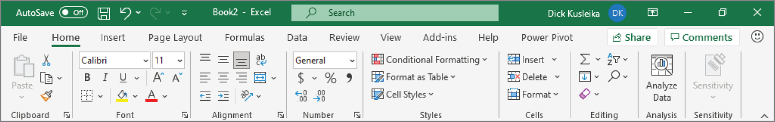
FIGURE 1.4 The Home tab when Excel's window is made narrower
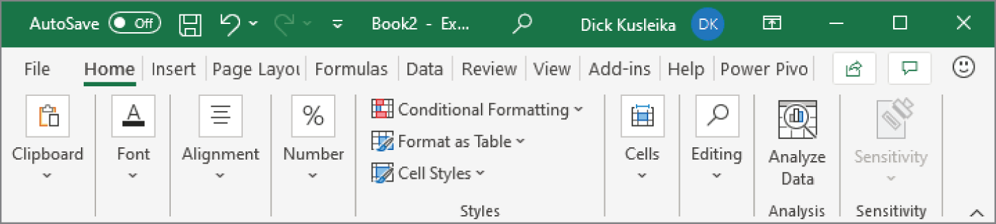
FIGURE 1.5 The Home tab when Excel's window is made very narrow
Contextual tabs
In addition to the standard tabs, Excel includes contextual tabs. Whenever an object (such as a chart, a table, or an illustration) is selected, specific tools for working with that object are made available on the Ribbon.
Figure 1.6 shows the contextual tabs that appear when a chart is selected. In this case, it has two contextual tabs: Chart Design and Format. When contextual tabs appear, you can, of course, continue to use all the other tabs.
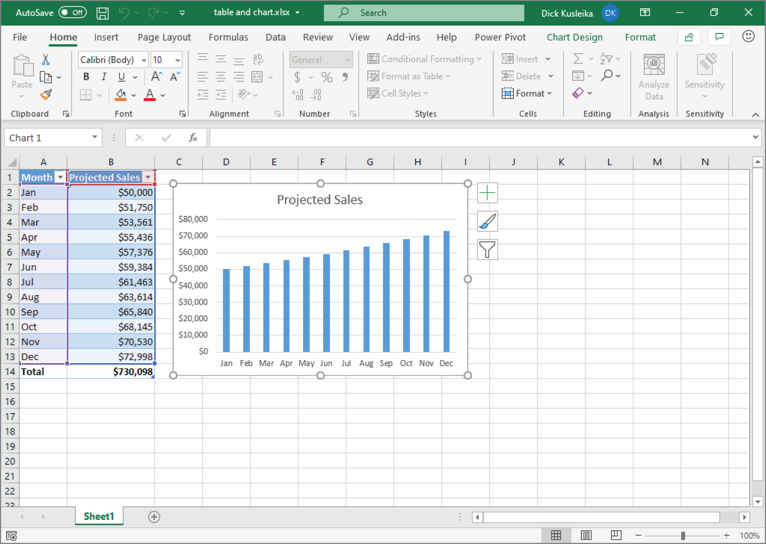
FIGURE 1.6 When you select an object, contextual tabs contain tools for working with that object.
Types of commands on the Ribbon
When you hover your mouse pointer over a Ribbon command, you'll see a ScreenTip that contains the command's name and a brief description. For the most part, the commands on the Ribbon work just as you would expect. You'll find several different styles of commands on the Ribbon.
- Simple buttons Click the button, and it does its thing. An example of a simple button is the Increase Font Size button in the Font group of the Home tab. Some buttons perform the action immediately; others display a dialog box so that you can enter additional information. Button controls may or may not be accompanied by a descriptive label.
- Toggle buttons A toggle button is clickable and conveys some type of information by displaying two different colors. An example is the Bold button in the Font group of the Home tab. If the active cell isn't bold, the Bold button displays in its normal color. If the active cell is already bold, the Bold button displays a different background color. If you click the Bold button, it toggles the Bold attribute for the selection.
- Simple drop-downs If the Ribbon command has a small down arrow, the command is a drop-down menu. Click it, and additional commands appear below it. An example is the Conditional Formatting command in the Styles group of the Home tab. When you click this control, you see several options related to conditional formatting. Style galleries, like the Data Types gallery on the Data tab, also have drop-down arrows to reveal more styles if they are available.
- Split buttons A split button control combines a one-click button with a drop-down. If you click the button part, the command is executed. If you click the drop-down part (a down arrow), you choose from a list of related commands. An example of a split button is the Merge & Center command in the Alignment group of the Home tab (see Figure 1.7). Clicking the left part of this control merges and centers text in the selected cells. If you click the arrow part of the control (on the right), you get a list of commands related to merging cells.
- Check boxes A check box control turns something on or off. An example is the Gridlines control in the Show group of the View tab. When the Gridlines check box is checked, the sheet displays gridlines. When the control isn't checked, the gridlines don't appear.
- Spin buttons Excel's Ribbon has only one spin button control: the Scale to Fit group of the Page Layout tab. Click the top part of the spin button to increase the value; click the bottom part of the spin button to decrease the value.
Some of the Ribbon groups contain a small icon in the bottom-right corner, known as a dialog box launcher. For example, if you examine the groups on the Home tab, you find dialog box launchers for the Clipboard, Font, Alignment, and Number groups—but not the Styles, Cells, and Editing groups. Click the icon, and Excel displays a dialog box or task pane. The dialog box launchers often provide options that aren't available on the Ribbon.
Accessing the Ribbon by using your keyboard
At first glance, you may think that the Ribbon is completely mouse centric. After all, the commands don't display the traditional underlined letter to indicate the Alt+keystrokes. But in fact, the Ribbon is very keyboard friendly. The trick is to press the Alt key to display the pop-up keytips. Each Ribbon control has a letter (or series of letters) that you type to issue the command.
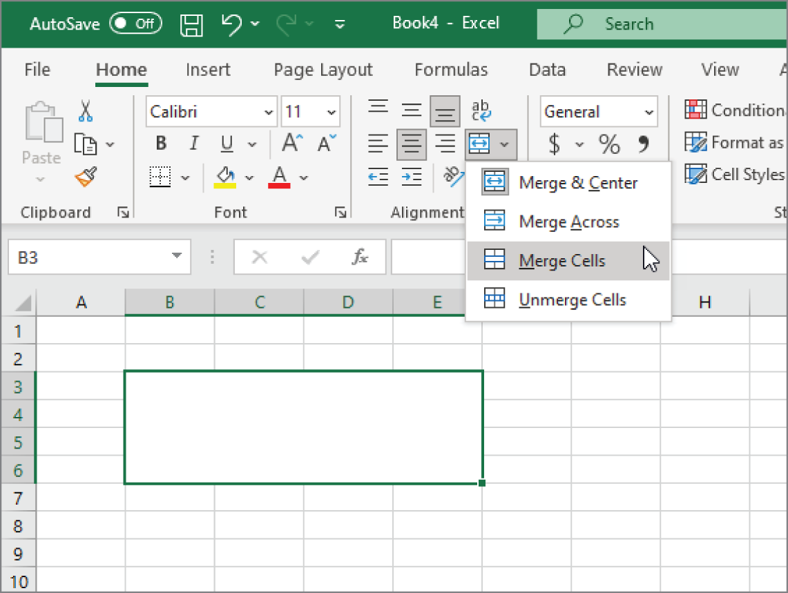
FIGURE 1.7 The Merge & Center command is a split button control.
Figure 1.8 shows how the Home tab looks after you press the Alt key to display the keytips and then the H key to display the keytips for the Home tab. If you press one of the keytips, the screen then displays more keytips. For example, to use the keyboard to align the cell contents to the left, press Alt, followed by H (for Home), and then AL (for Align Left).
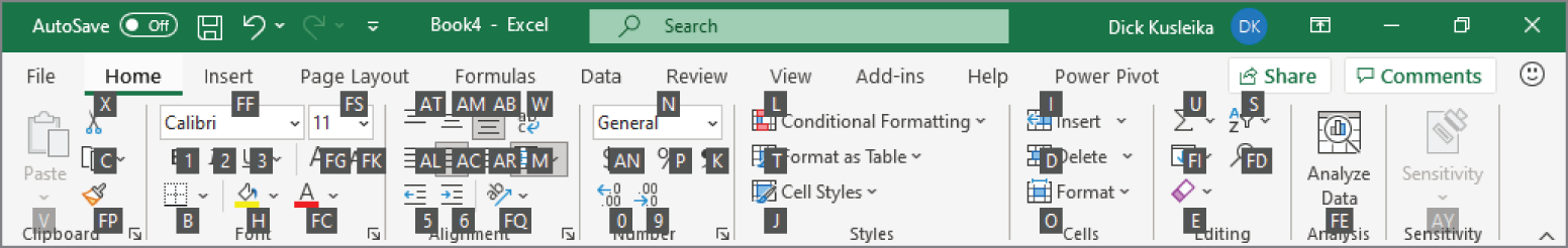
FIGURE 1.8 Pressing Alt displays the keytips.
Nobody will memorize all of these keys, but if you're a keyboard fan, it takes just a few times before you memorize the keystrokes required for commands that you use frequently.
After you press Alt, you can also use the left- and right-arrow keys to scroll through the tabs. When you reach the proper tab, press the down arrow to enter the Ribbon. Then use left- and right-arrow keys to scroll through the Ribbon commands. If you hold down the Ctrl key while in the Ribbon, the left and right arrows will jump to the first control in the previous or next group, respectively. When you reach the command you need, press Enter to execute it. This method isn't as efficient as using the keytips, but it's a quick way to take a look at the commands available.
Using Shortcut Menus
In addition to the Ribbon, Excel features many shortcut menus, which you access by right-clicking just about anything within Excel. Shortcut menus don't contain every relevant command, just those that are most commonly used for whatever is selected.
As an example, Figure 1.9 shows the shortcut menu that appears when you right-click a cell in a table. The shortcut menu appears at the mouse-pointer position, which makes selecting a command fast and efficient. The shortcut menu that appears depends on what you're doing at the time. For example, if you're working with a chart, the shortcut menu contains commands that are pertinent to the selected chart element.
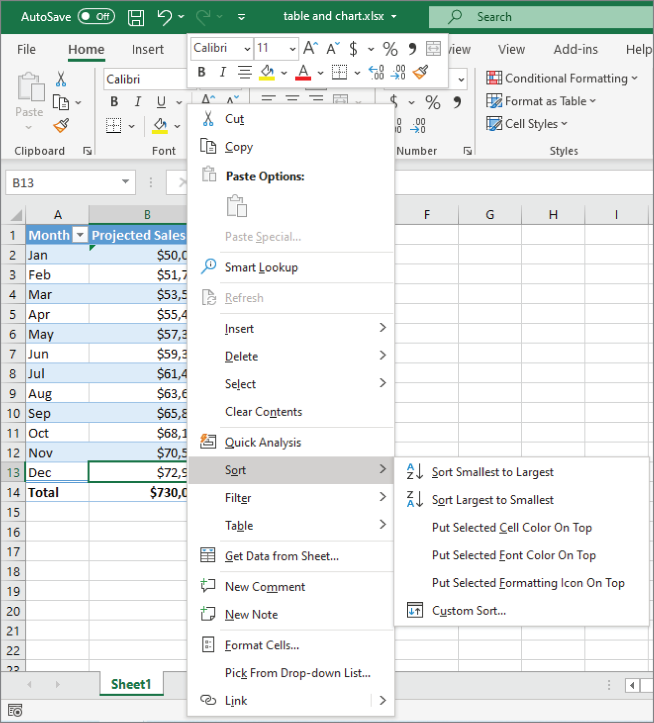
FIGURE 1.9 Right-click to display a shortcut menu of commands you're most likely to use.
The box above the shortcut menu—the Mini toolbar—contains commonly used tools from the Home tab. The Mini toolbar was designed to reduce the distance your mouse has to travel around the screen. Just right-click, and common formatting tools are near your mouse pointer. The Mini toolbar is particularly useful when a tab other than Home is displayed. If you use a tool on the Mini toolbar, the toolbar remains displayed in case you want to perform other formatting on the selection.
Customizing Your Quick Access Toolbar
The Ribbon is efficient, but many users prefer to have certain commands available at all times without having to click a tab. The solution is to customize your Quick Access Toolbar. Typically, the Quick Access Toolbar appears on the left side of the title bar, above the Ribbon. Alternatively, you can display the Quick Access Toolbar below the Ribbon; just right-click the Quick Access Toolbar and choose Show Quick Access Toolbar Below the Ribbon.
Displaying the Quick Access Toolbar below the Ribbon provides a bit more room for icons, but it also means that you see one less row of your worksheet.
By default, the Quick Access Toolbar contains four tools: AutoSave, Save, Undo, and Redo. You can customize the Quick Access Toolbar by adding other commands that you use often or removing the default controls. To add a command from the Ribbon to your Quick Access Toolbar, right-click the command and choose Add to Quick Access Toolbar. If you click the down arrow to the right of the Quick Access Toolbar, you will see a drop-down menu with some additional commands that you might want to place in your Quick Access Toolbar.
Excel has quite a few commands (mostly obscure ones) that aren't available on the Ribbon. In most cases, the only way to access these commands is to add them to your Quick Access Toolbar. Right-click the Quick Access Toolbar and choose Customize Quick Access Toolbar. You see the Excel Options dialog box, shown in Figure 1.10. This section of the Excel Options dialog box is your one-stop shop for Quick Access Toolbar customization.

FIGURE 1.10 Add new icons to your Quick Access Toolbar by using the Quick Access Toolbar section of the Excel Options dialog box.
Working with Dialog Boxes
Many Excel commands display a dialog box, which is simply a way of getting more information from you. For example, if you choose Review ➪ Protect ➪ Protect Sheet, Excel can't carry out the command until you tell it what parts of the sheet you want to protect. Therefore, it displays the Protect Sheet dialog box, shown in Figure 1.11.
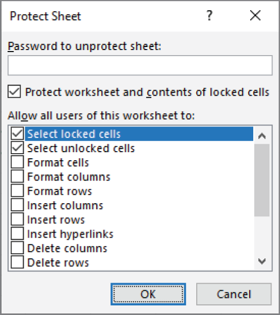
FIGURE 1.11 Excel uses a dialog box to get additional information about a command.
Excel dialog boxes vary in the way they work. You'll find two types of dialog boxes.
- Typical dialog box A modal dialog box takes the focus away from the spreadsheet. When this type of dialog box is displayed, you can't do anything in the worksheet until you dismiss the dialog box. Clicking OK performs the specified actions and clicking Cancel (or pressing Esc) closes the dialog box without taking any action. Most Excel dialog boxes are this type.
- Stay-on-top dialog box A modeless dialog box works in a manner similar to a toolbar. When a modeless dialog box is displayed, you can continue working in Excel, and the dialog box remains open. Changes made in a modeless dialog box take effect immediately. An example of a modeless dialog box is the Find and Replace dialog box. You can leave this dialog box open while you continue to use your worksheet. A modeless dialog box has a Close button but no OK button.
Most people find working with dialog boxes to be quite straightforward and natural. If you've used other programs, you'll feel right at home. You can manipulate the controls either with your mouse or directly from the keyboard.
Navigating dialog boxes
Navigating dialog boxes is generally easy—you simply click the control that you want to activate.
Although dialog boxes were designed with mouse users in mind, you can also use the keyboard. Every dialog box control has text associated with it, and this text always has one underlined letter (called a hot key or an accelerator key). You can access the control from the keyboard by pressing Alt and then the underlined letter. You can also press Tab to cycle through all the controls on a dialog box. Pressing Shift+Tab cycles through the controls in reverse order.
Using tabbed dialog boxes
Several Excel dialog boxes are “tabbed” dialog boxes; that is, they include notebook-like tabs, each of which is associated with a different panel.
When you select a tab, the dialog box changes to display a new panel containing a new set of controls. The Format Cells dialog box, shown in Figure 1.12, is a good example. It has six tabs, which makes it functionally equivalent to six different dialog boxes.
Tabbed dialog boxes are quite convenient because you can make several changes in a single dialog box. After you make all your setting changes, click OK or press Enter.
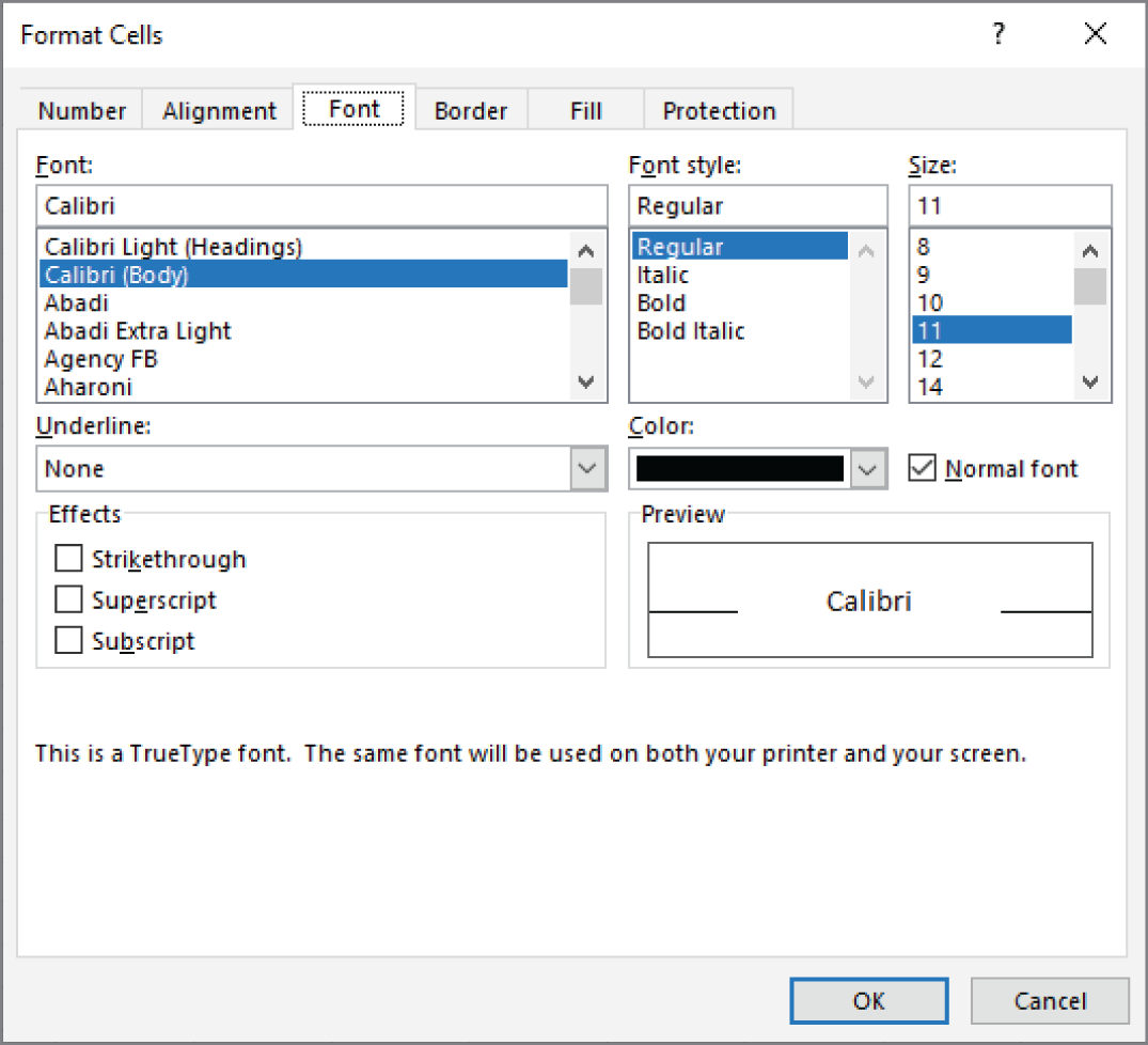
FIGURE 1.12 Use the dialog box tabs to select different functional areas of the dialog box.
Using Task Panes
Another user interface element is the task pane. Task panes appear automatically in response to several commands. For example, to work with a picture that you've inserted, right-click the image and choose Format Picture. Excel responds by displaying the Format Picture task pane, shown in Figure 1.13. The task pane is similar to a dialog box except that you can keep it visible as long as you like.
Many of the task panes are complex. The Format Picture task pane has four icons along the top. Clicking an icon changes the command lists displayed next. Click an item in a command list and it expands to show the options.
There's no OK button in a task pane. When you're finished using a task pane, click the Close button (X) in the upper-right corner.
By default, a task pane is docked on the right side of the Excel window, but you can move it anywhere you like by clicking its title bar and dragging. Excel remembers the last position, so the next time you use that task pane, it will be right where you left it. To re-dock the task pane, double-click the task pane's title bar.
Creating Your First Excel Workbook
This section presents an introductory, hands-on session with Excel. If you haven't used Excel, you may want to follow along on your computer to get a feel for how this software works.
In this example, you create a simple monthly sales projection table plus a chart that depicts the data.
Getting started on your worksheet
Start Excel and make sure you have an empty workbook displayed. To create a new, blank workbook, press Ctrl+N (the shortcut key for File ➪ New ➪ Blank Workbook). Enter some sales projections in the new workbook.
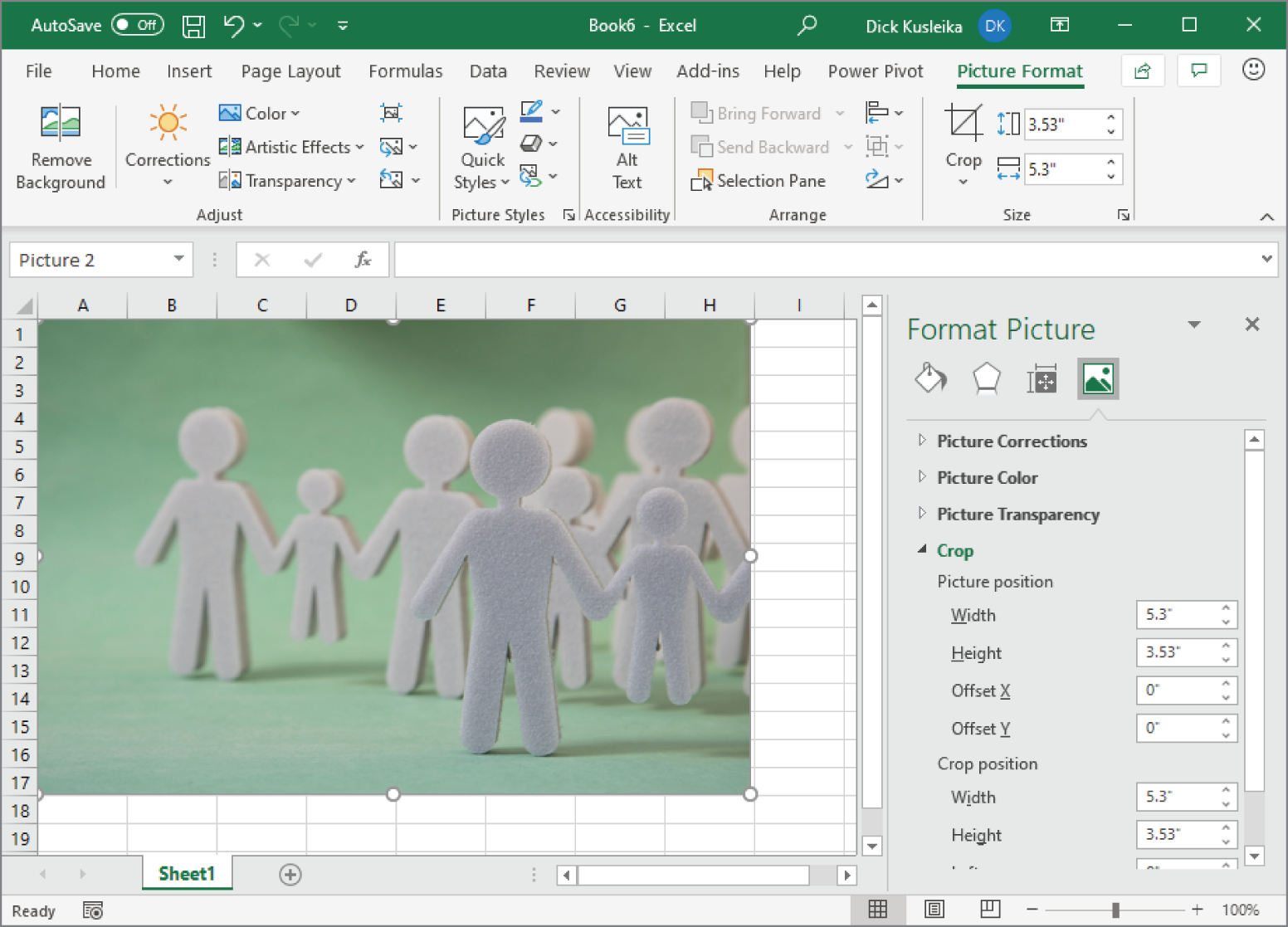
FIGURE 1.13 The Format Picture task pane, docked on the right side of the window
The sales projections will consist of two columns of information. Column A will contain the month names, and column B will store the projected sales numbers. You start by entering some descriptive titles into the worksheet. Here's how to begin:
- Select cell A1 (the upper-left cell in the worksheet) by using the navigation (arrow) keys, if necessary. The Name box displays the cell's address.
- Type Month into cell A1 and press Enter. Depending on your setup, either Excel moves the selection to a different cell or the pointer remains in cell A1.
- Select cell B1, type Projected Sales, and press Enter. The text extends beyond the cell width, but don't worry about that for now.
Filling in the month names
In this step, you enter the month names in column A.
- Select cell A2 and type Jan (an abbreviation for January). At this point, you can enter the other month name abbreviations manually, or you can let Excel do some of the work by taking advantage of the AutoFill feature.
- Make sure that cell A2 is selected. Notice that the active cell is displayed with a heavy outline. At the bottom-right corner of the outline, you'll see a small square known as the fill handle. Move your mouse pointer over the fill handle, click, and drag down until you've highlighted from cell A2 down to cell A13.
- Release the mouse button, and Excel automatically fills in the month names.
Your worksheet should resemble the one shown in Figure 1.14.

FIGURE 1.14 Your worksheet after you've entered the column headings and month names
Entering the sales data
Next, you provide the sales projection numbers in column B. Assume that January's sales are projected to be $50,000 and that sales will increase by 3.5 percent in each subsequent month.
- Select cell B2 and type 50000, the projected sales for January. You could type a dollar sign and comma to make the number more legible, but you do the number formatting a bit later.
- To enter a formula to calculate the projected sales for February, move to cell B3 and type the following:
=B2*103.5%
When you press Enter, the cell displays
51750. The formula returns the contents of cell B2, multiplied by 103.5%. In other words, February sales are projected to be 103.5% of the January sales—a 3.5% increase. - The projected sales for subsequent months use a similar formula, but rather than retype the formula for each cell in column B, take advantage of the AutoFill feature. Make sure that cell B3 is selected. Click the cell's fill handle, drag down to cell B13, and release the mouse button.
At this point, your worksheet should resemble the one shown in Figure 1.15. Keep in mind that, except for cell B2, the values in column B are calculated with formulas. To demonstrate, try changing the projected sales value for the initial month, January (in cell B2). You'll find that the formulas recalculate and return different values. All these formulas depend on the initial value in cell B2.
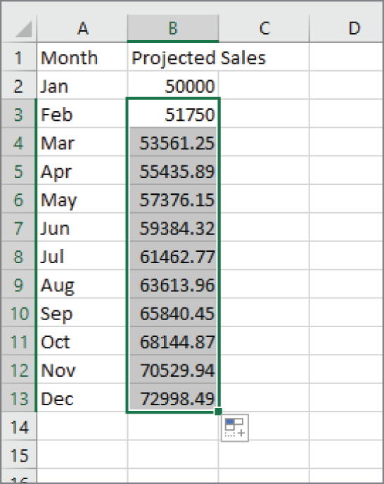
FIGURE 1.15 Your worksheet after you've created the formulas
Formatting the numbers
The values in the worksheet are difficult to read because they aren't formatted. In this step, you apply a number format to make the numbers easier to read and more consistent in appearance.
- Select the numbers by clicking cell B2 and dragging down to cell B13. Don't drag the fill handle this time, though, because you're selecting cells, not filling a range.
- Access the Ribbon and choose Home. In the Number group, click the drop-down Number Format control (it initially displays General), and select Currency from the list. The numbers now display with a currency symbol and two decimal places. That's much better, but the decimal places aren't necessary for this type of projection.
- Make sure that the range B2:B13 is selected, choose Home ➪ Number, and click the Decrease Decimal button. One of the decimal places disappears. Click that button a second time and the values are displayed with no decimal places.
Making your worksheet look a bit fancier
At this point, you have a functional worksheet, but it could use some help in the appearance department. Converting this range to an “official” (and attractive) Excel table is a snap.
- Activate any cell within the range A1:B13.
- Choose Insert ➪ Tables ➪ Table. Excel displays the Create Table dialog box to make sure that it guessed the range properly.
- Click OK to close the Create Table dialog box. Excel applies its default table formatting and displays its Table Design contextual tab.
Your worksheet should look like Figure 1.16.

FIGURE 1.16 Your worksheet after you've converted the range to a table
If you don't like the default table style, just select another one from the Table Design ➪ Table Styles group. Notice that you can get a preview of different table styles by moving your mouse over the Ribbon. When you find one you like, click it, and the style will be applied to your table.
Summing the values
The worksheet displays the monthly projected sales, but what about the total projected sales for the year? Because this range is a table, it's simple.
- Activate any cell in the table.
- Choose Table Design ➪ Table Style Options ➪ Total Row. Excel automatically adds a new row to the bottom of your table, including a formula that calculates the total of the Projected Sales column.
- If you'd prefer to see a different summary formula (for example, average), click cell B14 and choose a different summary formula from the drop-down list.
Creating a chart
How about a chart that shows the projected sales for each month?
- Activate any cell in the table.
- Choose Insert ➪ Charts ➪ Recommended Charts. Excel displays some suggested chart type options.
- In the Insert Chart dialog box, click the second recommended chart (a column chart), and click OK. Excel inserts the chart in the center of the window. To move the chart to another location, click its border and drag it.
- Click the chart and choose a style using the Chart Design ➪ Chart Styles options.
Figure 1.17 shows the worksheet with a column chart. Your chart may look different, depending on the chart style you selected.
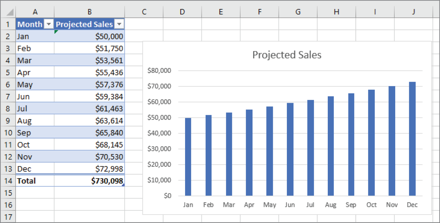
FIGURE 1.17 The table and chart
Printing your worksheet
Printing your worksheet is easy (assuming that you have a printer attached and that it works properly).
- Make sure that the chart isn't selected. If a chart is selected, the chart will print on a page by itself. To deselect the chart, just press Esc or click any cell.
- To make use of Excel's handy Page Layout view, click the Page Layout button on the right side of the status bar. Excel displays the worksheet page by page so that you can easily see how your printed output will look. In Page Layout view, you can tell immediately whether the chart is too wide to fit on one page. If the chart is too wide, click and drag a corner of the chart to resize it or just move the chart below the table of numbers. Click the Normal button to return to the default view.
- When you're ready to print, choose File ➪ Print. At this point, you can change some print settings. For example, you can choose to print in landscape rather than portrait orientation. Make the change, and you see the result in the preview window.
- When you're satisfied, click the large Print button in the upper-left corner. The page is printed, and you're returned to your workbook.
Saving your workbook
Until now, everything that you've done has occurred in your computer's memory. If the power should fail, all may be lost—unless Excel's AutoRecover feature happened to kick in. It's time to save your work to a file on your hard drive.
- Click the Save button on the Quick Access Toolbar. (This button looks like an old-fashioned floppy disk, popular in the previous century.) Because the workbook hasn't been saved yet and still has its default name, Excel responds with a Save this file dialog box that lets you choose the location for the workbook file. The Choose a Location drop-down lists some recently used locations, or you can click More options to see the Save as Backstage screen. From there, you can click Browse to navigate to any location on your computer.
- Click Browse. Excel displays the Save As dialog box.
- In the File Name field, enter a name (such as Monthly Sales Projection). If you like, you can specify a different location.
- Click Save or press Enter. Excel saves the workbook as a file. The workbook remains open so that you can work with it some more.
If you've followed along, you probably have realized that creating this workbook was not difficult. But, of course, you've barely scratched the surface of Excel. The remainder of this book covers these tasks (and many, many more) in much greater detail.