
CHAPTER 9
MICROSOFT ACCESS SQL
In this chapter I show you how to use Microsoft Access SQL for querying and managing databases without the help of Access wizards. I specifically show you two subsets of the Access SQL language, called DML and DDL.
If you’re new to database languages such as SQL, consider this chapter a prerequisite for Chapter 10, “Database Programming with ADO.” Even if you’ve worked with SQL before, you may find this chapter a refresher for Microsoft Access SQL syntax and common functionality.
INTRODUCTION TO ACCESS SQL
Most databases, including Microsoft Access, incorporate one or more data languages for querying information and managing databases. The most common of these data languages is SQL (Structured Query Language), which contains a number of commands for querying and manipulating databases. SQL commands are typically grouped into one of two categories known as data manipulation language (DML) commands and data definition language (DDL) commands.
Microsoft Access SQL follows a standard convention known as ANSI SQL, which is used by many database vendors, including Microsoft, Oracle, and IBM. Each manufacturer, however, incorporates its own proprietary language-based functions and syntax. Access SQL is no exception with key differences in reserved words and data types.
To demonstrate Access SQL, I use Access Queries in SQL View with Microsoft’s sample Northwind database that can be found by selecting Sample Templates under Available Templates, seen in Figure 9.1. As of this writing, you can also download the Access 2010 Northwind database from Microsoft here: http://office.microsoft.com/en-us/templates/CT010375241.aspx#ai:TC101114818|
FIGURE 9.1 Finding the Microsoft Access 2010 Northwind database.

![]()
You can bypass the default Northwind login form by holding down the Shift key while simultaneously opening the Northwind database file. To accomplish the same if this is the first time you are opening the Northwind database, or if it is not in a trusted location, you will need to hold down the Shift key while simultaneously clicking the Enable Content button from the Security Warning bar.
Building queries in Microsoft Access is much like the experience of building tables and forms in Access. Essentially, Microsoft provides wizards and graphical interfaces for building everything, including queries. In this chapter, I show you how to go beyond wizards to build your own queries using SQL!
To access the SQL window in Access, open a query by double-clicking it, or right-click it and select either Design View or Open. After the query is opened, right-click the query’s tab and select SQL View from the menu, which I’ve done for the Top Ten Orders by Sales Amount query in Figure 9.2.
FIGURE 9.2 Viewing the Top Ten Orders by Sales Amount query in SQL View.

SQL is not considered to be a full-fledged programming language like VBA, C, or Java. Genuine programming languages should, at minimum, contain facilities for creating variables, as well as structures for conditional logic branches and iteration through loops. Nevertheless, even without those facilities, SQL is a powerful language for asking the database questions (also known as querying).
Pronounced sequel, SQL was originally developed by IBM researchers in the 1970s. It has become the de facto database manipulation language for many database vendors. For database users, mastering SQL has become a sought-after skill set in the information technology world. Most persons who master the SQL language have no trouble finding well-paid positions.
To provide readability in the sections to come, I use a preferred syntax nomenclature for SQL:
• All SQL commands and reserved language keywords are in uppercase. For example, SELECT, FROM, WHERE, and AND are all Access SQL commands and reserved keywords.
• Even though Microsoft Access is not a case-sensitive application, table and column names used in SQL statements use the same case as defined in the database. For example, a column defined as EmployeeId is spelled EmployeeId in the SQL query.
• Table and column names that contain spaces must be enclosed in brackets. For example, the column name Customer Number must be referenced in SQL as [Customer Number]. Failure to do so will cause errors, or undesired results when executing your queries.
• A query can be written on a single line. For readability, I break SQL statements into logical blocks on multiple lines. For example, look at this SQL statement:
SELECT [Order Details].OrderID, SUM(CCur([UnitPrice]*[Quantity]*(1-[Discount])/100)
*100) AS Subtotal FROM [Order Details] GROUP BY [Order Details].OrderID;
It should look like this:
SELECT    [Order Details].OrderID,
SUM       (CCur([UnitPrice]*[Quantity]*(1-[Discount])/100)*100)
AS        Subtotal
FROM      [Order Details]
GROUP BY  [Order Details].OrderID;
DATA MANIPULATION LANGUAGE
SQL contains many natural-language commands for querying, computing, sorting, grouping, joining, inserting, updating, and deleting data in a relational database. These querying and manipulation commands fall under the Data Manipulation Language subset also known as DML.
Simple SELECT Statements
To retrieve information from a relational database, SQL provides the simple SELECT statement. A simple SELECT statement takes the following form.
SELECT  ColumnName, ColumnName
FROM    TableName;
The SELECT clause identifies one or more column names in a database table(s). After identifying the columns in the SELECT clause, you must tell the database which table(s) the columns are from using the FROM clause. It is customary in SQL to append a semicolon (;) after the SQL statement to indicate the statement’s ending point.
To retrieve all rows in a database table, the wildcard character (*) can be used like this.
SELECT  *
FROM    Employees;
You can execute SQL queries in Access in one of a couple of ways. You can simply save your query then double-click it from the Access Objects window; or, leaving your SQL View window open, right-click the tab of your query and select Datasheet view from the menu.
Another way to execute your SQL queries is to click the red exclamation mark (!) in the Results area of the Design tab. Either way, the results from the preceding query (SELECT * FROM Employees;) running against the Northwind database are shown in Figure 9.3.
FIGURE 9.3 Viewing the results of a simple query.

![]()
A result set is a common phrase used to describe the result or records returned by a SQL query.
Sometimes it is not necessary to retrieve all columns (fields) in a query. To reduce the number of columns in your query, supply specific column names separated by commas in the SELECT clause.
SELECT  [Last Name], [First Name], [Job Title]
FROM    Employees;
In the preceding query I ask the database to retrieve only the last names, first names, and titles of each employee record. Output is shown in Figure 9.4.
FIGURE 9.4 Specifying individual column names in a SQL query.


Microsoft Access allows users to create table and column names with spaces. Use brackets ([ ]) to surround table and column names with spaces in SQL queries. Failure to do so can cause errors when running your queries.
You can change the order in which the result set displays columns by changing the column order in your SQL queries.
SELECT  Title, FirstName, LastName
FROM    Employees;
Changing the order of column names in a SQL query does not alter the data returned in a result set, but rather its column display order.
Conditions
SQL queries allow basic conditional logic for refining the result set returned by the query. Conditions in SQL are built using the WHERE clause.
SELECT  [Job Title], [First Name], [Last Name]
FROM    Employees
WHERE   [Job Title] = ‘Sales Representative’;
In the preceding query I use a condition in the WHERE clause to return only rows from the query where the employee’s title equals Sales Representative. Output from this query is seen in Figure 9.5.
FIGURE 9.5 Using conditions in the WHERE clause to refine the result set.

Note that textual data such as ‘Sales Representative’ in the WHERE clause’s expression must always be enclosed by single quotes.
SQL conditions work much like the conditions you’ve already learned about in Access VBA in that the WHERE clause’s condition evaluates to either True or False. You can use the operators seen in Table 9.1 in SQL expressions.
TABLE 9.1 CONDITIONAL OPERATORS USED IN SQL EXPRESSIONS

To demonstrate conditional operators, the next query returns the rows in the Products table where the value for Reorder Level is less than or equal to 5. Output is seen in Figure 9.6.
SELECT  *
FROM    Products
WHERE   [Reorder Level] <= 5;
FIGURE 9.6 Refining the products result set with conditional operators.

Note that single quotes are not used to surround numeric data when searching numeric data types.
SQL queries also can contain compound conditions using the keywords AND, OR, and NOT. The next two SQL queries demonstrate the use of compound conditions in the WHERE clause.
SELECT  *
FROM    Products
WHERE   [Reorder Level] <= 5 AND [List Price] < 10;

SELECT     *
FROM       Products
WHERE      [Reorder Level] <= 5 AND NOT([List Price] = 10);
Before moving on to the next section on SQL, I’d like to share with you a paradigm shift. SQL programmers are the translators for their companies’ information needs. To better understand this, think of SQL programmers as the intermediaries between business people and the unwieldy database. The business person comes in to your office and says, “I’m concerned about products mistakenly listed as discontinued. Could you tell me what products we have in stock that have been discontinued?” As the SQL programmer, you smile and say; “Sure, give me a minute.” After digesting what your colleague is asking, you translate the question into a query the database understands—in other words, a SQL query such as the following.
SELECT  *
FROM    Products
WHERE   Discontinued = TRUE;
Within moments, your query executes and you print out the results for your amazed and thankful colleague.
Computed Fields
Computed fields do not exist in the database as columns. Instead, computed fields are generated using calculations on columns that do exist in the database. Simple calculations such as addition, subtraction, multiplication, and division can be used to create computed fields.
When creating computed fields in SQL, the AS clause assigns a name to the computed field. The next SQL statement uses a computed field to calculate subtotals based on two columns (Unit Price and Quantity) in the Order Details table. Output is seen in Figure 9.7.
SELECT  [Order ID], ([Unit Price] * Quantity) AS SubTotals
FROM    [Order Details];
FIGURE 9.7 Using SQL to build computed fields.
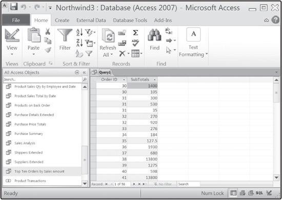
Note the presence of the SubTotals column name in Figure 9.7. The SubTotals field does not exist in the Order Details table. Rather, the SubTotals field is created in the SQL statement using the AS clause to assign a name to an expression. Although parentheses are not required, I use them in my computed field’s expression to provide readability and order of operations, if necessary.
Built-In Functions
Just as VBA incorporates many intrinsic functions such as Val, Str, UCase, and Len, SQL provides many built-in functions for determining information on your result sets. I will now show you how to use the following SQL aggregate functions:
• AVG
• COUNT
• FIRST, LAST
• MIN, MAX
• SUM
• DISTINCT
The AVG function takes an expression such as a column name for a parameter and returns the mean value in a column or other expression.
SELECT     AVG([List Price])
FROM       Products;
The preceding SQL statement returns a single value, which is the mean value of the List Price column in the Products table. Output is seen in Figure 9.8.
Notice in Figure 9.8 that the column heading gives no clue as to the meaning of the SQL statement’s return value. To correct this, simply use the AS clause as demonstrated next.
SELECT  AVG([List Price]) AS [Average Unit Price]
FROM    Products;
The COUNT function is a very useful function for determining how many records are returned by a query. For example, the following SQL query uses the COUNT function to determine how many customer records are in the Customers table.
SELECT  COUNT(*) AS [Number of Customers]
FROM    Customers;
Figure 9.9 reveals the output from the COUNT function in the preceding SQL statement. Note that it’s possible to supply a column name in the COUNT function, but the wildcard character (*) performs a faster calculation on the number of records found in a table.
FIGURE 9.8 Using the AVG function to calculate the mean value of a column.

FIGURE 9.9 Displaying the result of a COUNT function.

The FIRST and LAST functions return the first and last records in a result set, respectively. Because records are not necessarily stored in alphanumeric order, the FIRST and LAST functions may produce seemingly unexpected results. Nevertheless, the results are accurate. These functions report the first and last expressions in a result set as stored in a database and returned by the SQL query.
SELECT  FIRST([Last Name]) AS [First Employee Last Name],
        LAST([Last Name]) AS [Last Employee Last Name]
FROM    Employees;
The preceding SQL statement uses the FIRST and LAST functions to retrieve the first and last results on the last name of employee records in the Employees table. Output is seen in Figure 9.10.
FIGURE 9.10 Using the FIRST and LAST functions to retrieve the first and last values of a result set.

To determine the minimum and maximum values of an expression in SQL, use the MIN and MAX functions, respectively. Like other SQL functions, the MIN and MAX functions take an expression and return a value. The next SQL statement uses these two functions to determine the minimum and maximum unit prices found in the Products table. Output is seen in Figure 9.11.
SELECT  MIN([List Price]) AS [Minimum List Price],
        MAX([List Price]) AS [Maximum List Price]
FROM    Products;
FIGURE 9.11 Retrieving the minimum and maximum values using the MIN and MAX functions.

The SUM function takes an expression as argument and returns the sum of values. The SUM function is used in the next SQL statement, which takes a computed field as an argument to derive the sum of subtotals in the Order Details table.
SELECT  SUM([Unit Price] * Quantity) AS [Sum of Sub Totals]
FROM    [Order Details];
Output from the SQL statement using the SUM function is displayed in Figure 9.12.
The last built-in function for this section is DISTINCT, which returns a distinct set of values for an expression. For example, if I want to find a unique list of countries for the suppliers in the Northwind database, I need to sift through every record in the Suppliers table and count each unique (distinct) country name. Or, I could use the DISTINCT function to return a unique value for each country in the Country/Region column.
SELECT  DISTINCT([Country/Region])
FROM    Suppliers;
FIGURE 9.12 Displaying the output of the SUM function.

Sorting
You may recall from the discussions surrounding the FIRST and LAST functions that data stored in a database are not stored in any relevant order, including alphanumeric. Most often, data is stored in the order in which it was entered, but not always. If you need to retrieve data in a sorted manner, use the ORDER BY clause.
The ORDER BY clause is used at the end of a SQL statement to sort a result set (records returned by a SQL query) in alphanumeric order. Sort order for the ORDER BY clause can either be ascending (A to Z, 0 to 9) or descending (Z to A, 9 to 0). Use the keyword ASC for ascending or DESC for descending. Note that neither the ASC nor DESC keywords are required with the ORDER BY clause, and that the default sort order is ascending.
To properly use the ORDER BY clause, simply follow the clause with a sort key, which is a fancy way of saying a column name to sort on. The optional keywords ASC and DESC follow the sort key.
To exhibit SQL sorting techniques, study the next two SQL statements and their outputs, shown in Figures 9.13 and 9.14 respectively.
SELECT    *
FROM      Products
ORDER BY  [Product Name] ASC;
FIGURE 9.13 Using the ORDER BY clause and the ASC keyword to sort product records by product name in ascending order.

SELECT    *
FROM      Products
ORDER BY  [Product Name] DESC;
FIGURE 9.14 Using the ORDER BY clause and the DESC keyword to sort product records by product name in descending order.

Grouping
Grouping in SQL provides developers with an opportunity to group like data together. Without the use of grouping, built-in functions such as SUM and AVG would calculate every value in a column. To put like data into logical groups of information, SQL provides the GROUP BY clause.
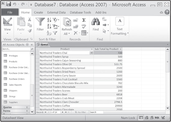
In the next SQL statement, I use the GROUP BY clause to group a computed field by product ID in the Products table.
SELECT    [Product ID], SUM([Unit Price] * Quantity) AS [Sub Total by Product]
FROM      [Order Details]
GROUP BY  [Product ID];
Notice the output from the preceding SQL statement in Figure 9.15. Even though I specified Product ID as the desired column, the output column and the data it contains show as a product name. This occurs because the Order Details table uses a SQL lookup to retrieve the Product Name by Product ID.
FIGURE 9.15 Using the GROUP BY clause to group like data together.
There are times when you need conditions on your groups. In these events, you cannot use the WHERE clause. Instead, SQL provides the HAVING clause for condition building when working with groups. To demonstrate, I modify the previous SQL statement to use a HAVING clause, which asks the database to retrieve only groups that have a subtotal by product greater than 15,000.00.
SELECT     [Product ID], SUM([Unit Price] * Quantity) AS [Sub Total by Product]
FROM       [Order Details]
GROUP BY   [Product ID]
HAVING SUM   ([Unit Price] * Quantity) > 15000.00;
Joins
Joins are used when you need to retrieve data from more than one table. Specifically, a SQL join uses keys to combine records from two tables where a primary key from one table is matched up with a foreign key from another table. The result is a combination of result sets from both tables where a match is found. If a match is not found, information from either table is discarded in the final result set.
SQL joins are created by selecting columns from more than one table in the SELECT clause, including both table names in the FROM clause, and matching like columns from both tables in the WHERE clause. The following example join’s output is shown in Figure 9.16.
SELECT   [First Name], [Last Name], [Order Date], [Ship Name]
FROM     Employees, Orders
WHERE    Employees.ID = Orders.[Employee ID];
FIGURE 9.16 Joining the Employees and Orders tables with the WHERE clause.

In Figure 9.16, I’ve retrieved columns from both the Employees and Orders tables where the Employee ID values from both tables match (ID from Employees table, and Employee ID from the Orders table). If the join keys from both tables are spelled the same I must explicitly tell SQL what table name I’m referring to by using dot notation, as seen here.
WHERE TableName.Key = TableName.Key;
Even in cases where the dot notation is not required, you can leverage the dot notation in a SELECT clause to explicitly denote which table a column belongs to, which ultimately provides readability in your queries. An example of using the dot notation in the SELECT clause for readability is seen next.
SELECT  Employees.[First Name], Employees.[Last Name], Orders.[Order Date],
        Orders.[Ship Name]
FROM    Employees, Orders
WHERE   ID = [Employee ID];
If the expression in the WHERE clause is incorrect, a Cartesian join results. A Cartesian result is when the query returns every possible number of combinations from each table involved.
The preceding join is typically called a natural join, where a row from one table matches a row from another table using a common column and matching column value. There are times however, when you want rows from one table that do not match rows in the other table. SQL solves this dilemma with an outer join.
There are two types of outer joins: left outer joins and right outer joins. A left outer join includes all records from the left (first) of the two tables even if there are no matching rows from the right (second) table. The right outer join includes all rows from the right (second) table even if there are no matching rows from the left (first) table. Outer joins are created using the LEFT JOIN or RIGHT JOIN keywords in the FROM clause, and replacing the WHERE clause with an ON clause.
To demonstrate, let’s start off with a natural join query that will show me all orders with matching invoice data.
SELECT  Orders.[Order ID], Orders.[Customer ID], Orders.[Order Date],
        Orders.[Shipped Date], Invoices.[Invoice ID], Invoices.[Invoice Date]
FROM    Orders, Invoices
WHERE   Orders.[Order ID] = Invoices.[Order ID]
There’s only one problem with this join—it’s possible I have orders that don’t yet have a matching invoice. The natural join in this case does not show me orders without an invoice. I can however, view both orders with invoices, and orders without invoices using a left outer join. You can see how to accomplish this in the following code, and the results in Figure 9.17.
SELECT  Orders.[Order ID], Orders.[Customer ID], Orders.[Order Date],
        Orders.[Shipped Date], Invoices.[Invoice ID], Invoices.[Invoice Date]
FROM    Orders LEFT JOIN Invoices
ON      Orders.[Order ID] = Invoices.[Order ID]
FIGURE 9.17 Using a left outer join to find orders with and without a matching invoice.

Looking at Figure 9.17, you can see there are orders with no matching invoice, which a natural join would have missed.
To create my outer join, I inserted the LEFT JOIN keywords into my FROM clause and replaced the WHERE keyword with the ON keyword.
FROM   Orders LEFT JOIN Invoices
ON     Orders.[Order ID] = Invoices.[Order ID]
INSERT INTO Statement
You can use SQL to insert rows into a table with the INSERT INTO statement. The INSERT INTO statement inserts new records into a table using the VALUES clause.
INSERT INTO   Books
VALUES        (‘1234abc456edf’, ‘Beginning SQL’, ‘Vine’,
              ‘Michael’, ‘Thomson Course Technology’);
Though not required, matching column names can be used in the INSERT INTO statement to clarify the fields with which you’re working.
INSERT INTO   Books (ISBN, Title, [Last Name], [First Name], Publisher)
VALUES        (‘1234abc456edf’, ‘Beginning SQL’, ‘Vine’,
              ‘Michael’, ‘Thomson Course Technology ’);
Using matching column names is necessary, not just helpful, when you only need to insert data for a limited number of columns in a table. A case in point is when working with the AutoNumber field type, which Access automatically creates for you when inserting a record.
The concept of working with an AutoNumber, and an INSERT INTO statement is shown in the following SQL statement.
INSERT INTO   Shippers (Company, [Business Phone])
VALUES        (‘Slow Boat Express’, ‘123-456-9999’);
When inserting (appending) a record into a table with the INSERT INTO statement, Access prompts you to confirm, or reverse the changes, as seen in Figure 9.18.
FIGURE 9.18 Choosing to append one row with the INSERT INTO statement.

UPDATE Statement
You can use the UPDATE statement to change field values in one or more tables. The UPDATE statement works in conjunction with the SET keyword:
UPDATE   Products
SET      [Reorder Level] = [Reorder Level] + 5;
You supply the table name to the UPDATE statement and use the SET keyword to update any number of fields that belong to the table in the UPDATE statement. In the previous UPDATE example, I updated every record’s Reorder Level field by adding the number 5. Notice that I said every record! Because I didn’t use a WHERE clause, the UPDATE statement updates every row in the table.
In the next UPDATE statement, I use a WHERE clause to put a condition on the number of rows that receive updates.
UPDATE   Products
SET      [Reorder Level] = [Reorder Level] + 5
WHERE    ID = 34;
It is possible for SQL programmers to forget to place conditions on their UPDATE statements. Because there is no undo or rollback feature after an update has successfully occurred, pay attention to the dialog box, which you see in Figure 9.19, that appears before you commit (save) changes.
FIGURE 9.19 Choosing to update one record in the Products table with the UPDATE statement.

DELETE Statement
The DELETE statement removes one or more rows from a table. It’s possible to delete all rows from a table using the DELETE statement and a wildcard as demonstrated next.
DELETE  *
FROM    Products;
More often than not, conditions are placed on DELETE statements using the WHERE clause.
DELETE  *
FROM    Products
WHERE   ID = 34;
Once again, pay close attention to Access’s informational dialog boxes when performing any inserts, updates, or deletes on tables.
The DELETE statement can perform cascade deletes on tables with one-to-many relationships if the Cascade Delete Related Records option is chosen in the Edit Relationships window, as seen in Figure 9.20.
FIGURE 9.20 Selecting cascade deletes on one-to-many table relationships.
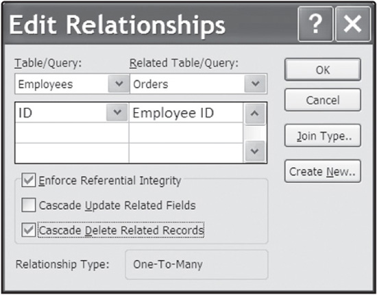
With the Cascade Delete Related Records option chosen for the Employees and Orders tables, any employee records deleted will also initiate a corresponding deletion in the Orders table where a matching Employee ID was found.
DATA DEFINITION LANGUAGE
Data definition language, also known as DDL, contains commands that define a database’s attributes. Most commonly, DDL creates, alters, and drops tables, indexes, constraints, views, users, and permissions.
In this section you investigate a few of the more common uses for DDL in beginning database programming:
• Creating tables
• Altering tables
• DROP statements
Creating Tables
Creating tables in DDL involves using the CREATE TABLE statement. With the CREATE TABLE statement, you can define and create a table, its columns, column data types, and any constraints that might be needed on one or more columns. In its simplest form, the CREATE TABLE syntax and format is shown here.
CREATE TABLE   TableName
               (FieldName FieldType,
               FieldName FieldType,
               FieldName FieldType);
The TableName attribute defines the table to be created. Each FieldName attribute defines the column to be created. Each FieldName has a corresponding FieldType attribute, which defines the column’s data type.
The next CREATE TABLE statement creates a new table called Books that contains seven columns.
CREATE TABLE   Books
               (ISBN Text,
               Title Text,
               AuthorLastName Text,
               AuthorFirstName Text,
               Publisher Text,
               Price Currency,
               PublishDate Date);
The CREATE TABLE statement allows you to specify if one or more columns should not allow NULL values. By default, columns created in the CREATE TABLE statement allow NULL entries. To specify a not NULL column, use the Not Null keywords.
CREATE TABLE   Books
               (ISBN Text Not Null,
               Title Text,
               AuthorLastName Text,
               AuthorFirstName Text,
               Publisher Text,
               Price Currency,
               PublishDate Date);
Using the Not Null keywords sets the column’s Required attribute to Yes.
Altering Tables
You can use the ALTER TABLE statement to alter tables that have already been created. Three common uses of the ALTER TABLE statement are to add column(s) to an existing table, to change the data type of one or more columns, or to remove a column from a table.
The next ALTER TABLE statement adds a Salary column to the Employees table with the help of the ADD COLUMN keywords.
ALTER TABLE   Employees
ADD COLUMN    Salary Currency;
Adding the Salary column with the ALTER TABLE statement appends the new column to the end of the Employees table. To change a column’s data type, use the ALTER COLUMN keywords in conjunction with the ALTER TABLE statement.
ALTER TABLE   Books
ALTER COLUMN  Title Memo;
In the preceding ALTER TABLE statement, I changed the data type of the Title column from a Text data type to a Memo data type.
To remove a column from a table in Access, use the DROP COLUMN keywords in conjunction with the ALTER TABLE statement:
ALTER TABLE   Employees
DROP COLUMN   Salary;
Access does not always warn you of your impending database alterations. In the case of dropping (removing) a column, Access simply performs the operation without mention.
DROP Statement
The DROP statement can be used to remove many entities from a database such as tables, indexes, procedures, and views. In this section you see how the DROP statement is used to drop a table from a database.
Removing a table from a database with the DROP statement is really quite easy. Simply supply the entity type to be dropped, along with the entity name.
DROP TABLE Books;
In the preceding example, the dropped entity typed is a TABLE and the entity name is Books. Once again, beware: Access does not always warn you when it modifies the database. In the DROP TABLE example, Access simply executes the command without any confirmation.
SUMMARY
• Most relational databases, including Access 2010, contain a version of SQL for retrieving data and manipulating database entities.
• Data definition language (DDL) is a set of SQL commands used to define attributes, such as tables and columns, of a relational database.
• Data manipulation language (DML) is a set of commands for querying, computing, sorting, grouping, joining, inserting, updating, and deleting data in a relational database.
• SQL statements are freeform, meaning one SQL statement can be written on one or more lines. For readability, SQL programmers break SQL statements into one or more logical groups on multiple lines.
• Information is retrieved from a relational database using SELECT statements.
• Simple and compound conditions can be used in SQL statements using the WHERE clause.
• Computed field values are derived using calculations in SQL statements.
• Computed fields are given display names using the AS clause.
• SQL contains many aggregate, or built-in, functions such as COUNT, DISTINCT, MIN, MAX, and SUM.
• Database records returned by a SQL statement are not sorted by default. To sort SQL query results, use the ORDER BY clause.
• SQL query results can be grouped using the GROUP BY clause.
• Natural joins are created by matching key fields in two or more tables in the WHERE clause.
• Incorrect joins can produce an unwanted Cartesian product.
• A left outer join includes all records from the left (first) of the two tables even if there are no matching rows from the right (second) table.
• A right outer join includes all rows from the right (second) table even if there are no matching rows from the left (first) table.
• Records can be manually inserted into a table using the INSERT INTO statement.
• The UPDATE statement can be used to update fields in a database table.
• Records in a table can be removed using the DELETE statement.
• Tables can be manually created using the CREATE TABLE statement.
• In its simplest form, the CREATE TABLE statement defines the table’s name, its columns, and its column types.
• The ALTER TABLE statement can be used to add columns to an existing table, update a column’s data type, and remove a column from a table.
• The DROP statement is used for removing tables, indexes, views, and procedures from a database.
Leverage the Microsoft Access 2010 Northwind database and a SQL View window for all the following challenges.
1. Write and test a SQL query that retrieves all columns from the Employee Privileges table.
2. Write and test a SQL query that retrieves only the first and last names and a business phone number from the Customers table.
3. Write and test a SQL query that uses a computed field to calculate the total cost of each record in the Order Details table.
4. Write and test the SQL query that returns the total number of records in the Employees table.
5. Use the Orders table to write and test the SQL query that returns the sum of shipping fees grouped by customer.
6. Using the INSERT INTO statement, write a SQL query that inserts a new record into the Employees table.
7. Update the unit price by $3.25 in the Products table for all products by Supplier A.
8. Delete all records in the Products table for the soups category only.
9. Using DDL commands, create a new table called HomesForSale. The HomesForSale table should contain the following fields: StreetAddress, City, State, ZipCode, SalePrice, and ListDate. Ensure that the StreetAddress column does not allow Null values.
10. Using DDL commands, add three new columns to the HomesForSale table: AgentLastName, AgentFirstName, and AgentPhoneNumber.
11. Using DDL commands, remove the HomesForSale table from the database.