| 20 | Combining Calculus with Other Tools |
In this chapter, you’ll learn how calculus can be used along with other techniques to analyze functions, optimize areas and volumes, and evaluate the properties of curves that are sometimes called conic sections because they represent cross sections of extended double cones. These curves are the circle, the ellipse, the parabola, and the hyperbola.
LOCAL MAXIMUM AND MINIMUM
Derivatives can be used to find “peaks” and “valleys,” technically called local maxima and local minima, of a function that appears as a curve when graphed. When the derivative dy/dx of a curve is equal to 0 at a certain point, the value of the function is momentarily constant. If elsewhere it varies, the value identified by dy/dx= 0 is either a local maximum or a local minimum in the function itself, as long as the second derivative, d2y/dx2, is different from 0.
If dy/dx= 0 at a point but decreases on either side, then d2y/dx2< 0 and you have a local maximum at that point, as shown in Fig. 20-1A. If dy/dx= 0 at a point but increases on either side, then d2y/dx2> 0 and you have a local minimum at that point, as shown in Fig. 20-1B. (In a few moments, you’ll see what happens if the first and second derivatives are both equal to 0 at a point.)

Figure 20-1
Examples of a local maximum (A) and a local minimum (B) in the graph of a function. Near a local maximum, the derivative decreases. Near a local minimum, the derivative increases.
As an example of how you can find local maxima and minima by means of derivatives, consider the following function:
You can tabulate some values of x and the corresponding values of y and then mark them out on graph paper. Figure 20-2A lists nine value sets that you can obtain in this way. For some curves, nine points would be enough to draw a good representation of the curve. In this case, you can get the general idea of what the curve will look like by plotting nine points, but to get a high degree of precision (not necessary for this exercise) you’d have to use a lot more.

Figure 20-2
Some tabulated points for the function y= x4 − x3 − 18x2 + 27x. At B, the points from the table are plotted on graph paper. At C, after finding the two local minima and the single local maximum by differentiation, the curve is filled in.
On the graph in Fig. 20-2B, the nine points are marked. Although they give an idea where the curve goes, they are not precise enough to let you be absolutely sure what the curve looks like. A greater number of points might help, but no matter how many points you track in a problem like this, the difficult spots are the local maximum and minimum points. Where, exactly, are they? Apparently, a local minimum exists at or near x = −3, a local maximum exists at or near x = 1, and another local minimum exists at or near x = 3. How can you find out precisely where these points are without spending all day tabulating values and making marks on graph paper, and without using a computer to zero in on these points by “brute force”?
Start out by finding the first derivative of y= x4 − x3 − 18x2 + 27x. That’s easy. You get this:
This is a cubic equation in x, so it can have 3 real number roots. Try x + 3 as a factor to represent the root at or near x = − 3. Then the cubic equation factors to
Factoring the second polynomial, a quadratic, you get (x− 3) and (4x− 3). So the whole cubic factors into
On the basis of these factors, the roots of this cubic equation are easily seen to be x = −3, x = 3, and x = 3/4. Now you know that the two minima are precisely at x = −3 and x = 3, and the maximum is at x = 3/4. From this information, you can trace out the curve on the graph paper quite accurately, as shown in Fig. 20-2C.
POINT OF INFLECTION
Here is a curve-plotting problem in which the second derivative becomes especially significant. Suppose you want to analyze the curve represented by this equation:
In Fig. 20-3A, six points are tabulated at equal, whole-number increments from x = −3 to x = 2. You can get an idea of what the graph looks like by plotting these points as shown in Fig. 20-3B. When you first glance at this set of points, you might think there is a mistake in the region between x = 0 and x = 2. Did you plot enough points? It doesn’t look like a curve in that region; it looks more like a straight line. What’s going on in this region?
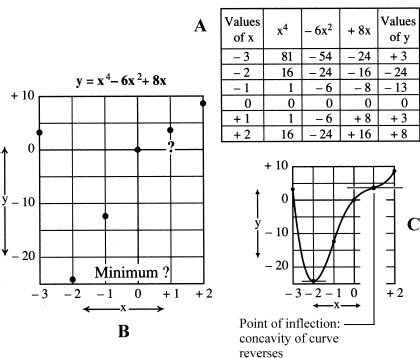
Figure 20-3
Some tabulated points for the function y= x4 − 6x2 − 8x. At B, the points from the table are plotted on graph paper. At C, after finding the first and second derivatives, the curve is filled in.
You can tabulate points at smaller intervals and then plot them, but there’s another way to find out what’s really happening to the graph of the curve in the interval between x = 0 and x = 2. The derivative of the original function is
This can be factored to
There are two roots for x = 1. What does that mean? Is it possible that there is a local maximum and a local minimum at x = 1? No, that would be a contradiction! Maybe it’s a new characteristic of curves that you haven’t seen before. Take the second derivative of the original function:
When you plug in x = 1 to this equation, you get
In a situation like this, you have neither a maximum nor a minimum, but something else, called an inflection point, or a point of inflection. When the second derivative of a function is equal to 0 at a particular point, it means that the concavity of the function reverses at that point. That can happen in either of two ways: the curve can change from concave downward to concave upward as the value of the independent variable increases, or it can go the other way, changing from concave upward to concave downward. If you fill in the graph by connecting the points (Fig. 20-3C), you can see that in this case, the inflection point at x = 1 is a place where the curve goes from concave downward to concave upward as you make the value of x more positive.
If you aren’t sure what concavity means, look again at Fig. 20-1. The curve in the top part of drawing A is concave downward, and the curve in the top part of drawing B is concave upward. Some mathematicians prefer to use the term “convexity” instead of “concavity.” If a curve is concave downward, then it’s convex upward; if it’s concave upward, then it’s convex downward. Think of concave and convex mirrors!
In the example of Fig. 20-3C, the slope of the function happens to be 0 at the inflection point. That means the curve is momentarily horizontal. This is often the case at inflection points, but not always. It is possible for a curve to have an inflection point where the slope, and therefore the first derivative, is not equal to 0. The graph of the function y= tan x is a good example. When x = 0, the curve is at an inflection point going from concave downward to concave upward; but the slope, represented by dy/dx, is equal to 1. To see how this works, use your calculator to locate points and plot a precision graph of y = tan x for a couple of dozen values between, say, x = −π/4 and x = π/4.
MAXIMUM AND MINIMUM SLOPE
Now, let’s return the function considered earlier in this chapter under the heading “Local maximum and minimum”:
The second derivative of this is
Equating this to 0 and making it into a quadratic equation produce roots of x = −1.5 and x = 2. The second derivative is equal to 0 where a graph of the first derivative reaches a local maximum or a local minimum. A local maximum in the first derivative is a point of maximum slope (steepest upward) in the original function. Similarly, a local minimum in the first derivative is a point of minimum slope (steepest downward) in the original function. This information can help you plot graphs even more accurately, as shown in Fig. 20-4 for the function y = x4 − x3 − 18x2 + 27x.

Figure 20-4
At A, a closer analysis of the graph of y= x4 − x3 − 18x2 − 27x, along with its first and second derivatives. At B, some points of significance in this curve.
MAXIMUM AREA WITH CONSTANT PERIMETER
One practical use of differentiation is to find the shape of a rectangle that produces the maximum possible interior area for a given perimeter. You can derive the formula for the area of a rectangle with constant perimeter, as shown in Fig. 20-5. Let p represent one-half of the perimeter of the rectangle. Let x represent the length of one side, and let p − x represent the length of the adjacent side. Then the area A is

Figure 20-5
Differentiation can be used to find the shape of a rectangle with the largest interior area for a constant perimeter. We determine the maximum for the quadratic as shown.
The derivative of the area with respect to x is
Setting dA/dx = 0, you can solve the resulting equation and get 2x = p or x = (1/2)p. This tells you that the area is maximum when the rectangle is a square with equal dimensions both ways.
If the area of the rectangle is kept constant, the perimeter varies, and the minimum perimeter is solved for, the result is the same. If you like, work it out that way as an “extra credit” exercise!
BOX WITH MINIMUM SURFACE AREA
Now you’ve seen that a square represents the best shape for a rectangle, assuming you want to get the smallest possible perimeter for a given constant area, or the most area for a given constant perimeter. (Did you already suspect that? Now you’ve mathematically proved it!) Here’s a similar problem. How tall should a square-based box of constant volume be, if you want to have the minimum possible surface area?
Assume that the constant volume of the box is V, and the length of each edge of the base is x, as shown in Fig. 20-6A. The volume is x3, so the height must be V/x2. You have a top and bottom that each have an area of x2, and four sides that each have an area of x times V/x2, which reduces to V/x. Therefore, the total surface area A is
Differentiating with respect to x while holding V constant gives you this:
If you set this equal to 0 with the idea that you’ll get a minimum, you have
You want this to be 0 for all possible values of x! That happens if and only if V = x3, making the height equal to the length of the edges of the square base. It follows that the box must be a cube. You’re not surprised by this result, are you?
To make this exercise more interesting, suppose that the box has a square base but no top, as shown in Fig. 20-6B. Now, the total surface area of the box is 4V/x + x2. Differentiating gives

Figure 20-6
Differentiation can be used to figure out the shape of a box for minimum surface area when the volume is constant. At A, the box has a closed top; at B, the box has an open top.
This is equal to 0 if and only if V = x3/2, making the height equal to one-half the length of the edges of the square base.
CYLINDER WITH MINIMUM SURFACE AREA
Here is another optimization problem that differentiation can solve. Suppose you have a right circular cylinder, and you want to minimize its surface area for a constant volume. (A right circular cylinder has an axis perpendicular to its base, and a base that is a perfect circle. It is the object that most people imagine when they think of a cylinder.)
The volume V of a right circular cylinder of radius r and height h is
The surface area of the top, which is a disk, is πr2; the same is true for the bottom. For the curved surface, the area is 2πrh. So the total surface area A of a cylinder such as the one shown in Fig. 20-7A, including the top and the bottom, is

To obtain only one variable, write h in terms of the constant V and the variable r, so you obtain this:
By substituting and rearranging, the equation for total area becomes
The derivative of the area A with respect to the radius r is
The value of this function is 0 when V = 2πr3. To find h, substitute this in the original formula for V at the beginning of this section, getting
This solves to h = 2r. Twice the radius is the diameter, so you can say that the minimum surface area exists when the height of the cylinder equals its diameter.
Suppose you want a cylindrical container with no top, as shown in Fig. 20-7B. Following the same method as you did for the open box, you will determine that the height needs to be equal to the radius, which is one-half the diameter.

Figure 20-7
Differentiation can be used to figure out the shape of a right circular cylinder for minimum surface area when the volume is constant. At A, the cylinder has a closed top; at B, the cylinder has an open top.
CONE WITH MINIMUM SURFACE AREA
What is the best shape for an ice cream cone? You want one in which the cone will hold a given volume with minimum surface area.
The volume V of a right circular cone (one in which the axis is perpendicular to the circular top, as shown in Fig. 20-8) is

Figure 20-8
Differentiation can be used to figure out the shape of a right circular cone, not including the disk-shaped top, for minimum surface area when the volume is constant.
The surface area A, not including the circular top, is
where l is the slant height of the cone, measured from a point on the edge of the circular top down to the apex. If you want to write it in terms of h instead, you get
Substituting to get h in terms of V and r, then substituting that into the second equation for A, differentiating and equating to zero, you find that h, for minimum surface area, is equal to the square root of 2 multiplied by r. That means the height should be approximately 1.414 times the radius, or 0.707 times the diameter. You can follow along with the calculations in Fig. 20-8 to see how it works.
This problem, looked at in a different way, is one of finding the most volume for a given constant surface area. Do you see many ice cream cones that are wider at the top than they are tall? No? If they were the optimum shape, maybe ice cream vendors would make less profit per cone, but their customers would be happier.
EQUATIONS FOR CIRCLES, ELLIPSES, AND PARABOLAS
Figure 20-9 illustrates three common second-order curves: the circle, the ellipse, and the parabola. They are called second-order because they can all be expressed by equations that go no higher than the second power (or square) of the independent variable. At A, C, and E in the figure, you will see the equation, in its simplest form, for each of these curves. In using these equations, both the circle and the ellipse are centered at the origin, where x = 0 and y = 0. The parabola is different. It rests on the origin, but extends upward in the positive y direction for negative or positive values of x. Note that the parabola is symmetric with respect to the y axis. This property is called bilateral symmetry.
In drawings B, D, and F in Fig. 20-9, you will see more general equations for the same curves, which are not necessarily centered or resting on the origin. Instead, the point on which the curve is centered or rests is at x = a and y = b. Deriving these general forms is a simple matter. You merely substitute (x − a) for x and (y − b) for y in the original simple form, and then multiply out. Notice that the relationship between the second-order terms (those that involve x2 and y2) is not affected by this transformation. This fact lets you recognize curves that are circles, ellipses, or parabolas from their respective equations.

Figure 20-9
Second-order curves. At A, circle centered at the origin. At B, general circle. At C, ellipse centered at the origin. At D, general ellipse. At E, parabola “resting” on the origin. At F, general parabola. In drawings B, D, and F, the origin is indicated by the letter o.
In the circle, r represents the radius. In the ellipse, two constants replace the radius, designated q and s. These constants represent one-half the principal axes of the ellipse. These principal axes can be regarded as maximum (major) and minimum (minor) diameters of the ellipse. In the case of the parabola, the curve is symmetrical on either side of a vertical line x = a, and rests on the horizontal line defined by y = b. The constant f in Fig. 20-9E and F determines the “sharpness” of the curve. If f is positive, the parabola opens upward. If f is negative, the curve opens downward.
DIRECTRIX, FOCUS, AND ECCENTRICITY
When you examine Fig. 20-9, you can see that the parabola is fundamentally different from the circle and the ellipse. The circle and ellipse are closed; the parabola is open. A circle can be drawn with an instrument called a compass that has its point at the center. An ellipse can be drawn with a device that uses two centers to elongate it. But how can you generate a parabola?
If you drive around a circular racetrack, you do not have a compass attaching you to the center of the track! You must direct your course with the steering wheel. Paralleling that idea, visualize going along a parabolic course, positioning yourself with respect to two things, a focus and a directrix. The focus is a point, and the directrix is a straight line, as shown in Fig. 20-10. If you want to follow a parabola, you must stay equidistant (equally far away) from the focus and the directrix at all times. That constant distance is designated u. Now imagine a straight line passing through the focus and intersecting the directrix at a right angle. Along this line, the two equal distances are each called the focal length and are symbolized f. Drawing a line through the focus parallel to the directrix, you can divide u, measuring your distance from the directrix, into 2f and y.

Figure 20-10
All the points on a the curve of a parabola are equidistant from the focus and the directrix.
In Fig. 20-10, Fact 1 relates to the u that expresses your distance from the focus. Fact 2 relates to the u that expresses your distance from the directrix. Combine these equations, rearrange the result, and you have an equation of the same form as the equation for the parabola in Fig. 20-9F. Because the two distances denoted by u are equal, this curve has an eccentricity of 1, or unity.
THE ELLIPSE AND THE CIRCLE
Now suppose you have a curve in which the eccentricity e is less than 1 but larger than 0. You can use the same geometric arrangement to determine the eccentricity as you did with the parabola, but now the distance from the focus is eu instead of u, as shown in the two examples of Fig. 20-11. When the value of e is between, but not including, 0 and 1, mathematicians write it this way:

Figure 20-11
At A, construction of an ellipse based on a defined focus and directrix. At B, an ellipse with smaller eccentricity is more nearly a circle. When the eccentricity becomes equal to 0, the ellipse becomes a circle.
Apply the same two facts and combine them, as you did for the parabola. You will end up with an equation for an ellipse.
As the eccentricity e approaches 0, the center of the ellipse gets farther from the directrix, eu gets closer to f in value, and the ellipse gets less elongated. If you set e = 0, the equation simplifies so that it represents a circle, and then f = r. Going the other way, as the eccentricity e approaches 1, the center of the ellipse gets closer to the directrix, the value of eu gets farther from f, and the ellipse gets more elongated. If the eccentricity e reaches 1, the ellipse “breaks open” at one end and becomes a parabola. Now you know three things about second-order curves:
• If e = 0, you have a circle.
• If 0 < e < 1, you have an ellipse.
• If e = 1, you have a parabola.
What happens if e becomes greater than 1? You’ll find out soon!
RELATIONSHIPS BETWEEN FOCUS, DIRECTRIX, AND ECCENTRICITY
Look at these three curves—the circle, the ellipse, and the parabola—in terms of the new parameters. The circle has a single focus, which is the center, and the directrix removes itself to infinity. (You can imagine it as infinitely far away in any direction. Or, if you prefer, you can consider it not to exist at all.) Viewed as an algebraic equation for a circle, the coefficients of the second-order terms, x2 and y2, are equal.
The ellipse has two foci at finite distance from each other. The ellipse is bilaterally symmetric with respect to a straight line connecting these foci. As is the case with the circle, the algebraic equation of the ellipse has two second-order terms, x2 and y2, but their coefficients are not equal. With two symmetric foci, the ellipse has two directrixes at finite distances.
The parabola can be viewed as having two foci: one finite and one infinite. Its single directrix is at a distance equal to the focal length. Its algebraic equation has only one second-order term.
The properties of these three second-order curves are summarized in Fig. 20-12.

Figure 20-12
Basic characteristics of circles, ellipses, and parabolas.
FOCUS PROPERTY OF PARABOLA
You can rearrange the equation for a parabola to get an equation for x in terms of y and the focal length f. Looking at Fig. 20-13, examine the angles at a specific point (x, y) on the curve: θ is the angle between a line from the focus and the parabola’s axis, and φ is the slope of the curve expressed as an angle relative to the x axis. Then you can see that the following trigonometric properties hold true:
and

Figure 20-13
The focal property of a parabola defines how a reflector of this shape can focus or direct visible light, sound, or radio waves.
Using these facts and by examining the drawing and calculations in Fig. 20-13, you can deduce the relationship θ= 2φ. This is significant, because it defines the way a parabolic reflector can focus or direct beams of radiant energy.
When a ray emerges from the focal point, it always travels in a straight line. Eventually, unless it runs right along the axis of the parabola, the ray strikes the parabola and is reflected from it. Remember from physics that the angle of incidence equals the angle of reflection. If you analyze the drawing in Fig. 20-13 carefully, you will see that any ray emerging from the focus reflects from the parabola parallel to the axis. This is how a lantern, searchlight, or radar transmitting antenna works. In the reverse sense, any ray coming in parallel to the axis will strike the parabola and be reflected to the focal point. This is how a reflecting telescope or dish-type radio receiving antenna works.
FOCUS PROPERTY OF ELLIPSE
Applying the same idea to an ellipse, you can write equations based on the axes, as shown in Fig. 20-14. In this example, a is one-half the length of the major axis, and b is one-half the length of the minor axis. These are called the major semiaxis and the minor semiaxis, respectively. The eccentricity is e. Just follow along with the calculations in the drawing. You will discover that the following two equations hold true:
and

Figure 20-14
Relationships between the eccentricity of an ellipse and the lengths of the major and minor semi-axes.
The angular relationship of the parabola explains why a light source at the focus reflects into a parallel outgoing beam, and why a parallel incoming beam converges on the focus. Extending this to the ellipse, instead of focusing into a parallel beam (Fig. 20-15A), the curve focuses rays from one focal point to the other (Fig. 20-15B).

Figure 20-15
Reflection properties of a parabola (at A) and an ellipse (at B).
Have you ever been in a room where the walls were curved, intersecting the floor in a huge ellipse? You can stand at one focus and have a friend stand at the other. When your friend whispers, it sounds as if he is speaking right into both of your ears at the same time. It works even better in a special room with a three-dimensional, egglike shape called an ellipsoid, which results from the rotation of an ellipse around its major axis. A suspended walkway runs along the major axis. When two people stand so their heads are exactly at the foci, they can whisper to each other even if the ellipse is many feet across. Rooms like this have actually been built to demonstrate the principle!
HYPERBOLA: ECCENTRICITY GREATER THAN 1
The circle has eccentricity equal to 0; the ellipse has eccentricity larger than 0 but less than 1; the parabola has an eccentricity of exactly 1. What happens if the eccentricity is greater than 1? You get a curve called a hyperbola.
Look at the equations for each type of curve. For the circle, the coefficients of x2 and y2 are equal. For the ellipse, they are unequal. For the parabola, one is of the coefficients is equal to 0. In the case of the hyperbola, one of the coefficients reverses its sign. That is, one of them is negative and the other is positive.
Let’s compare equations for a generalized circle, a generalized ellipse, and a generalized hyperbola, each centered at the origin. For the circle, you have
where r is the radius. For the ellipse, you have
where q and s are the lengths of the semiaxes. For the hyperbola, you have
where q and s are again called the semiaxes, but in a different sense from the ellipse.
Figure 20-16 shows an example of a hyperbola. (The ellipse between the curves is there for reference only; it defines the semiaxes q and s.) The hyperbola appears, upon casual inspection, like two parabolas back to back. But there’s an important difference in the shape of a hyperbola compared with the shape of a parabola. The parameters that help define hyperbolas are straight lines called asymptotes. In Fig. 20-16, there are two asymptotes through the origin (the point where x = 0 and y = 0) whose equations are
and

Figure 20-16
Fundamental properties of a hyperbola. The central ellipse is drawn for reference only; it is not part of the hyperbola itself.
The curve approaches the asymptotes as you move away from the origin. However, the curve never quite touches the asymptotes, no matter how far from the origin you go.
Parabolas do not have asymptotes. Hyperbolas always have them. If the asymptotes intersect at right angles to each other, the major and minor semiaxes have equal length. Then q = s, and the curve is called a right hyperbola.
In the simplest cases, such as the one shown in Fig. 20-16, the asymptotes of a hyperbola intersect at the origin. However, they can intersect at any point x = a and y = b. Then the equation of the hyperbola generalizes to this:
This is the counterpart of the generalized equation for the ellipse from Fig. 20-9D:
where x = a and y = b represent the point where the axes (instead of the asymptotes) intersect. If q = s, then the ellipse is a circle.
GEOMETRY OF CONIC SECTIONS
At the beginning of this chapter, you were introduced to the notion of a conic section. What, you ask, do cones have to do with circles, ellipses, parabolas, and hyperbolas? The answer can be found in the ways flat planes and double cones intersect.
Imagine a double right circular cone that extends infinitely both upward and downward, as shown in the drawings of Fig. 20-17. Now imagine a flat, infinitely large plane that can be moved around so it slices through the cone in various ways. The intersection between the plane and the double cone will always be a circle, an ellipse, a parabola, or a hyperbola.

Figure 20-17
The conic section scan be defined by the intersection of a flat plane with a double cone. At A, a circle. At B, an ellipse. At C, a parabola. At D, a hyperbola.
Figure 20-17A shows what happens when the plane is perpendicular to the axis of the double cone. In that case, you get a circle. In Fig. 20-17B, the plane is not perpendicular to the axis of the cone, but it isn’t tilted very much. The curve is still closed, but it isn’t a circle; it’s an ellipse. As the plane tilts farther away from a right angle with respect to the double-cone axis, the ellipse becomes more elongated; its eccentricity increases. Then you reach an angle of tilt where the curve is no longer closed. At this threshold, the intersection between the plane and the cone is a parabola (Fig. 20-17C), and the eccentricity is equal to 1.
So far, the plane has only intersected one-half of the double cone. If you keep tilting the plane beyond the angle at which the intersection is a parabola, the plane will intersect both halves of the cone. Then you get a hyperbola, and the eccentricity is greater than 1. The greatest possible tilt, where the plane is parallel to the axis of the double cone, produces a hyperbola with the maximum possible eccentricity, as shown in the example of Fig. 20-17D.
QUESTIONS AND PROBLEMS
This is an open-book quiz. You may refer to the text in this chapter (and earlier ones, too, if you want) when figuring out the answers. Take your time! Consider all values given as exact, so you don’t have to worry about significant figures. The correct answers are in the back of the book.
1. Find the point (x, y) at which the graph of the following function attains its maximum value:
2. Consider the following function:
There are infinitely many points (x, y) at which the slope of this function is maximum. Write a general expression for these points.
3. Suppose you are standing on a large, frozen lake at night, holding a flashlight. The beam from the flashlight is cone-shaped. The outer face of the light cone subtends a 20˚ angle with respect to the axis (the ray corresponding to the beam center). How can you aim the flashlight to form a circular region of light on the ice?
4. In the situation described in Prob. 3, how can you point the flashlight so the edge of the region of light forms an ellipse on the ice?
5. In the situation described in Prob. 3, how can you aim the flashlight so the edge of the region of light forms a parabola on the ice?
6. In the situation described in Prob. 3, how can you aim the flashlight so the edge of the region of light forms a half-hyperbola on the ice?
7. Determine x and y intercepts, local maxima, local minima, and inflection points (if any) for these functions. Specify the points as ordered pairs (x, y), where y = f(x).
(a) f(x) = 2x3 − 5
(b) f(x) = (x2 + 3)(x− 4)
(c) f(x) = 2 tan x
(d) f(x) = 3 cos x
8. Using the information you obtained in solving Prob. 7, plot graphs of the functions given. Intercept points, local maxima, local minima, and points of inflection (if any) should be labeled. Otherwise, the curves can be approximately drawn.
..................Content has been hidden....................
You can't read the all page of ebook, please click here login for view all page.